Coupled dynamic analysis of horizontal axis floating offshore wind turbines with a spar buoy floater

Abstract

Coupled dynamic analysis of a floating offshore wind turbine (FOWT) is predicted with in-house ITU-WAVE computational tool. The hydrodynamic parameters are approximated with time marching of boundary integral equation whilst aerodynamic parameters are solved with unsteady blade element momentum method. In addition, forces on FOWT due to mooring lines are predicted with quasi-static analysis whilst hydrodynamic viscous effects are included with Morison equation. FOWT’s blades are considered as an elastic structure whilst tower is considered as a rigid structure. The effects of steady wind speed on surge motion spectrum decrease the spectrum amplitude over wave frequency ranges, but this effect is not significant. The duration of time domain simulation plays significant role in the region of surge and pitch resonant frequencies. The numerical results of in-house ITU-WAVE computational code for eigenfrequencies of blades, aerodynamics and hydrodynamics parameters are validated against other numerical results which shows satisfactory agreements.

Introduction

The issue of global warming has resulted in growing pressure on governments in the world to exploit the renewable sources for power generation to reduce the carbon dioxide emissions. Of these, wind energy is globally distinguished as a leading technology for non-polluting energy generation. As the wind energy industry has grown considerably, electricity generated by wind power has shown a dramatic fall in cost (www.windeurope.org). As the offshore environment has higher capacity factor than onshore due to steadier and stronger wind velocity, Floating Offshore Wind Turbines (FOWT) in deep-water offshore environments has emerged as a forward-thinking application of this technology for utilising unexploited large potential offshore wind resources for the large-scale generation of electricity. However, despite current progress, wind power still has some way to go before it fulfils its potential as a large-scale supplier of electricity.

The design of FOWT requires the dynamic coupling of the aerodynamic, hydrodynamic, mooring and structural dynamics as a whole energy system. Of these integrated dynamic coupling, the aerodynamic loads are the function of the relative wind velocity over aerofoils of blades. The relative wind velocity consists of the effects of undisturbed wind velocity at hub height, induced velocity due to rotation of the wake and motion of FOWT (e.g. blade rotation, local blade velocity due to the elastic deformation of the blade if the blades are not considered as a stiff structure, translational and rotational velocity of floater). The unsteady aerodynamic forces in time domain due to interaction between wind and wind turbine blades are modelled using different methods including simple empirical approximation assuming known thrust coefficients (Utsunomiya et al., 2013), strips (unsteady Blade Element Momentum (BEM) method), panel methods, vortex methods or full Navier-Stokes approximations. The unsteady BEM method couple the momentum theory with two-dimensional strip theory (Glauret, 1935) to predict the aerodynamic loads at each strip. The unsteady BEM method is very fast and gives accurate prediction, and currently is used in many developed codes (FAST, SIMO-RIFLEX, HAWC2, ITU-WAVE). The three-dimensional effects to consider the details of the flow characteristics around wind turbine blades are considered in inviscid vortex (Milne-Thomson, 1966) and panel (Hess, 1975) aerodynamic methods. The restrictions over viscous effects are achieved using viscous Computational Fluid Dynamics (CFD) methods (Make and Vaz, 2015). However, the viscous CFD models will require a large effort for input preparation and post processing compared to unsteady BEM or panel methods and are also very expensive computationally which are not suited for routine applications today.

The two and three-dimensional numerical methods are used to predict the hydrodynamic parameters due to the interaction of floating systems with incident waves. The two-dimensional strip theory methods (Salvensen et al., 1970) are used successfully in academia and industry due to accurate prediction of hydrodynamic parameters compared to experimental methods. The strip theory methods consider the flow around the floating system two dimensional and ignore the interactions between strips. In addition, strip theory methods do not predict the low frequency region accurately which are predicted with unified theory methods (Breit and Sclavounos, 1986; Kashiwagi, 1993). As the two-dimensional methods do not consider interactions between strips, the three-dimensional methods using panels to describe surfaces of floating systems are used to overcome the shortcoming of the two-dimensional methods taking interaction effects between discretised panels into account automatically. Although three-dimensional viscous CFD methods could be used for accurate prediction of hydrodynamic parameters, they are computationally intensive and expensive for practical use. The computational time could be significantly reduced using inviscid CFD methods known as three-dimensional panel methods which are suited better for practical use and predict the hydrodynamic parameters accurately compared to experimental results (Kara, 2021a, 2021b, 2022a). Of the panel methods, Rankine Panel methods (Kring and Sclavounos, 1991; Nakos and Sclavounos, 1990; Xiang and Faltinsen, 2011) and wave Green function methods (Kara, 2000; King, 1987; Liapis, 1986) are widely used in academia and industry due to their accurate predictions of the design parameters. Rankine Panel methods require the discretion of both body surface and free surface to satisfy the body boundary condition, free surface boundary condition and condition at infinity whilst wave Green function methods require only discretisation of body surface to satisfy body boundary condition as the free surface boundary condition and condition at infinity is satisfied automatically by Green function. The potential methods do not include the effects of viscosity which can be considered through computationally inexpensive Morison equation (Nielsen et al., 2006) together with three-dimensional potential methods. If the characteristic dimensions (e.g. length) of the floaters are small compared to wavelength, the wave loads due to viscosity effects are an important wave loads for design purpose and needs to be considered. In addition, viscosity effects play significant role in the case of the flow separation.

Mooring lines as a station-keeping system is used to keep FOWT in position so that FOWT can perform its intended functions safely. As there are no hydrostatic stiffness due to motion of FOWT in surge, sway and yaw modes, mooring line stiffnesses are used to predict the natural frequencies at these modes. The accurate predictions of the mooring line stiffnesses are also particularly important as they would directly affect the time simulation of FOWT. Mooring stiffnesses, the tension forces induced by mooring lines and moments exerted by tension forces can be predicted either quasi-static or full dynamic analysis (Al-Solihat and Nahon, 2016; Hall et al., 2014). The quasi-static analysis, which is computationally very efficient, predicts stiffnesses, forces and moments analytically in static equilibrium. The quasi-static analysis assumes that the waves are linear, and platform and mooring line velocities are also small. The fully dynamic analyses are required if the dynamic effects of hydrodynamic drag, mooring line inertia and added mass due to disturbance of mooring lines, which are neglected in quasi-static analysis, are considerably important for the prediction of stiffness, forces and moments.

The floating systems including FOWT could be considered as rigid or elastic structures depending on how the motion of the floating systems effects the pressure field around them. If the weakly coupling exists, the floating systems are considered as rigid structures where the contribution of rigid body motion much higher than that of elastic motion to the pressure field around FOWT. In this case, the analyses of structures, hydrodynamics and aerodynamics are independent from each other and performed separately. However, in the case of fully coupled analyses, elastic behaviour of floating system needs to be considered under aeroelasticity and hydroelasticity. The aerodynamic and structural analyses where structure above mean sea level are strongly coupled in aeroelasticity whilst hydrodynamic and structural analyses where structure below mean sea level are considerably coupled in hydroelasticity. It is also considered that the eigenfrequencies due to elastic motion are much higher than the range of the frequencies due to wind and wave loads in the case of weakly coupled analysis (Hansen et al., 2006; Kagemoto and Yue, 1993; Kara, 2015, 2021c; Ohkusu, 1974; Wolgamot et al., 2012). In addition, the stiffness of the structures is much greater compared to restoring coefficients due to wave loading in the case of hydrodynamic analysis and weakly coupling. The greater eigenfrequencies and structural stiffnesses imply that the contribution of elastic motion to aerodynamic and hydrodynamic loadings is negligible in weakly coupled analysis. The fatigue life and steady state global elastic vibration of the floating systems could be significantly affected due to fully coupling of the structural, aerodynamic and hydrodynamic analyses where the eigenfrequencies of the elastic deflections of the floating structures are at the same range with the frequencies due to aerodynamic and hydrodynamic loadings (Hansen et al., 2006; Kara, 2015, 2021b, 2021c).

In the present paper, National Renewable Energy Laboratory (NREL) offshore 5 MW baseline wind turbine with spar-buoy platform is used to predict the wind power prediction directly in time domain. The dynamic analysis couples the aerodynamic, aeroelasticity, hydrodynamics and mooring analyses in time domain. The aerodynamic loads due to wind environment are predicted using unsteady BEM method whilst the aeroelastic behaviour of the wind turbine blades are considered as Euler-Bernoulli cantilever beam. Mooring stiffness and forces on platform due to mooring lines are approximated using the quasi-static analysis. Impulse Response Functions (IRFs) of hydrodynamic radiation and diffraction forces (e.g. diffraction and Froude-Krylov) are predicted using the transient wave Green function (Kara, 2010, 2011, 2016b, 2020b, 2022a). The time marching of boundary integral equation is used to obtained IRFs which are then used for the time simulation of the coupled equation of motion to approximate the acceleration, velocity and displacement of the coupled floating system. The present numerical results of in-house ITU-WAVE for aero-hydro-elastic coupled floating system are compared with experimental and other numerical results (Jonkman and Musail, 2010) for validation purpose.

Equation of motion of FOWT

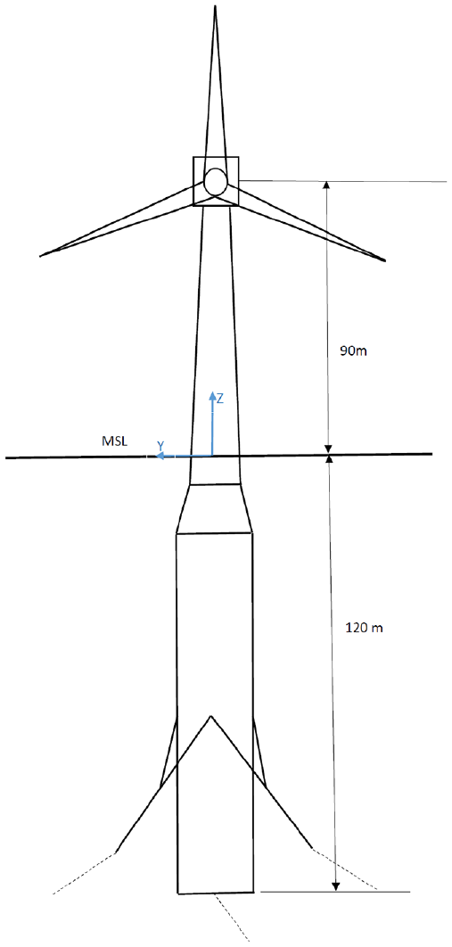
Figure 1 shows the horizontal axis FOWT and the body-fixed coordinate system to describe the fluid behaviour around FOWT and used to predict the aerodynamic and hydrodynamic loads. The coordinate system, $\overrightarrow{x}=(x,y,z)$ , is a right-handed and fixed to the platform (or floater) on Mean See Level (MSL). The centre of the xy-plane on z = 0 is selected as the origin of the coordinate system on the free surface in which forward, transverse and upward directions represent x-direction, y-direction and z-direction respectively. The interaction of wind and incident wave with FOWT in Figure 1 cause the floating system to oscillate in its mean position.

Figure 1.

Horizontal axis FOWT with a spar buoy platform/floater.

The dynamic behaviour of FOWT in equation (1), which couples aerodynamic, hydrodynamic and mooring analyses, is presented with time domain equation of motion (Cummins, 1962). The motion of FOWT is caused by applied external forces including first order diffraction forces, forces due to mooring lines, aerodynamic forces and viscous forces. The motion of FOWT due to external forces are balanced with the inertia of FOWT, hydrostatic restoring forces, hydrodynamic wave damping and stiffness of mooring lines. The oscillations of FOWT in mean position generates waves that exist until the motion decays to zero. This behaviour is represented with convolution integral in the left-hand-side of equation (1). The oscillations due to external forces also affect the pressure field around FOWT causing forces and moments on floating system all subsequent times.

$$\sum _{k=1}^6(M_{\mathrm{jk}}+a_{\mathrm{jk}}){\stackrel{··}{x}}_k\left(t\right)+b_{\mathrm{jk}}{\stackrel{·}{x}}_k\left(t\right)+(C_{\mathrm{jk}}^M+C_{\mathrm{jk}}+c_{\mathrm{jk}})x_k\left(t\right)+{\int }_0^{t}d\tau K_{\mathrm{jk}}^R(t-\tau ){\stackrel{·}{x}}_k(\tau )=F_j^E(t)$$

(1)

where rigid-body translational modes of surge, sway and heave are given with $j=1,2,3$ respectively whilst rotational modes of roll, pitch and yaw are presented with $j=4,5,6$ respectively. The displacement of FOWT is given with $x_k(t)$ whilst ${\stackrel{·}{x}}_k\left(t\right)$ and ${\stackrel{··}{x}}_k\left(t\right)$ where dots represent the time derivatives with respect to displacement $x_k(t)$ are used for velocity and acceleration respectively. The mass of floater, tower, nacelle and rotor blades are presented with inertia $M_{\mathrm{jk}}$ matrix. The restoring coefficients matrices due to motion of FOWT and mooring lines are presented with $C_{\mathrm{jk}}$ and $C_{\mathrm{jk}}^M$ respectively. The instantaneous responses of FOWT to fluid motion are given with $c_{\mathrm{jk}}$ , $b_{\mathrm{jk}}$ and $a_{\mathrm{jk}}$ in equation (1) which are frequency and time independent matrices, and corresponding to displacement related restoring forces, velocity related wave damping and acceleration related added mass at infinity respectively. The time dependent forces are predicted using impulsive velocity such that $K_{\mathrm{jk}}^R(t)$ accounting free surface effect of the fluid response due to oscillations of FOWT is the radiation IRF and represents the forces in $j^{\mathrm{th}}$ direction due to an impulsive velocity in $k^{\mathrm{th}}$ direction on FOWT. $K_{\mathrm{jk}}^R(t)$ is the function geometry of floater and time (Ogilvie, 1964). $F_j^E(t)$ in equation (1) is the total exciting forces and moments in time domain and given as

$$F_j^E\left(t\right)={\int }_{-\infty }^{\infty }d\tau K_j^D(t-\tau )\zeta (\tau )+\sum _{i=1}^{N_M}{F}_{\mathrm{ji}}^M(t)+F_j^A\left(t\right)+F_j^V\left(t\right)$$

(2)

The kernel $K_j^D\left(t\right)$ in equation (2) are the diffraction IRFs. The impulsive wave elevation with a uni-direction and heading angle $\beta$ (King, 1987) results in diffraction IRFs $K_j^D\left(t\right)$ which is the superposition of scattering and Froude-Krylov IRFs. The diffraction force predicted using an arbitrary wave elevation at the origin of body-fixed coordinate system in Figure 1 is obtained due to the incident wave elevation $\zeta (t)$ . $F_{\mathrm{ji}}^M(t)$ is the total forces and moments due to mooring lines whilst $N_M$ ( $i=1,2,3,\dots ,N_M$ ) is the total number of mooring lines. $F_{\mathrm{ji}}^M(t)$ is predicted using quasi-static analysis (Al-Solihat and Nahon, 2016). $F_j^A\left(t\right)$ is the aerodynamic forces and moments and predicted by unsteady BEM method (Hansen, 2008) whilst $F_j^V\left(t\right)$ represents the viscous drag effects and predicted by Morison equation (Morison et al., 1950). Once the inertia matrix, stiffness matrix, radiation forces due to wave and total external excitation forces in equation (2) due to wave, wind, mooring and viscosity are known, the coupled dynamic equation of motion of FOWT in equation (1) may be simulated with fourth order Runge-Kutta method (Kara, 2016a, 2016c, 2017, 2018, 2020a).

Aerodynamic analysis

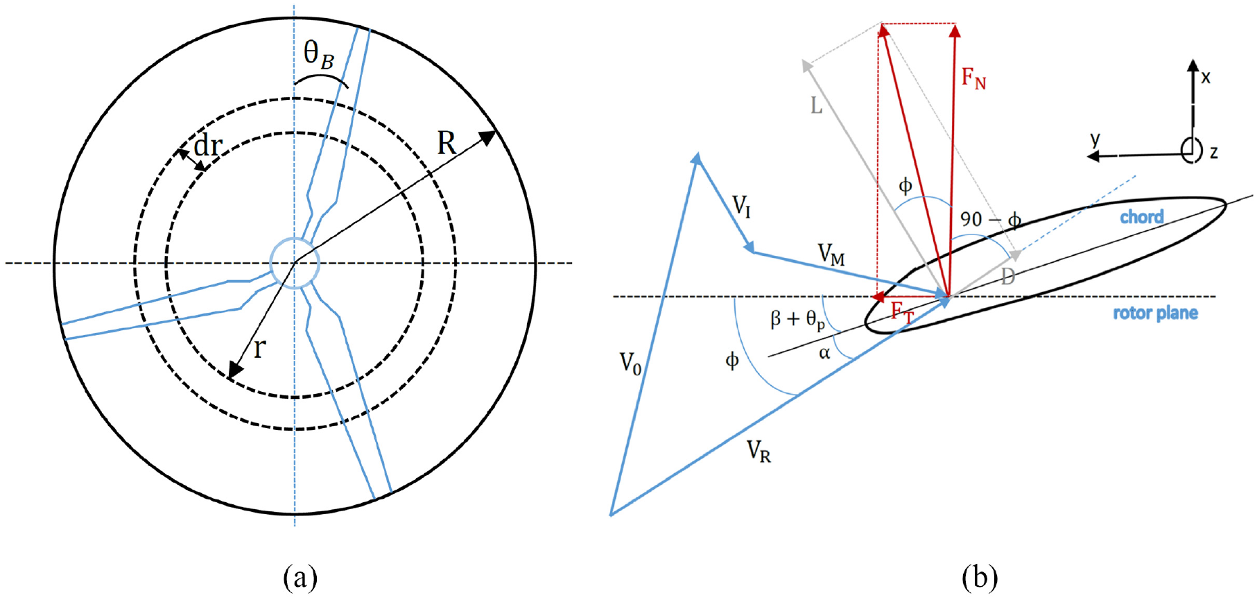
The aerodynamic parameters are predicted with two-dimensional aerofoils in Figure 2(b) in which it is assumed that velocity components are calculated in the xy-plane and velocity in z-direction is considered zero. It is also assumed that flow around the aerofoils is two-dimensional considering the velocity in streamwise are much greater than spanwise velocity. In the context of two-dimensional analysis, unsteady BEM model (Glauert, 1935) is used to predict the time series of the loads for time-varying input, pitch angle, thrust force, torque moment, power and steady loads in a range of rotational speed and wind speeds. The momentum theory is coupled with blade element model in unsteady BEM to calculate aerodynamic variables including the twist and chord distribution.

Figure 2.

(a) Annular model and (b) wind velocity components seen locally and forces acting on an aerofoil.

Aerodynamic loads on two-dimensional aerofoils

The relative wind velocity ${\mathbf{V}}_{\mathrm{R}}$ in equation (3) on an aerofoil, which is a strip of a blade in Figure 2(b), consists of the undisturbed wind velocity ${\mathbf{V}}_0$ , the induced velocity ${\mathbf{V}}_{\mathrm{I}}$ and the motion velocity ${\mathbf{V}}_{\mathrm{M}}$ ( ${\mathbf{V}}_{\mathrm{M}}={\mathbf{V}}_{\mathrm{rot}}+{\mathbf{V}}_{\mathrm{B}}+{\mathbf{V}}_{\mathrm{P}})$ . The motion velocity ${\mathbf{V}}_{\mathrm{M}}$ consists of the rotational velocity ${\mathbf{V}}_{\mathrm{rot}}$ , platform velocity ${\mathbf{V}}_{\mathrm{P}}$ and local blade velocity ${\mathbf{V}}_{\mathrm{B}}$ which consider the aeroelastic behaviour of the blade where the blade is not considered a stiff structure (Hansen, 2008).

$${\mathbf{V}}_{\mathrm{R}}={\mathbf{V}}_0+{\mathbf{V}}_{\mathrm{I}}-{\mathbf{V}}_{\mathrm{rot}}-{\mathbf{V}}_{\mathrm{B}}-{\mathbf{V}}_{\mathrm{P}}$$

(3)

Once the relative wind velocity ${\mathbf{V}}_{\mathrm{R}}$ in equation (3), which is of important to accurately predict as it affects the prediction of all other aerodynamic parameters, is calculated with unsteady BEM method, it can be used for the determination of relative wind angle in equation (4) which is the angle between the relative wind velocity and rotor plane in Figure 2(b).

$$\tan \varphi =\frac{{\mathrm{V}}_{\mathrm{R}}^{\mathrm{x}}}{-{\mathrm{V}}_{\mathrm{R}}^{\mathrm{y}}}$$

(4)

where ${\mathrm{V}}_{\mathrm{R}}^{\mathrm{x}}$ and ${\mathrm{V}}_{\mathrm{R}}^{\mathrm{y}}$ are the x- and y-components of relative wind velocity ${\mathbf{V}}_{\mathrm{R}}$ respectively. The relative wind angle $\varphi$ in equation (4) is then used to predict another important parameter of the local angle of attack $\alpha$ in equation (5) which requires accurate prediction and is the angle between relative wind velocity and cord line of the aerofoil in Figure 2(b). The chord line is the straight line which connect the trailing edge and leading edge of aerofoil.

$$\alpha =\varphi -\mathrm{\theta },\mathrm{\alpha }=\varphi -(\beta +{\theta }_{\mathrm{p}})$$

(5)

The local pitch angle of the blade in equation (5) is given with $\theta ={\theta }_{\mathrm{p}}+\beta$ which is the angle between rotor plane and chord line in Figure 2(b). The local pitch angle $\theta$ consists of the twist of the blade $\beta$ and pitch angle ${\theta }_{\mathrm{p}}$ . The angle between the rotor plane and tip chord is the pitch angle ${\theta }_{\mathrm{p}}$ whilst the twist $\beta$ is measured relative to the tip chord. Once the angle of attack $\alpha$ is determined, the experimentally available lift ${\mathrm{C}}_{\mathrm{l}}$ and drag ${\mathrm{C}}_{\mathrm{d}}$ coefficients are then predicted as a function of the angle of attack $\alpha$ . The known lift ${\mathrm{C}}_{\mathrm{l}}$ and drag ${\mathrm{C}}_{\mathrm{d}}$ coefficients are then used to calculate the lift force $\mathrm{L}$ and the drag force $\mathrm{D}$ per unit length in equations (6) and (7) respectively.

$$\mathrm{L}=\frac{1}{2}{\rho \mathrm{V}}_{\mathrm{R}}^2\mathrm{c}{\mathrm{C}}_{\mathrm{l}}$$

(6)

$$\mathrm{D}=\frac{1}{2}{\rho \mathrm{V}}_{\mathrm{R}}^2\mathrm{c}{\mathrm{C}}_{\mathrm{d}}$$

(7)

where $\rho$ is the air density whilst $\mathrm{c}$ is the chord length. The normal force ${\mathrm{F}}_{\mathrm{N}}$ and tangential force ${\mathrm{F}}_{\mathrm{T}}$ per unit length, which are required for the calculation of thrust force and torque, are then predicted in equations (8) and (9) respectively.

$${\mathrm{F}}_{\mathrm{N}}=\mathrm{Lcos}\varphi +\mathrm{Dsin}\varphi$$

(8)

$${\mathrm{F}}_{\mathrm{T}}=\mathrm{Lsin}\varphi -\mathrm{Dcos}\varphi$$

(9)

The rotor is turned with shaft torque which is delivered with the tangential load component ${\mathrm{F}}_{\mathrm{T}}$ in equation (9). In addition, a solidity $\sigma (\mathrm{r})$ in equation (10) is the fraction of the annular area covered by blades in the control volume in Figure 2(a).

$$\sigma \left(\mathrm{r}\right)=\frac{\mathrm{Bc}(\mathrm{r})}{2\pi \mathrm{r}}$$

(10)

where $\mathrm{r}$ is the radial position of the control volume, $\mathrm{c}(\mathrm{r})$ is the local chord and $\mathrm{B}$ denotes the number of blades. The normal force ${\mathrm{F}}_{\mathrm{N}}$ and tangential force ${\mathrm{F}}_{\mathrm{T}}$ per unit length are then used to predict the thrust force $\mathrm{dT}$ in equation (11), torque $\mathrm{dM}$ in equation (12) and mechanical power $\mathrm{dP}$ in equation (13) on the control volume of thickness $\mathrm{dr}$ in Figure 2(a).

$$\mathrm{dT}=\mathrm{B}{\mathrm{F}}_{\mathrm{N}}\mathrm{dr}$$

(11)

$$\mathrm{dM}=\mathrm{rB}{\mathrm{F}}_{\mathrm{T}}\mathrm{dr}$$

(12)

$$\mathrm{dP}=\omega \mathrm{dM}$$

(13)

where rotor’s angular velocity is given with $\omega$ . The discontinuity of the pressure drops over rotor is provided with a disc which is considered as a rotor. The pressure drops result in the thrust force $\mathrm{dT}$ in streamwise direction which causes the windspeed to be reduced from upstream to downstream. The wake of the rotor is deflected due to a normal velocity ${\mathrm{V}}_{\mathrm{I}}^{\mathrm{n}}(={\mathrm{V}}_{\mathrm{I}}^{\mathrm{x}})$ in the rotor plane which results from the pressure drop causing the thrust force $\mathrm{dT}$ . Assuming only the lift force results in induced velocity ${\mathrm{V}}_{\mathrm{I}}$ which is in the opposite direction to the lift force in Figure 2(b). The normal induced velocity ${\mathrm{V}}_{\mathrm{I}}^{\mathrm{n}}$ in x-direction (Bramwell, 1976) is given in equation (14).

$${\mathrm{V}}_{\mathrm{I}}^{\mathrm{n}}(={\mathrm{V}}_{\mathrm{I}}^{\mathrm{x}})=\frac{\mathrm{BLcos}\varphi }{4\pi \rho \mathrm{rF}|{\mathbf{V}}_0+{\mathrm{f}}_{\mathrm{g}}\mathbf{n}(\mathbf{n}·{\mathbf{V}}_{\mathrm{I}}|}$$

(14)

and tangential components ${\mathrm{V}}_{\mathrm{I}}^{\mathrm{t}}(={\mathrm{V}}_{\mathrm{I}}^{\mathrm{y}})$ of induced velocity ${\mathbf{V}}_{\mathrm{I}}$ is given in equation (15)

$${\mathrm{V}}_{\mathrm{I}}^{\mathrm{t}}(={\mathrm{V}}_{\mathrm{I}}^{\mathrm{y}})=\frac{\mathrm{BLsin}\varphi }{4\pi \rho \mathrm{rF}|{\mathbf{V}}_0+{\mathrm{f}}_{\mathrm{g}}\mathbf{n}(\mathbf{n}·{\mathbf{V}}_{\mathrm{I}})|}$$

(15)

where the unit vector $\mathbf{n}=(-1,0,0)$ represents a vector in the thrust force $\mathrm{dT}$ direction. Assuming that there are no interactions between annular elements, in other words, elements are free from radial dependency. In the case of infinite number of blades with a rotor, the acting forces on each annular element are constant. The shortcoming of infinite number of blades are overcame with Prandtl’s tip loss factor $\mathrm{F}$ in equations (14) and (15) (Glauert, 1935) and is presented in equation (16) which result in a rotor to be considered with a finite number of blades. The vortex behaviour in the wake of a rotor with a finite number of blades is different compared to a rotor with an infinite number of blades.

$$\mathrm{F}=\frac{2}{\pi }\mathrm{co}{\mathrm{s}}^{-1}\left({\mathrm{e}}^{-\frac{\mathrm{B}(\mathrm{R}-\mathrm{r})}{2\mathrm{rsin}\varphi }}\right)$$

(16)

where the rotor’s radius is given with $\mathrm{R}$ presented in Figure 2(a). When the axial induction factor, $\mathrm{a}$ , becomes larger than approximately $\mathrm{a}=0.4$ , the simple momentum theory breaks down. The fractional decrease of upstream velocity on the surface of blade is presented with the axial induction factor, $\mathrm{a}$ . Glauert correction factor ${\mathrm{f}}_{\mathrm{g}}$ in equations (14) and (15) (Glauert, 1935) for high values of axial induction factor, $\mathrm{a}$ , is introduced to overcome this shortcoming. Glauert correction factor ${\mathrm{f}}_{\mathrm{g}}$ in equations (14) and (15) in the turbulent wake state and is given in equation (17).

$${\mathrm{f}}_{\mathrm{g}}=\{\begin{array}{c}1\mathrm{for}\mathrm{a}\le {\mathrm{a}}_{\mathrm{c}}\hfill \\ \multicolumn{1}{c}{\frac{{\mathrm{a}}_{\mathrm{c}}}{\mathrm{a}}(2-\frac{{\mathrm{a}}_{\mathrm{c}}}{\mathrm{a}})\mathrm{for}\mathrm{a}>{\mathrm{a}}_{\mathrm{c}}}\end{array}$$

(17)

${\mathrm{a}}_{\mathrm{c}}$ is around 0.2 and determined with equations (18) and (19)

$$\mathrm{if}\mathrm{a}\le {\mathrm{a}}_{\mathrm{c}}\mathrm{a}=\frac{1}{1+\mathrm{K}}$$

(18)

$$\mathrm{if}\mathrm{a}>{\mathrm{a}}_{\mathrm{c}}\mathrm{a}=\frac{1}{2}[2+\mathrm{K}(1-2{\mathrm{a}}_{\mathrm{c}})-\sqrt{{(\mathrm{K}(1-2{\mathrm{a}}_{\mathrm{c}})+2)}^2+4({\mathrm{Ka}}_{\mathrm{c}}^2-1)}]$$

(19)

where $\mathrm{K}=4\mathrm{Fsi}{\mathrm{n}}^2\varphi /\sigma {\mathrm{C}}_{\mathrm{n}}$ in which normal force coefficient is given with ${\mathrm{C}}_{\mathrm{n}}={\mathrm{F}}_{\mathrm{N}}/\frac{1}{2}{\rho \mathrm{V}}_{\mathrm{R}}^2\mathrm{c}$ . Equations (18) and (19) are the functions of relative wind angle $\varphi$ , relative wind velocity ${\mathrm{V}}_{\mathrm{R}}$ and angle of attack $\alpha$ and need to be solved iteratively until the prediction approaches to a defined tolerance value. It is assumed that the time step Δt in time domain simulation is small which implicitly means that when the induced velocity ${\mathrm{V}}_{\mathrm{I}}$ components is updated for new values to predict the tangential ${\mathrm{V}}_{\mathrm{I}}^{\mathrm{t}}$ component in equation (15) and normal ${\mathrm{V}}_{\mathrm{I}}^{\mathrm{n}}$ component in equation (14), the values at previous time step can be used for convergence of the induced velocity ${\mathrm{V}}_{\mathrm{I}}$ components . As the induced velocity ${\mathrm{V}}_{\mathrm{I}}$ changes relatively slowly in time, this is an acceptable assumption.

Dynamic inflow prediction

The unsteady performance of FOWT results in the instationary behaviour of the aerodynamic loads on blades and other parts of FOWT. The instationary effects result in the dynamic inflow and instationary profile aerodynamic. The dependence of the sectional aerodynamical forces on the time varying angle of attack $\alpha$ including the effects of the shed vorticity are accounted with the instationary profile aerodynamics. The ratio of the chord to the effective velocity seen by the blade section, $\mathrm{c}/(\omega ·\mathrm{r})$ , determines the characteristic time scale of profile aerodynamic which vary approximately 0.01 second at the tip and 0.2 second at blade for a wind turbine with diameter D of the order 50 m. On the other hand, the wake induced unsteadiness of the flow in the rotor plane is affected with the dynamic inflow. The influence of the time varying trailing wake vorticity on the inflow velocity in the rotor plane is accounted with the dynamic inflow. $\mathrm{D}/{\mathrm{V}}_0$ represents the characteristic time scale of the dynamic inflow which is in the order of 5–10 seconds. The time scale of the profile aerodynamic is one to two orders of magnitude smaller than that of the dynamic inflow which can be considered as quasi-steady phenomena having a time scale large compared to that of profile aerodynamic (Snel and Schepers, 1995).

The vectorial sum of the instantaneous free stream velocity ${\mathbf{V}}_0$ , motion velocity ${\mathbf{V}}_{\mathrm{M}}$ and the velocity induced by the wake of FOWT, ${\mathbf{V}}_{\mathrm{I}}$ , is used to predict the velocity field of rotor plane as presented in equation (3). The induced velocity ${\mathbf{V}}_{\mathrm{I}}$ is to be modelled as dynamic inflow. The trailing vorticity and shed vorticity are the part of the time dependent wake vorticity. The effect of vorticity on the angles of attack $\alpha$ in the wake determines the strength of shed and trailing vorticity. The interaction of vorticity and angles of attack can be attributed to the lifting line theory of Prandtl (van Holten, 1976). The trailing vorticity results in the dynamic inflow. The present dynamic inflow model is applied using unsteady BEM equations with contribution from a time derivative of intermediate induced velocity ${\mathbf{V}}_{\mathrm{I}}^{\mathrm{int}}$ and final induced velocity ${\mathbf{V}}_{\mathrm{I}}$ to take the time delay into account before the equilibrium of the aerodynamic loads in equations (14) and (15). Two first order differential equations in equations (20) and (21) in the present study are used to model the dynamic inflow to filter the induced velocities (Øye, 1991).

$${\mathbf{V}}_{\mathrm{I}}^{\mathrm{int}}+{\tau }_1\frac{{\mathbf{dV}}_{\mathrm{I}}^{\mathrm{int}}}{\mathrm{dt}}={\mathbf{V}}_{\mathrm{I}}^{\mathrm{qs}}+\mathrm{k}·{\tau }_1\frac{{\mathbf{dV}}_{\mathrm{I}}^{\mathrm{qs}}}{\mathrm{dt}}$$

(20)

$${\mathbf{V}}_{\mathrm{I}}+{\tau }_2\frac{\mathbf{d}{\mathbf{V}}_{\mathrm{I}}}{\mathrm{dt}}={\mathbf{V}}_{\mathrm{I}}^{\mathrm{int}}$$

(21)

where $\mathrm{k}=0.6$ is a constant, ${\mathbf{V}}_{\mathrm{I}}^{\mathrm{qs}}$ the quasi-static value found using equations (14) and (15). The intermediate induced velocity is given with ${\mathbf{V}}_{\mathrm{I}}^{\mathrm{int}}$ whilst the final filtered induced velocity is given with ${\mathbf{V}}_{\mathrm{I}}$ . A vortex method is used to calibrate the time constants ${\tau }_1$ and ${\tau }_2$ with equations (22) and (23).

$${\tau }_1=\frac{1.1}{(1.0-1.3\mathrm{a})}\frac{\mathrm{R}}{{\mathrm{V}}_0}$$

(22)

$${\tau }_2=(0.39-0.26{\left(\frac{\mathrm{r}}{\mathrm{R}}\right)}^2){\tau }_1$$

(23)

Equations (20) and (21) are solved analytically assuming that the right-hand sides are constant. The backward difference is used to predict the right-hand-side of equation (20) in equation (24) where ${\mathbf{V}}_{\mathrm{I}}^{\mathrm{q}{\mathrm{s}}^{\mathrm{i}}}$ is obtained by the solution of equations (14) and (15).

$$\mathbf{H}={\mathbf{V}}_{\mathrm{I}}^{\mathrm{q}{\mathrm{s}}^{\mathrm{i}}}+\mathrm{k}·{\tau }_1\frac{{\mathbf{V}}_{\mathrm{I}}^{\mathrm{q}{\mathrm{s}}^{\mathrm{i}}}-{\mathbf{V}}_{\mathrm{I}}^{\mathrm{q}{\mathrm{s}}^{\mathrm{i}-1}}}{\Delta \mathrm{t}}$$

(24)

The intermediate induced velocity ${\mathbf{V}}_{\mathrm{I}}^{\mathrm{in}{\mathrm{t}}^{\mathrm{i}}}$ is then obtained by solving equation (20) analytically in equation (25)

$${\mathbf{V}}_{\mathrm{I}}^{\mathrm{in}{\mathrm{t}}^{\mathrm{i}}}=\mathrm{H}+({\mathbf{V}}_{\mathrm{I}}^{\mathrm{in}{\mathrm{t}}^{\mathrm{i}-1}}-\mathrm{H}){\mathrm{e}}^{-\frac{\Delta \mathrm{t}}{{\tau }_1}}$$

(25)

The final filtered induced velocity ${\mathbf{V}}_{\mathrm{I}}^{\mathrm{i}}$ is obtained solving equation (21) analytically in equation (26),

$${\mathbf{V}}_{\mathrm{I}}^{\mathrm{i}}={\mathbf{V}}_{\mathrm{I}}^{\mathrm{in}{\mathrm{t}}^{\mathrm{i}}}+({\mathbf{V}}_{\mathrm{I}}^{\mathrm{i}-1}-{\mathbf{V}}_{\mathrm{I}}^{\mathrm{in}{\mathrm{t}}^{\mathrm{i}}}){\mathrm{e}}^{-\frac{\Delta \mathrm{t}}{{\tau }_2}}$$

(26)

Capturing the time behaviour of the power and loads requires the application of a dynamic filter for the induced velocity ${\mathbf{V}}_{\mathrm{I}}^{\mathrm{i}}$ when the thrust is changed by pitching the blades.

Dynamic stall prediction

The impulsive forces are replaced with added mass assuming incompressible flow as Mach number are lower than 0.3 for FOWT. In addition, it is also assumed that the leading-edge separation for the relative thick aerofoils having thickness of no less than 15% used on wind turbine blades is not dominant. These assumptions lead Theodorsen theory (Theodorsen, 1935) which takes lift under attached flow conditions into account, and under stalled flow conditions only trailing edge separation is considered.

The atmospheric turbulence, tower passage, yaw/tilt misalignment and wind shear result in the constant changes of the wind seen locally on a point on the blade. The angle of attack $\alpha$ changes dynamically during the revolution due to this direct impact. A time delay, which is proportional to the chord divided by the relative velocity seen at the blade section, would happen due to the effect of changing the blade’s angle of attack. The separation of flow from boundary layer whether partly separated or attached over aerofoils affects the response of the aerodynamic loads. Theodorsen theory (Theodorsen, 1935) for unsteady lift and aerodynamic moment can be used to predict the time delay in the case of attached flow. A separation function ${\mathrm{f}}_{\mathrm{s}}$ (Øye, 1991) can be used to model the dynamic stall, in the case of trailing edge stall at increasing angles of attack $\alpha$ , where the separation starts at the trailing edge and gradually increases upstream. The attached flow, compressibility effects and leading-edge separation are taken further into account with the Beddoes–Leishman model (Leishman and Beddoes, 1989) which also corrects the drag and moment coefficients. The dynamic aerofoil data is mostly affected with trailing edge separation although the linear region can also contribute (Hansen et al., 2004). It is important to notice that non-existent vibrations of flapwise can be computed if a dynamic stall model is ignored Øye (1991). The separation function ${\mathrm{f}}_{\mathrm{s}}$ describes the degree of stall for trailing edge stall in equation (27).

$${\mathrm{C}}_{\mathrm{l}}={\mathrm{f}}_{\mathrm{s}}{\mathrm{C}}_{\mathrm{l}}^{\mathrm{inv}}\left(\alpha \right)+(1-{\mathrm{f}}_{\mathrm{s}}){\mathrm{C}}_{\mathrm{l}}^{\mathrm{fs}}\left(\alpha \right)$$

(27)

where ${\mathrm{f}}_{\mathrm{s}}=1$ represents fully attached flow, ${\mathrm{f}}_{\mathrm{s}}=0$ is used for fully separated flow. The lift coefficient of inviscid flow without any separation is given with ${\mathrm{C}}_{\mathrm{l}}^{\mathrm{inv}}$ whilst that of fully separated flow is given with ${\mathrm{C}}_{\mathrm{l}}^{\mathrm{fs}}$ . The linear region of the static aerofoil is used to predict ${\mathrm{C}}_{\mathrm{l}}^{\mathrm{inv}}$ with extrapolation (Hansen et al., 2004) where ${\mathrm{C}}_{\mathrm{l}}^{\mathrm{fs}}$ and ${\mathrm{f}}_{\mathrm{s}}^{\mathrm{st}}$ are also predicted. ${\mathrm{f}}_{\mathrm{s}}^{\mathrm{st}}$ is the value of ${\mathrm{f}}_{\mathrm{s}}$ that reproduces the static aerofoil data in equation (27) assuming the static value will be always achieved with ${\mathrm{f}}_{\mathrm{s}}$ .

$$\frac{\mathrm{d}{\mathrm{f}}_{\mathrm{s}}}{\mathrm{dt}}=\frac{{\mathrm{f}}_{\mathrm{s}}^{\mathrm{st}}-{\mathrm{f}}_{\mathrm{s}}}{\tau }$$

(28)

Equation (29) is obtained by integrating equation (28) analytically:

$${\mathrm{f}}_{\mathrm{s}}(\mathrm{t}+\Delta \mathrm{t})={\mathrm{f}}_{\mathrm{s}}^{\mathrm{st}}+({\mathrm{f}}_{\mathrm{s}}\left(\mathrm{t}\right)-{\mathrm{f}}_{\mathrm{s}}^{\mathrm{st}}){\mathrm{e}}^{-\frac{\Delta \mathrm{t}}{\tau }}$$

(29)

$\tau =\mathrm{A}·\mathrm{c}/{\mathrm{V}}_{\mathrm{R}}$ is used to predict the time constant $\tau$ in equation (29) where $\mathrm{A}$ is a constant value equalling 4.0. The static value is trying to be approximated by aerofoil data with angle of attack $\alpha$ changing in time in dynamic stall model. This implies that in the case of increasing the angle of attack $\alpha$ from below to above stall, some of the inviscid (unstalled) value ${\mathrm{C}}_{\mathrm{l}}^{\mathrm{inv}}$ are contained in the unsteady aerofoil data. This also means that the development of boundary layer from one state to another needs time.

Wind loads on FOWT tower

The average wind factor ${\mathrm{C}}_{\mathrm{Tw}}$ is used to approximate the wind load ${\mathrm{F}}_{\mathrm{Tw}}$ in equation (30) on tower of FOWT (Matsukuma and Utsunomiya, 2008).

$${\mathrm{F}}_{\mathrm{Tw}}=\frac{1}{2}{\mathrm{C}}_{\mathrm{Tw}}\rho {\mathrm{V}}_0{\left(\mathrm{z}\right)}^2{\mathrm{D}}_{\mathrm{Tw}}\left(\mathrm{z}\right)$$

(30)

where the wind velocity at height $\mathrm{z}$ above mean sea level is given with ${\mathrm{V}}_0\left(\mathrm{z}\right)$ whilst the diameter of the tower at the height $\mathrm{z}$ is given with ${\mathrm{D}}_{\mathrm{Tw}}\left(\mathrm{z}\right)$ . The power law is used to predict the vertical variation of the wind velocity ${\mathrm{V}}_0\left(\mathrm{z}\right)$ in equation (31).

$${\mathrm{V}}_0\left(\mathrm{z}\right)={\mathrm{V}}_0\left(\mathrm{H}\right){\left(\frac{\mathrm{z}}{\mathrm{H}}\right)}^{\nu }$$

(31)

where the hub height between hub and mean sea level is presented with $\mathrm{H}$ whilst the height from mean sea level being $\mathrm{z}$ . The amount of velocity shear changing in the range of 0.1 and 0.25 is represented with $\nu$ (Hansen, 2008).

Dynamic structural analysis

The prediction of the deflections and velocities of FOWT’s blades in the time domain requires the structural analysis. The time dependent aerodynamic loads calculated with unsteady BEM method in sections 2.1.1–2.1.3 are then used to predict the dynamic structural response of FOWT’s blades. The structural and aerodynamic models are highly coupled and must be solved together in the case of an aeroelastic analysis. The time domain equation of motion including generalised mass matrix, ${\mathbf{M}}_{\mathrm{g}}$ , damping matrix, ${\mathbf{B}}_{\mathrm{g}}$ and stiffness matrix, ${\mathbf{K}}_{\mathrm{g}}$ for a discretised mechanical system is given in equation (32)

$${\mathbf{M}}_{\mathrm{g}}\stackrel{··}{\mathrm{x}}\left(\mathrm{t}\right)+{\mathbf{B}}_{\mathrm{g}}\stackrel{·}{\mathrm{x}}\left(\mathrm{t}\right)+{\mathbf{K}}_{\mathrm{g}}\mathrm{x}\left(\mathrm{t}\right)={\mathbf{F}}_{\mathrm{g}}\left(\mathrm{t}\right)$$

(32)

where the generalised force vector associated with the external loads are given with ${\mathbf{F}}_{\mathrm{g}}\left(\mathrm{t}\right)$ . The acceleration, velocities and displacements (deformations) are approximated assuming linear stiffness and damping in equation (32). The number of degrees of freedom is represented with the number of elements in deformations $x(t)$ . A linear combination of a few basis functions corresponding to the eigenmodes with the lowest eigenfrequencies is used to describe a deflection shape with modal shape functions describing the deflection of the rotor blades for a FOWT. The aeroelastic behaviour of the blades in the present study are presented with first three eigenmodes (e.g. two flapwise and one edgewise). It is known that the numerical results with three eigenmodes are in satisfactory agreement with measurements which indicate the validity of the assumption (Øye, 1996). The linear combination of mass ${\mathbf{M}}_{\mathrm{g}}$ and stiffness ${\mathbf{K}}_{\mathrm{g}}$ matrices using Rayleigh damping ${\mathbf{B}}_{\mathrm{g}}$ are used to predict the structural damping in equation (33).

$${\mathbf{B}}_{\mathrm{g}}={\alpha }_1{\mathbf{M}}_{\mathrm{g}}+{\alpha }_2{\mathbf{K}}_{\mathrm{g}}$$

(33)

where ${\alpha }_1=0.0$ and ${\alpha }_2=0.03$ are constants that are related to mass and stiffness matrices respectively (Cheng et al., 2017). Fourth order Runge-Kutta method (Kara, 2021a, 2021b, 2022a) is used to solve the equation of motion in time domain in equation (32).

Hydrodynamic analysis

The hydrodynamic loads on the floater of FOWT are predicted using a combination of the time dependent Morison’s equation and potential flow theory. The time and frequency independent restoring coefficients are predicted on the mean position of the platform. The inviscid effects of the hydrodynamic diffraction and radiation forces (Kara, 2021b, 2022a, 2022b, 2022c) are considered with the convolution integrals which are the part of the three-dimensional transient boundary integral equation whilst the viscous effects are taken using Morison equation into account (Morison et al., 1950).

Time domain boundary integral equation and its solutions

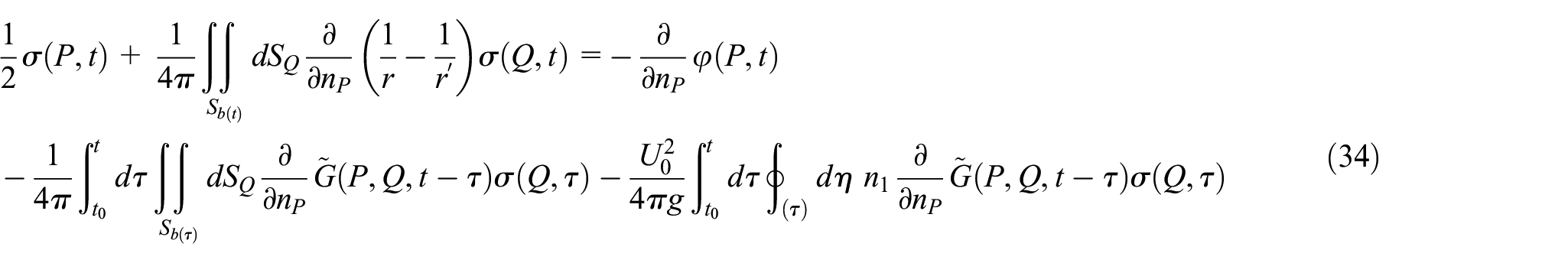
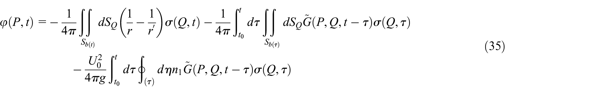
The time dependent boundary integral equation in equations (34) and (35) is used to solve the initial boundary value problem after applying potential theory and Green theorem over the time domain wave Green function. The solution of the initial boundary value problem requires to satisfy the condition at infinity, free surface boundary condition, body boundary condition and initial condition. The transient wave Green function $\tilde{\mathrm{G}}(\mathrm{P},\mathrm{Q},\mathrm{t}-\tau )$ satisfy the free surface boundary condition, condition at infinity and initial conditions automatically. This results in only body boundary condition to be satisfied numerically for the solution of the time dependent boundary integral equation (Wehausen and Laitone, 1960). The source strength $\sigma (P,t)$ is obtained by solving the boundary integral equation in equation (34) with time marching scheme (Kara, 2021b)

$$\begin{array}{c}\multicolumn{1}{c}{\frac{1}{2}\sigma (P,t)+\frac{1}{4\pi }\int \underset{S_{b\left(t\right)}}{\int }d{S}_Q\frac{\partial }{\partial n_P}(\frac{1}{r}-\frac{1}{r^{\prime }})\sigma (Q,t)=-\frac{\partial }{\partial n_P}\phi (P,t)}\\ \multicolumn{1}{c}{-\frac{1}{4\pi }{\int }_{t_0}^{t}d\tau \int \underset{S_{b\left(\tau \right)}}{\int }d{S}_Q\frac{\partial }{\partial n_P}\tilde{G}(P,Q,t-\tau )\sigma (Q,\tau )-\frac{U_0^2}{4\pi g}{\int }_{t_0}^{t}d\tau {\oint }_{\left(\tau \right)}d\eta n_1\frac{\partial }{\partial n_P}\tilde{G}(P,Q,t-\tau )\sigma (Q,\tau )}\end{array}$$

(34)

and time dependent potential $\phi (P,t)$ over floater

$$\begin{array}{c}\multicolumn{1}{c}{\phi (P,t)=-\frac{1}{4\pi }\int \underset{S_{b\left(t\right)}}{\int }d{S}_Q(\frac{1}{r}-\frac{1}{r^{\prime }})\sigma (Q,t)-\frac{1}{4\pi }{\int }_{t_0}^{t}d\tau \int \underset{S_{b\left(\tau \right)}}{\int }d{S}_Q\tilde{G}(P,Q,t-\tau )\sigma (Q,\tau )}\\ \multicolumn{1}{c}{-\frac{U_0^2}{4\pi g}{\int }_{t_0}^{t}d\tau {\oint }_{\left(\tau \right)}d\eta n_1\tilde{G}(P,Q,t-\tau )\sigma (Q,\tau )}\end{array}$$

(35)

where $(\frac{1}{\mathrm{r}}-\frac{1}{{\mathrm{r}}^{\prime }})$ is the time independent Rankine part whilst $\tilde{\mathrm{G}}(\mathrm{P},\mathrm{Q},\mathrm{t}-\tau )$ is the memory (or transient) part $\tilde{\mathrm{G}}(\mathrm{P},\mathrm{Q},\mathrm{t}-\tau )$ representing the effect of the free surface in time due to the disturbances of the floater. The diagonal and off-diagonal elements of the influence (or interaction) matrix are predicted with Rankine parts $(\frac{1}{\mathrm{r}}-\frac{1}{{\mathrm{r}}^{\prime }})$ where distances between field point $\mathrm{P}(\mathrm{x},\mathrm{y},\mathrm{z})$ and source (or integration) point $Q(\xi ,\mathrm{\eta },\mathrm{\zeta })$ are given with $\mathrm{r}=\sqrt{{(\mathrm{x}-\xi )}^2+{(\mathrm{y}-\eta )}^2+{(\mathrm{z}-\zeta )}^2}$ whilst distances between image source point and field point are given with $\mathrm{r}\prime =\sqrt{{(\mathrm{x}-\xi )}^2+{(\mathrm{y}-\eta )}^2+{(\mathrm{z}+\zeta )}^2}$ . Rankine parts $(\frac{1}{\mathrm{r}}-\frac{1}{{\mathrm{r}}^{\prime }})$ are predicted with analytical integration over each quadrilateral element (Hess and Smith, 1964). The predictions of Rankine part are calculated using the relative positions of the field and integration points for $\mathrm{r}$ whilst it is field points and image integration points for $\mathrm{r}\prime$ . In the case of large values of $\mathrm{r}$ and $\mathrm{r}\prime$ , a monopole expansion is used whilst it is a multi-pole expansion for intermediate values. In the case of small values of $\mathrm{r}$ and $\mathrm{r}\prime$ , the exact solution is used.

The free surface effect due to the interaction of the platform with incident wave, and due also to the oscillations of the platform are presented with the memory part of Green function, $\tilde{\mathrm{G}}(\mathrm{P},\mathrm{Q},\mathrm{t}-\tau )=2{\int }_0^{\infty }\mathrm{dk}\sqrt{\mathrm{kg}}\sin (\sqrt{\mathrm{kg}}(\mathrm{t}-\tau )){\mathrm{e}}^{\mathrm{k}(\mathrm{z}+\zeta )}{\mathrm{J}}_0(\mathrm{kR})$ where $\mathrm{g}$ is the gravitational acceleration whilst the wave number is given with $\mathrm{k}$ . The zero order Bessel function is presented with ${\mathrm{J}}_0(\mathrm{kR})$ whilst the distances on the free surface between source points $Q(\xi ,\mathrm{\eta },\mathrm{\zeta })$ and field points $\mathrm{P}(\mathrm{x},\mathrm{y},\mathrm{z})$ are given with $R=\sqrt{{(\mathrm{x}-\xi )}^2+{(\mathrm{y}-\eta )}^2}$ . The memory part of Green function $\tilde{\mathrm{G}}(\mathrm{P},\mathrm{Q},\mathrm{t}-\tau )$ is first analytically solved and is then numerically integrated over each discretised quadrilateral element of the floater using two dimensional 2 × 2 Gaussian quadrature (Kara, 2000; King, 1987; Liapis, 1986). The prediction of the time domain boundary integral equation in equations (34) and (35), which is computationally expensive due to the time marching of these equations, is dictated by the transient part of Green function $\tilde{\mathrm{G}}(\mathrm{P},\mathrm{Q},\mathrm{t}-\tau )$ and its derivatives. Therefore, it is important to use the accurate and computationally efficient analytical and numerical prediction methods. Due to convergence issues of the analytical solutions of the transient wave Green function $\tilde{\mathrm{G}}(\mathrm{P},\mathrm{Q},\mathrm{t}-\tau )$ which are the functions of space parameter $\mu =-(\mathrm{z}+\zeta )/\mathrm{r}\prime$ , and time parameter $\beta =\sqrt{g/\mathrm{r}\prime }(\mathrm{t}-\tau )$ , more than one analytical methods are required. The used five analytical methods include asymptotic expansion, asymptotic expansion of complex error function, power series expansion, Bessel function, Filon quadrature.

The source strengths $\sigma (P,t)$ , which represent the flow behaviour around the floater in time, is obtained by solving the time dependent boundary integral equation with time marching scheme in equation (34). The calculated source strengths $\sigma (P,t)$ are then used to predict the time dependent potentials $\phi (P,t)$ in equation (35) whilst the gradient of the potentials $\nabla \phi (P,t)$ may be used to find the fluid velocities around the floater. The same equation may be used to solve the diffraction and radiation force parameters for which body boundary conditions are input and known in advance on the right-hand-side of equation (34) for the solution of the source strengths $\sigma (P,t)$ in time assuming that the source strengths $\sigma (P,t)$ over each quadrilateral panel of the floater are constant. The continuous singularity distributions in the boundary integral equation in equation (34) is replaced with unknown finite number of the source strengths $\sigma (P,t)$ by discretising the floater surface. The linear algebraic equation for the prediction of the source strengths $\sigma (P,t)$ is obtained by satisfying the boundary integral equation in equation (34) at each collocation point of quadrilateral element of the floater.

Morison equation

In the case of flow separation in severe sea states, the hydrodynamic loads from potential theory need to be supported with viscous effects which is taken with Morison’s equation on cylindrical structures into account. If the diameter D is small compared to the wavelength $\lambda$ ( $D/\lambda <1/5$ ), the flow separation induced viscous drag, radiation induced added mass and incident wave induced excitation can be calculated with Morison’s equation (Morison et al., 1950). The transverse hydrodynamic force per unit length with fluid velocity of $\stackrel{·}{u}(t)$ is given by

$${\mathrm{dF}}_j^V\left(t\right)=\frac{1}{2}{C}_d\rho D({\stackrel{·}{u}}_j\left(t\right)-{\stackrel{·}{x}}_j\left(t\right))|{\stackrel{·}{u}}_j\left(t\right)-{\stackrel{·}{x}}_j\left(t\right)|+(1+C_a)\rho \frac{\pi D^2}{4}\stackrel{··}{u}\left(t\right)-C_a\rho \frac{\pi D^2}{4}\stackrel{··}{x}\left(t\right)$$

(36)

where the fluid density being ρ, diameter of the cylinder D, drag coefficient $C_d$ and added mass coefficient $C_a$ . First term in equation (36) represents a quadratic viscous drag, second term represents the fluid-inertia excitation force and third term represents the added-mass. The added mass coefficient $C_a$ is predicted with $C_a=A_{11}/\rho V$ where $A_{11}$ is the added mass at infinite frequency in the surge direction which is approximated with current potential panel method. The quadratic viscous drag coefficient $C_d$ is the function of Reynold’s number $\mathrm{Re}$ (Robertson et al., 2012). Morison’s equation may be also used to predict the viscous forces on large volume structures taken only the quadratic viscous drag term in equation (36) into account.

Mooring analysis

The mooring system needs to be designed in a way that it would not affect FOWT’ motion and thus the energy conversion from kinetic energy of wind to electricity. In practice, the natural frequencies induced by spring constant of mooring system are chosen in the order of approximately five times lower than incident wave frequencies to avoid the effect of mooring system on first-order motions. The mooring line stiffness matrix is obtained due to the exerted forces on FOWT by mooring lines which are proportional to motion of the floating systems. As there are no restoring (or hydrostatic) stiffnesses in the motion of surge, sway and yaw modes of motions of floating systems, the natural frequencies at these modes are predicted using mooring line stiffness matrix elements together with mass and added mass. The number of mooring lines and configurations as well as mooring line lengths and tensions have effects on the prediction of the mooring line stiffness matrix. The orientation and displacement of FOWT are considered with an exact nonlinear analysis to derive mooring line stiffness matrix (Al-Solihat and Nahon, 2016). The present mooring line stiffness matrix is applicable to different type of the mooring configurations including slack and taut suspended mooring lines, and slack mooring lines resting on the seabed.

Numerical results and discussions

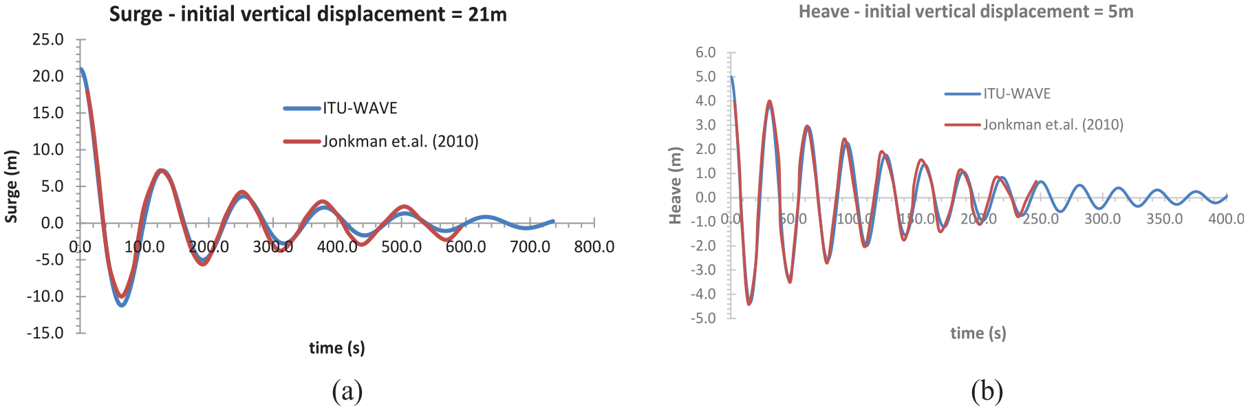
The present paper uses a 5 MW reference wind turbine (Jonkman et al., 2009) for the numerical predictions of the aerodynamic, aeroelastic, hydrodynamic parameters and motion characteristics of FOWT. Figure 3(a) shows free decay time domain simulation of spar buoy surge mode with initial vertical displacement of 21 m whilst the free decay simulation of heave mode with initial vertical displacement of 5 m is presented in Figure 3(b). The free decay simulations in surge and heave modes are obtained using equation (1) where the external forces $F_j^E(t)$ in equation (1) to excite the floater do not exist and considered zero. The present in-house ITU-WAVE free decay simulation numerical results in surge and heave modes are compared with those of Jonkman and Musail (2010) for validation purpose which shows satisfactory agreements. It is important to conduct free decay test as the natural periods of the floater can be directly determined with free decay test at any mode of motion. In addition, the correct wave damping that is produced by the floater can be also checked through free decay test which plays significant role for the decay of the motions at any modes.

Figure 3.

Spar buoy free decay time domain simulation test: (a) surge response and (b) heave response.

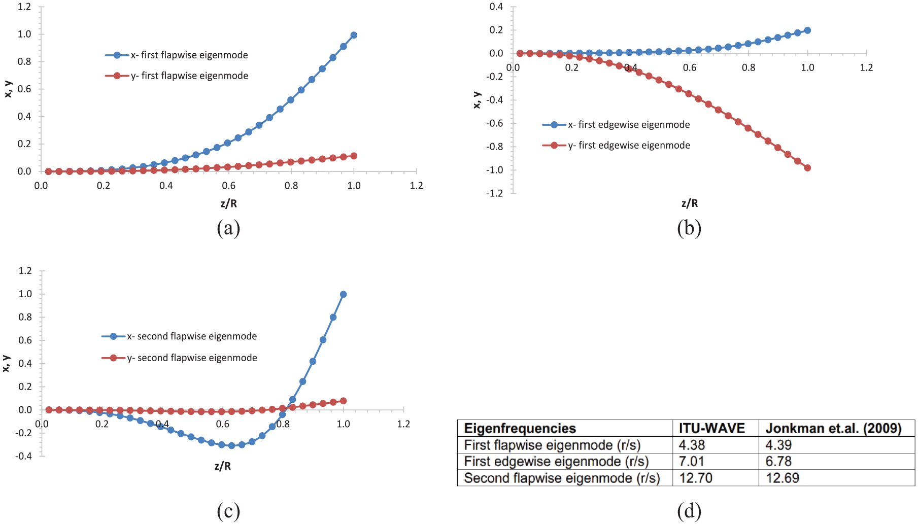
The blades of FOWT are considered as an elastic structure and aeroelastic analysis is applied considering blades as a cantilever beam (Hansen, 2008). The first three eigenmodes of first flapwise, first edgewise and second flapwise eigenmodes, which are predicted using free vibration without the effects of the external applied loads, are presented in Figure 4(a) to (c) respectively. In addition, the first three eigenfrequencies, which are obtained with iterative solutions converging to the lowest eigenfrequencies, are also presented in Figure 4(d). The predicted in-house ITU-WAVE numerical results are compared with those of Jonkman et al. (2009) for the validation of the present numerical results which show satisfactory agreement.

Figure 4.

Eigenmodes and eigenfrequencies: (a) first flapwise eigenmodes, (b) first edgewise eigenmodes, (c) second flapwise eigenmodes and (d) eigenfrequencies.

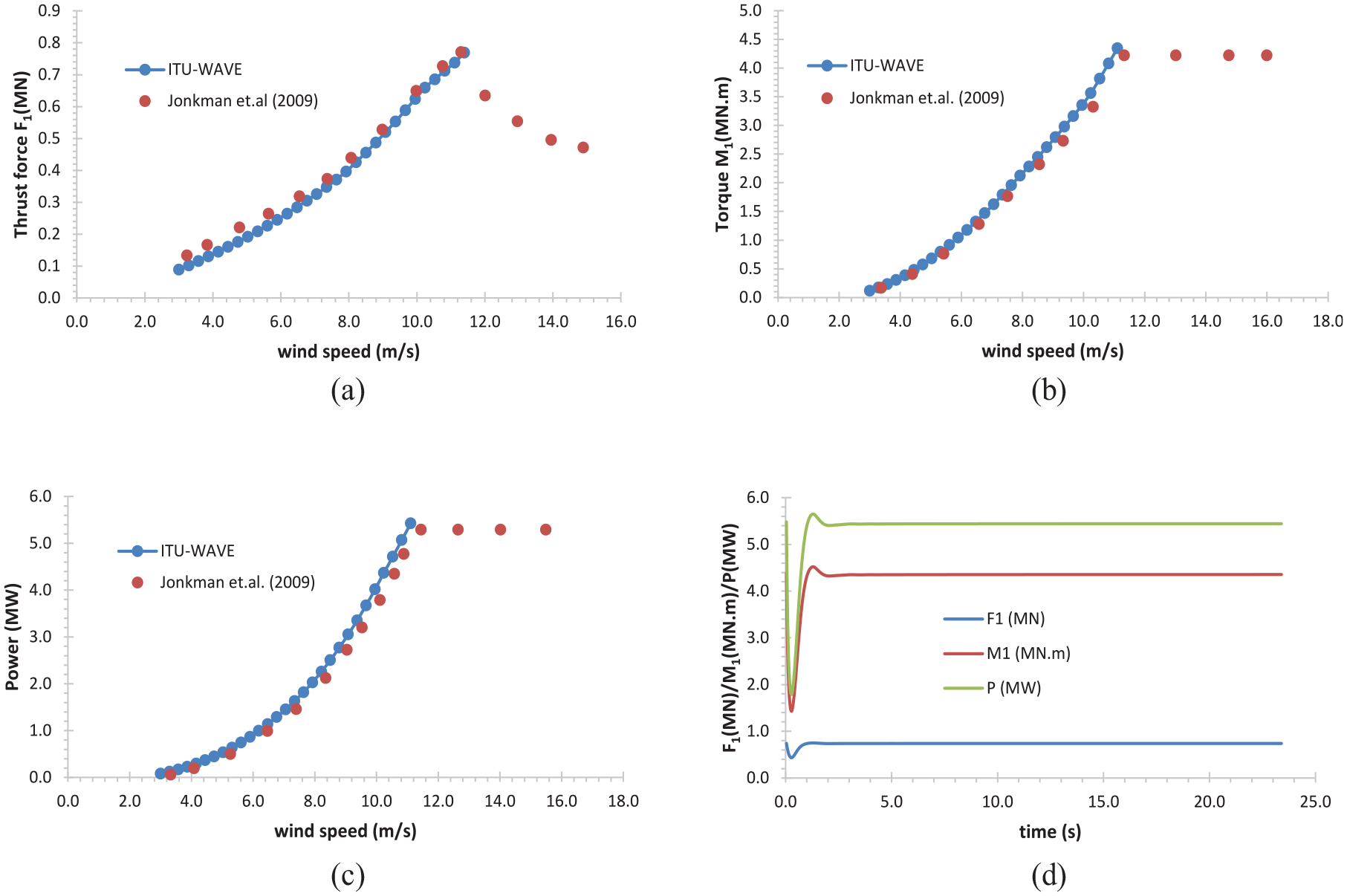
Figure 5(a) to (c) show mean rotor thrust force, torque moment and generated rotor power from wind kinetic energy of the wind respectively with respect to in a range of mean wind speed whilst the time domain simulation of rotor thrust force, torque and power are presented in Figure 5(d) at rated wind speed of 11.4 m/s. The present numerical results of the in-house ITU-WAVE computational tool are obtained using aerodynamic analysis that is presented in section 2.1.1–2.1.3. It can be observed from Figure 5(d) that the time domain simulation length is long enough to avoid transient effects on predicted aerodynamic parameters and only last half of the time domain simulations as presented in Figure 5(d) is used to predict the mean values of rotor thrust force, torque and power in a range of wind speeds. The present numerical results of ITU-WAVE computational tool and those of Jonkman et al. (2009) show satisfactory agreement in Figure 5(a) to (c). It is assumed in the present numerical predictions that the rotor speed and wind speeds are linearly dependent in the region of cut-in wind speed of 3 m/s and rated wind speed of 11.4 m/s. This assumption also results in to have constant tip-speed ratio and optimum conversion efficiency between wind and power output. It can be also observed from Figure 5(b) that rotor torque increases quadratically with respect to wind speed in the region of cut-in speed and rated wind speed whilst rotor power increase cubically at the same region in Figure 5(c).

Figure 5.

(a) Mean thrust force, (b) mean torque, (c) mean rotor power and (d) time domain simulation of thrust force, torque and power at rated wind speed of 11.4 m/s.

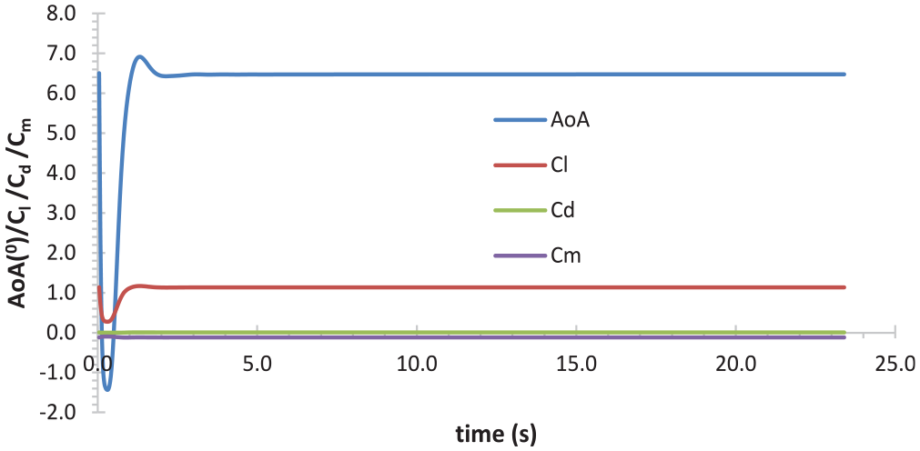
Figure 6 shows the time domain simulation of the aerodynamic parameters of angle of attack ( $\alpha$ ), lift coefficient ( $C_l$ ), drag coefficients ( $C_d$ ) and pitching moment ( $C_m$ ) for the aerofoil at blade tip and rated steady mean wind speed of 11.4 m/s. The present ITU-WAVE numerical results of the aerodynamic parameters are obtained using aerodynamic analysis that is presented in section 2.1.1–2.1.3. As it can be observed from Figure 6, all aerodynamic parameters achieved the steady state condition after 5 seconds whilst the transient effects are died out just after approximately 1 second. It is known that HAWT works best at lower angle of attack ( $\alpha$ ) and present result of approximately $\alpha =6.5^0$ of angle of attack complies with this assumption. It is also correct that the performances of HAWT is greater for maximum wind power generation in the case of at the ratio of maximum lift-drag coefficient. It can be observed from Figure 6 that the present numerical results achieve maximum lift-drag ratio as lift coefficient is around 1.0 whilst drag coefficient is closer to zero for aerofoil at blade tip.

Figure 6.

Time domain simulation of aerodynamic parameters of angle of attack, lift coefficient, drag coefficient and pitching moment at rated steady mean wind speed of 11.4 m/s.

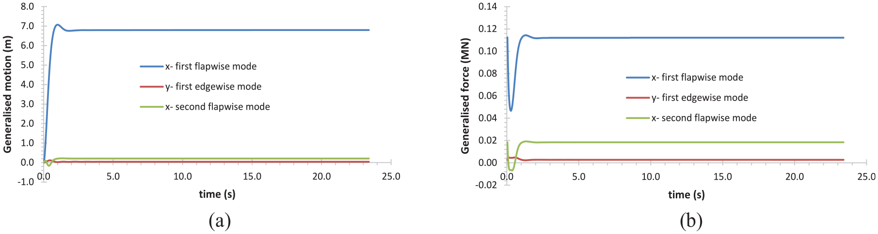
Figure 7(a) and (b) show the time domain simulation of generalised motions and forces at rated mean wind speed of 11.4 m/s including first and second flapwise modes in x-direction and first edgewise mode in y-direction. The generalised motions and forces in Figure 7(a) and (b) are obtained with the time domain simulations of equation (32). When the contribution of first flapwise mode with second flapwise mode for force and motion in Figure 7(a) and (b) is compared, it can be observed that the effect of second flapwise mode is negligible compared to first flapwise mode. It is also correct that the contribution from first edgewise mode to generalised motion and force in y-direction is negligible compared to first flapwise mode in x-direction. It can be concluded from Figure 7(a) and (b) that three modes to get accurate numerical results for generalised motions and forces are enough as the contribution of higher modes would not have significant effects. The time domain simulation shows that after initial transient behaviour, the generalised motions and forces are achieved the steady state condition after 5 seconds.

Figure 7.

Generalised motions and forces in time at rated wind speed of 11.4 m/s: (a) motions and (b) forces.

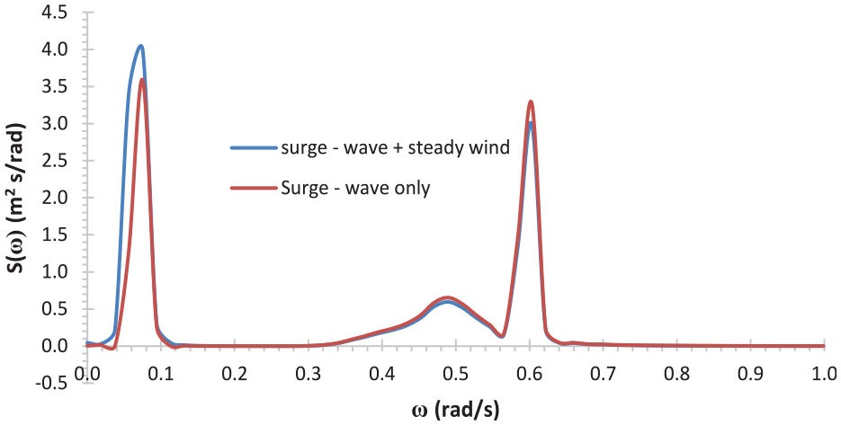
Figure 8 shows surge motion spectrum with and without steady wind speed effect with respect to absolute wave frequency. In the case of surge motion spectrum without steady wind speed, the equation of motion in equation (1) with hydrodynamic analysis including time domain boundary integral equation, Morison equation, mooring analysis of section 2.2 is used to predict surge motion spectrum whilst surge motion spectrum with steady wind speed also includes the aerodynamic analysis of section 2.1. The steady wind speed of $V=8m/s$ is used in the present calculation. The spar buoy floater with diameter at mean water level $D=6.5m$ , diameter at bottom $D=9.4m$ , draft $T=120m$ and water depth of $320m$ in Figure 1 is used to predict surge motion spectrum at wind and wave heading angle of $0^0$ . FOWT is allowed to have motion in only surge mode whilst other modes of motions are restricted. The wave characteristics are described with JONSWAP wave spectrum (Faltinsen, 1990) with significant wave height $H_s=4.2m$ and peak period $T_p=10.5s$ . The first order diffraction forces, viscous forces with Morison equation, forces due to mooring lines and steady aerodynamic wind force in the case of effect of steady wind speed are the external forces on the right-hand-side of equation (1) in the present time domain simulation. The response around $\omega \cong 0.6\mathrm{rad}/s$ represents the wave frequency response whilst the response around $\omega \cong 0.05\mathrm{rad}/s$ shows surge resonant response. When the effects of with and without steady wind speed on surge motion spectrum are compared, it can be observed that steady wind speed effect decreases the amplitudes of incident wave frequency response whilst it increases the amplitude of surge resonant responses slightly and shift it towards lower incident wave frequencies.

Figure 8.

Surge motion spectrum with JONSWAP wave spectrum ${\mathit{H}}_{\mathit{s}}=4.2\mathit{m}$ and ${\mathit{T}}_{\mathit{p}}=10.5\mathit{s}$ with and without wind effect at heading angle $\mathit{\beta }=0^0$ .

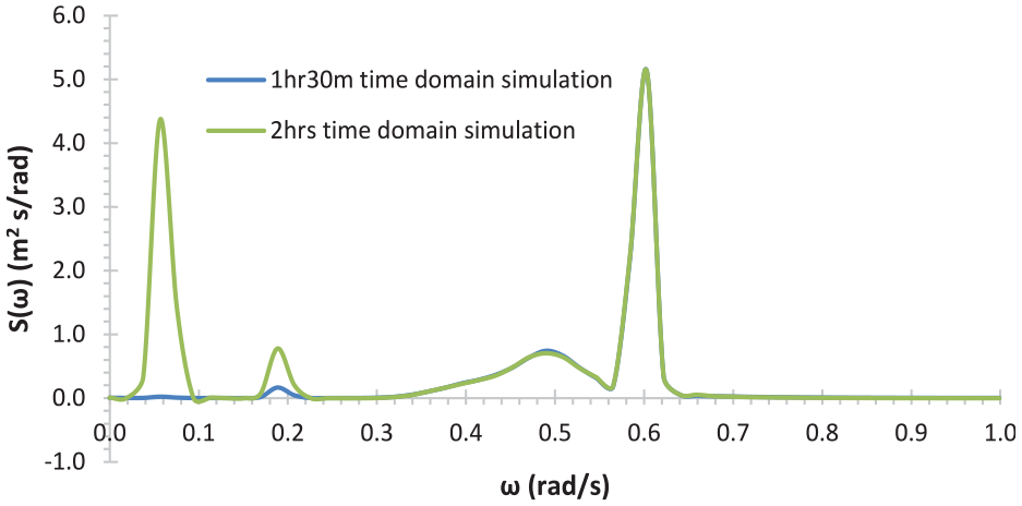
Figure 9 presents the effect of the duration of the time domain simulation on surge motion spectrum with JONSWAP wave spectrum. It is assumed in Figure 9 that there is no wind effect on FOWT which is free in surge and pitch modes whilst the motions are restricted in other modes of the motions. In the case of 1 hour and 30 minutes time domain simulations, although the incident wave frequency response around $\omega \cong 0.6\mathrm{rad}/s$ can be clearly observed which is due to wave load on floater, the surge resonant response around $\omega \cong 0.05\mathrm{rad}/s$ and pitch resonant response around $\omega \cong 0.16\mathrm{rad}/s$ on surge motion spectrum are not clearly felt. However, when the duration of the time domain simulation is increased to 2 hours, the response of the surge resonant and pitch resonant on surge motion spectrum can be clearly seen in Figure 9. It may be noticed that pitch mode has effect on surge motion spectrum. This is due to the coupling of surge motion with pitch motion.

Figure 9.

Effect of duration of time domain simulation on surge spectrum with JONSWAP wave spectrum ${\mathit{H}}_{\mathit{s}}=4.2\mathit{m}$ and ${\mathit{T}}_{\mathit{p}}=10.5\mathit{s}$ without wind effect at heading angle $\mathit{\beta }=0^0$ .

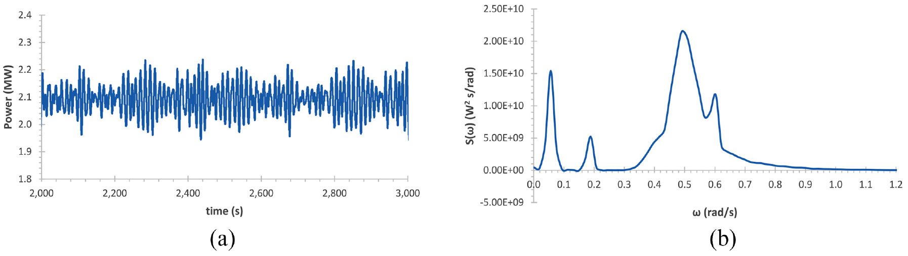
As it can be observed in Figure 10(a), the generated rotor power achieves the steady state condition around 2.1 MW. Power spectrum is presented in Figure 10(b), which is the spectral representation of Figure 10(a) in frequency domain for the same wave and wind conditions. It can be observed from Figure 10(b) that wave frequency response happens around incident wave frequencies of $\omega \cong 0.6\mathrm{rad}/s$ and $\omega \cong 0.5\mathrm{rad}/s$ whilst surge and pitch resonant responses happen at incident wave frequencies of around $\omega \cong 0.05\mathrm{rad}/s$ and $\omega \cong 0.16\mathrm{rad}/s$ respectively.

Figure 10.

Wind power generation with JONSWAP wave spectrum ${\mathit{H}}_{\mathit{s}}=4.2\mathit{m}$ and ${\mathit{T}}_{\mathit{p}}=10.5\mathit{s}$ , steady wind speed of $\mathit{V}=8\mathit{m}/\mathit{s}$ at heading angle $\mathit{\beta }=0^0$ : (a) power and (b) power spectrum.

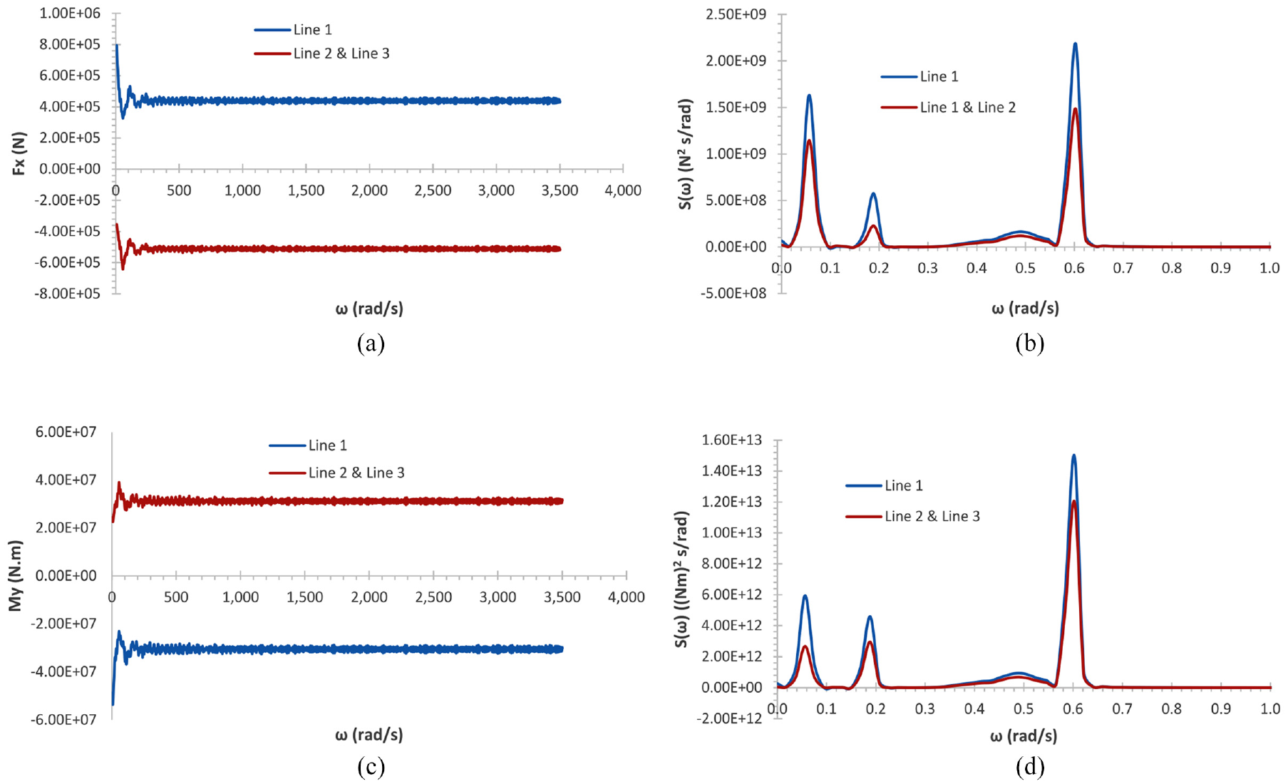
The force and moment on mooring lines with wind and heading angle of $\beta =0^0$ , JONSWAP wave spectrum and steady wind speed in surge and pitch modes are presented in Figure 11(a) and (c) respectively. The force and moment on mooring line 1 and line 3 equal each other due to symmetry of lines with respect to heading angle of $\beta =0^0$ as shown in Figure 11. It can be also observed that surge forces and pitch moment achieve steady state condition over time. Figure 11(b) and (d) show the surge force and pitch moment spectrums. The effects of wave frequency at around peak frequency ( $\omega \cong 0.6\mathrm{rad}/s$ ), surge ( $\omega \cong 0.05\mathrm{rad}/s$ ) and pitch ( $\omega \cong 0.16\mathrm{rad}/s$ ) resonance frequencies can be observed clearly in Figure 11(b) and (d). The amplitude of mooring line 1 in both surge and pitch modes is greater than mooring line 2 and line 3. It is also clear that the influence of wave frequency compared to surge and pitch resonant frequencies to the surge force and pitch momentum spectrum is greater whilst the effects of surge resonant frequency is greater than pitch resonant frequency both in surge force and pitch moment spectrums.

Figure 11.

Force and moments on mooring lines with JONSWAP wave spectrum ${\mathit{H}}_{\mathit{s}}=4.2\mathit{m}$ and ${\mathit{T}}_{\mathit{p}}=10.5\mathit{s}$ , steady wind speed of $\mathit{V}=8\mathit{m}/\mathit{s}$ at heading angle $\mathit{\beta }=0^0$ : (a) surge force, (b) surge force spectrum, (c) pitch moment and (d) pitch moment spectrum.

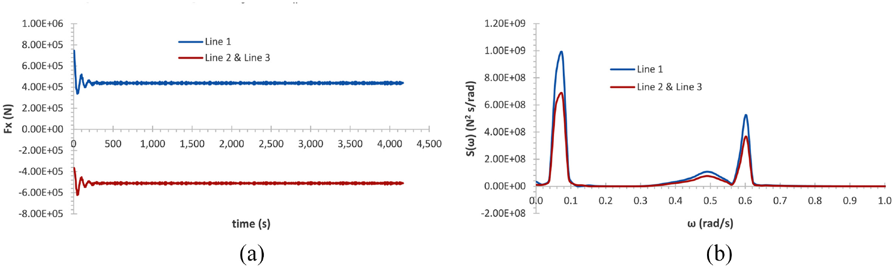
Figure 12(a) shows the surge force on mooring line due to only surge motion with steady wind speed of $V=8m/s$ and JONSWAP wave spectrum at wind and heading angle $\beta =0^0$ whilst the surge force spectrum on mooring lines is presented in Figure 12(b). When Figures 11(b) and 12(b) are compared, the amplitudes of surge force spectrum on mooring lines considerably reduced in the case of effect of only surge mode in Figure 12(b). It can be also observed in Figure 12(b) that effect of surge resonant frequency around $\omega \cong 0.05\mathrm{rad}/s$ is greater compared to that of wave frequency around $\omega \cong 0.6\mathrm{rad}/s$ . As the pitch mode of motion is restricted, there is no response around $\omega \cong 0.16\mathrm{rad}/s$ in Figure 12(b) which is pitch resonant frequency. The amplitude of the surge force spectrum on mooring line 1 is greater than that of mooring lines 2 and 3 which have the same spectrum due to the symmetric configurations of mooring line 2 and line 3 with respect to wind and incident wave heading angle $\beta =0^0$ .

Figure 12.

Surge force and force spectrum on mooring lines with JONSWAP wave spectrum ${\mathit{H}}_{\mathit{s}}=4.2\mathit{m}$ and ${\mathit{T}}_{\mathit{p}}=10.5\mathit{s}$ , steady wind speed of $\mathit{V}=8\mathit{m}/\mathit{s}$ at heading angle $\mathit{\beta }=0^0$ : (a) surge force and (b) surge force spectrum.

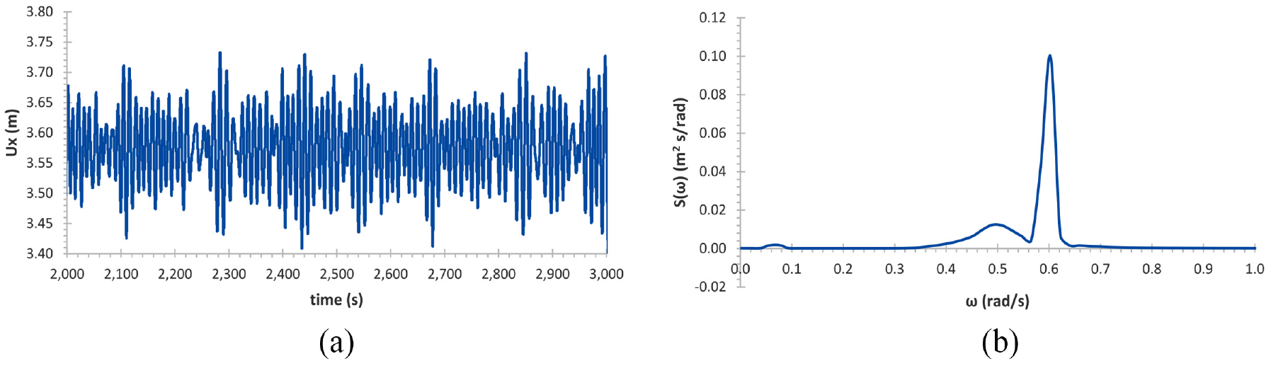
Figure 13(a) and (b) shows the blade tip deflection and blade tip deflection spectrum respectively with steady wind speed of $V=8m/s$ and JONSWAP wave spectrum. FOWT is free in surge mode whilst it is restricted in other modes of motions. The effect of wave frequency around $\omega \cong 0.6\mathrm{rad}/s$ on blade tip deflection spectrum can be observed clearly in Figure 13(b) whilst the surge resonant response around $\omega \cong 0.05\mathrm{rad}/s$ does not have significant response amplitude.

Figure 13.

Blade tip deflection with JONSWAP wave spectrum ${\mathit{H}}_{\mathit{s}}=4.2\mathit{m}$ and ${\mathit{T}}_{\mathit{p}}=10.5\mathit{s}$ , steady wind speed of $\mathit{V}=8\mathit{m}/\mathit{s}$ at heading angle $\mathit{\beta }=0^0$ : (a) blade tip deflection in time and (b) blade tip deflection spectrum.

Conclusions

ITU-WAVE in-house computational tool is used to predict the aerodynamic, aeroelastic, hydrodynamic parameters and wind power generation with FOWT. The hydrodynamic diffraction and radiation force variables including free decay tests are predicted with the solution of the time domain boundary integral equation and Morison equation which is used to approximate the viscous effect. The aerodynamic parameters are predicted with unsteady BEM method which also include the effects of the dynamic stall and dynamic inflow. The aeroelastic behaviour of FOWT’s blades are considered with the first three elastic modes. In addition, the forces on the wind turbine tower, which is considered as a rigid structure, are predicted with average wind factor.

The effects of wave and steady wind on motion spectrum show that although the steady wind contributes to the motion spectrum, its influence is not greatly changing the behaviour of the motion spectrums. The influences and effects of wave frequency, and surge and pitch resonant frequencies on motion spectrums, mooring lines spectrums and blade tip deflection spectrum depend considerably on the duration of the time domain simulation. The numerical experiences also show that the numerical results need over 2 hours simulation time to feel the effect of the surge and pitch resonant frequencies on motion spectrums whilst the influence of the wave frequency needs much less simulation time.

The present in-house transient ITU-WAVE predicted numerical results are validated against other numerical results including the eigenfrequencies of wind turbine blades which is considered as an elastic cantilever beam. In addition, the achieving steady state results of thrust force, torque moment and rotor power are also validated with other numerical results which show satisfactory agreements. The aerodynamic parameters with time domain simulation are predicted by taking only last half of the time domain simulation into account to avoid the transient effects. The free decay tests of pitch and surge modes are also validated with other published numerical results which are also in good agreements with other numerical results.