
Abstract
A method for structural analysis of thin-walled composite beams like wind turbine blades is presented. This method is based on the Nonhomogeneous Anisotropic Beam Section Analysis (NABSA) which consists in discretizing the beam cross section using finite elements. The proposed implementation uses 3-node line cross-sectional finite elements with nodes having rotational degrees of freedom to describe the cross-sectional warping displacements. Solutions obtained using this approach were verified against the corresponding analytical or numerical solutions. Agreement was very good to excellent for the computation of cross-sectional properties and distribution of stresses, strains and warping displacements for a broad range of possible composite beam behaviors including geometric and material couplings, open sections, multicell sections, and arbitrary laminates. For thin-walled layered structures, the proposed method provides models with fewer degrees of freedom than equivalent models based on a two-dimensional discretization of cross sections using triangular or quadrilateral elements such as conventional NABSA or VABS which suggests that computation time could be reduced.
Keywords
Introduction
Wind turbine blades, as well as airplane wings and helicopter rotor blades, are mostly composite beams. Unlike classical metallic structures, these composite beams have cross-sectional non-homogeneity and offer the possibility of enabling coupling between all deformation modes that may arise from fiber orientation. This latter phenomenon can be used as a load alleviation system, for example when a bend-twist coupling exists in the behavior of a wind turbine blade (Fedorov and Berggreen, 2014). As the structures mentioned earlier are often modeled as beams, especially for aeroelastic analyses, their cross-sectional properties need to be computed. In order to consider all the possibilities associated with composite beams, models more elaborate than the classical strength of material methods applied to homogeneous cross sections are needed.
To develop such models, the Variational Asymptotic Beam Section Analysis available in commercial VABS software is a reference tool (Cesnik and Hodges, 1997; Hodges and Yu, 2007; Yu et al., 2002a, 2002b, 2012).The beam cross section is discretized using two-dimensional finite elements and a 6 × 6 cross-sectional stiffness matrix is calculated. Shear effects are therefore taken into account so the beam can be considered a Timoshenko beam. Giavotto et al. (1983), based on a different methodology, have also developed a tool to compute a 6 × 6 cross-sectional stiffness matrix for a Timoshenko beam using again a two-dimensional finite element discretization of the cross section. This framework is sometimes called Nonhomogeneous Anisotropic Beam Section Analysis (NABSA). This work has been updated in software called BECAS that also includes optimization capabilities (Blasques, 2011; Blasques et al., 2016; Blasques, 2012; Blasques and Stolpe, 2012).
However, as wind turbine blades, airplane wings and helicopter rotor blades are often thin-walled structures, it is possible to use methods based on the theory of strength of materials. Of course, these methods have to be adjusted to take into account the composite nature of these structures. These adjusted methods allow the computation of the cross-sectional stiffness matrix terms by evaluating integrals over the beam cross section based on various deformation hypotheses.
The first distinction that can be made among models based on strength of materials is the way transverse shear effects are taken into account. Formulations based on Timoshenko beams include such effects (Fernandes da Silva et al., 2011; Librescu and Song, 2006; Massa and Barbero, 1998; Pluzsik and Kollar, 2002; Saravanos et al., 2006; Saravia, 2014; Saravia et al., 2012; Sheikh and Thomsen, 2008; Zhang et al., 2012) whereas those based on Euler beams ignore them (Cárdenas et al., 2012; Cardoso et al., 2009; Gökhan Günay and Timarci, 2017; Kollar and Pluzsik, 2002; Victorazzo and De Jesus, 2016; Wang and Zhang, 2014; Wang et al., 2014; Zhang and Wang, 2014).
In both of these cases, different ways to model the torsional behavior of the beam are used. Some authors build their model based on uniform torsion, that is, Bredt theory for thin-walled beams (Fernandes da Silva et al., 2011; Kollar and Pluzsik, 2002; Saravanos et al., 2006; Saravia, 2014; Saravia et al., 2012; Victorazzo and De Jesus, 2016; Wang et al., 2014; Zhang et al., 2012). This means that the beam has a constant section loaded by torques at the ends only and that support effects are neglected. However, this theory is still valid for slightly variable cross sections and slightly variable distributed torques as well as for sections away from the effects of supports. Other models are based on non-uniform torsion, that is, Vlasov torsion, where variable cross section, variable torque distribution or support effects cause restraint to the out-of-plane warping of the cross section (Cárdenas et al., 2012; Cardoso et al., 2009; Gökhan Günay and Timarci, 2017; Librescu and Song, 2006; Massa and Barbero, 1998; Pluzsik and Kollar, 2002; Sheikh and Thomsen, 2008; Wang and Zhang, 2014; Zhang and Wang, 2014). According to Volovoi and Hodges (2000) and Yu et al. (2005), the Vlasov correction for restrained warping has been found unnecessary for closed thin-walled beam as this effect has minimal impact on that kind of structure.
Among the cited models, some are able to consider general composite plate stacking sequences along with all coupling implied (Cárdenas et al., 2012; Gökhan Günay and Timarci, 2017; Kollar and Pluzsik, 2002; Librescu and Song, 2006; Pluzsik and Kollar, 2002; Saravanos et al., 2006; Saravia, 2014; Saravia et al., 2012; Sheikh and Thomsen, 2008; Victorazzo and De Jesus, 2016; Wang and Zhang, 2014; Zhang and Wang, 2014). This allows modeling of the bend-twist coupling of the beam. With some exceptions (Cárdenas et al., 2012; Cardoso et al., 2009; Fernandes da Silva et al., 2011; Wang et al., 2014; Zhang et al., 2012), these models take into account wall bending rigidity.
All the cited models can be used to evaluate closed single-section beams. Some are also able to model open section beams (Cardoso et al., 2009; Kollar and Pluzsik, 2002; Librescu and Song, 2006; Massa and Barbero, 1998; Pluzsik and Kollar, 2002; Sheikh and Thomsen, 2008; Victorazzo and De Jesus, 2016; Zhang et al., 2012) and others, closed multicell section beams (Cárdenas et al., 2012; Fernandes da Silva et al., 2011; Pluzsik and Kollar, 2002; Victorazzo and De Jesus, 2016; Wang and Zhang, 2014; Wang et al., 2014; Zhang et al., 2012).
Coming back to the more complex VABS and NABSA methods, the modeling of thin-walled cross section with these tools (using line finite elements instead of 2D finite elements) is also interesting. Thin-walled implementations of the VABS method have already been proposed. Some are based on classical Euler beam model with (Yu et al., 2005) or without (Volovoi and Hodges, 2000, 2002) the Vlasov correction. Others are based on Timoshenko beam model (Ferede and Abdalla, 2014; Gupta and Hodges, 2017).
The contribution of this paper is a thin-walled implementation of the theory behind NABSA. This leads to a
In the following sections, we review the literature relevant to classical NABSA theory and then describe the proposed finite-element implementation of our method, which we verify by comparison with analytical and numerical (using 3D shell finite elements) solutions.
Review of the theory underlying NABSA
This section presents the NABSA theory as developed by Giavotto et al. (1983) and extended for optimization by Blasques and Stolpe (2012), Blasques (2012, 2011) and Blasques et al. (2016). The nomenclature adopted in this article is similar to that used by the latter group. In this theory, it is assumed that the beam is straight, has a constant cross section and is loaded at its ends only.
Coordinate systems
Figure 1 shows the different coordinate systems used: a global coordinate system
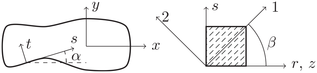
The coordinate systems used in this study.
Stress and strain
The stress and strain components are used in a vectorial form defined as

and the stress-strain relationship is

where

Internal loads
The beam internal load vector is defined as

where

where

Generalized strain
Defining the beam reference axis displacements

and defining the Timoshenko beam generalized strains as

It can be shown that

where
and the prime symbol (’) denotes a first derivative with respect to
Kinematics of the cross section
The displacement of an arbitrary point in the cross section

The term
Strain-displacement relationships
By separation of the derivative with respect to

where
Using equations (11) and (9), given that

Finally, the warping function

where

Principle of virtual work for a beam slice and solution
Based on the virtual work (per unit length of the beam) of a beam slice

Giavotto et al. (1983), Blasques and Stolpe (2012), Blasques (2012, 2011) and Blasques et al. (2016) show that the following system is obtained for the center of the beam (far from the boundary conditions):
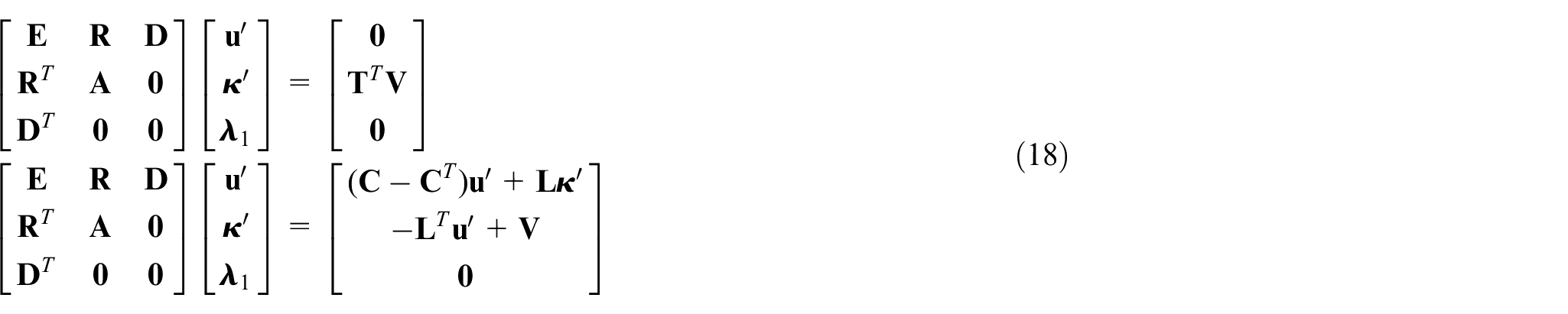
Given the internal load vector
The

The other matrices needed for equation (18) are defined as
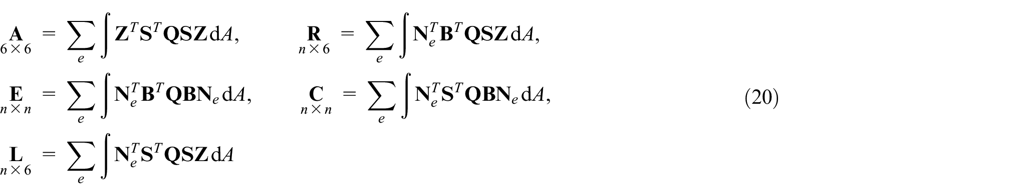
where
Cross-sectional stiffness matrix
To get the beam cross-sectional stiffness matrix

The simplest way to proceed is to choose
Note that this method of computing the beam cross-sectional stiffness matrix differs from that used by Giavotto et al. (1983), Blasques and Stolpe (2012), Blasques (2012, 2011), and Blasques et al. (2016),which was based on the principle of virtual work.
Implementation of the line finite element
In order to be able to perform a cross-sectional analysis, the matrices of equation (20) have to be evaluated. This section presents the procedure for the computation of a general
Shape functions and element coordinate system at nodes
Figure 2 shows an example of real and reference elements for a 3-node line element. The
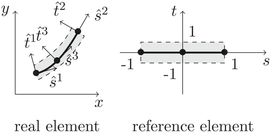
Real and reference elements (example for
Coordinate of a point in the element
The
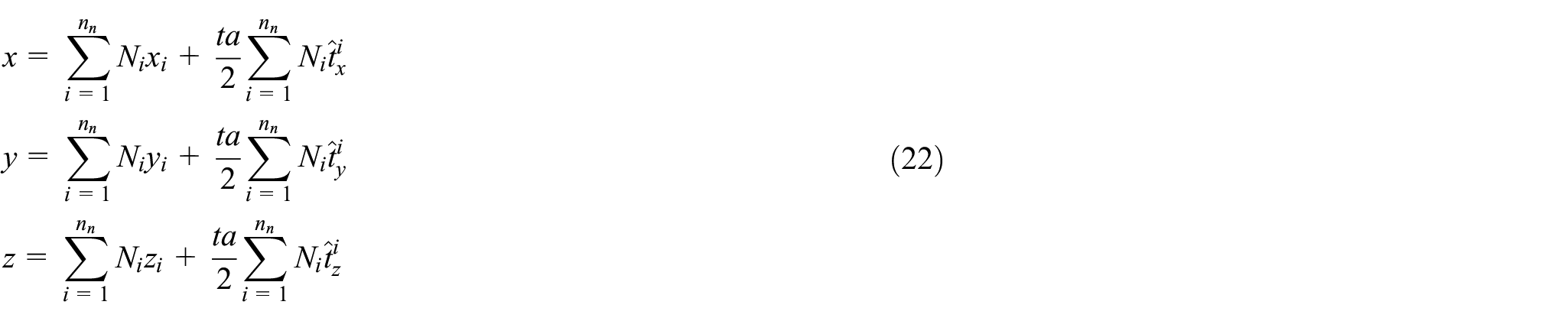
where
Jacobian matrix
The Jacobian matrix
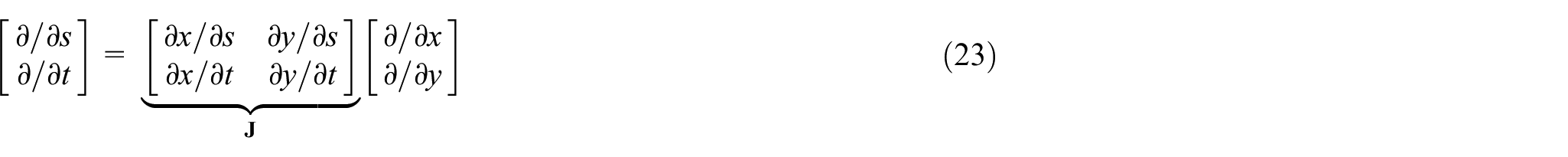
Using equation (22), this matrix can be expressed as follows:

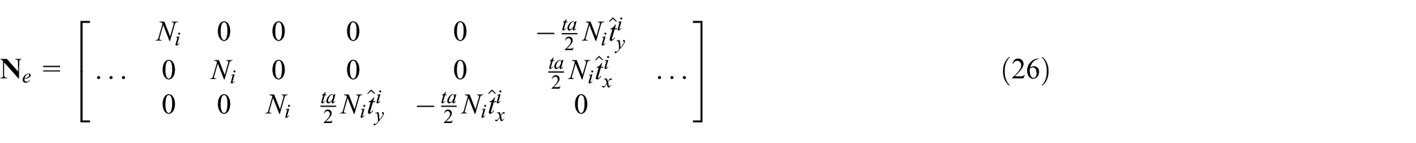
Displacement field, shape function and derivative of shape function matrices
The displacement field can be evaluated by subtracting the final and initial positions of each node using equation (22) (Bathe, 2006).The warping displacement field is then:

where the shape function matrix is
The nodal displacement vector is

Differentiating the shape function matrix using equation (23) yields:
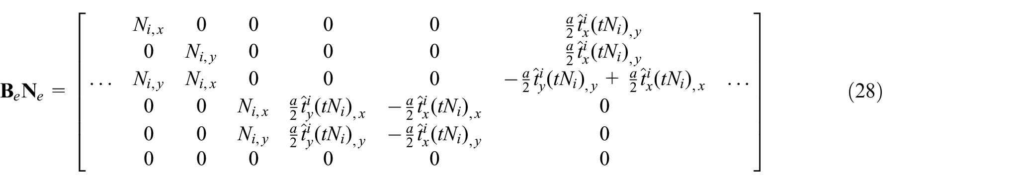
where

and
Material properties
Since the stress–strain relationship of the material must be expressed in the global coordinate system (
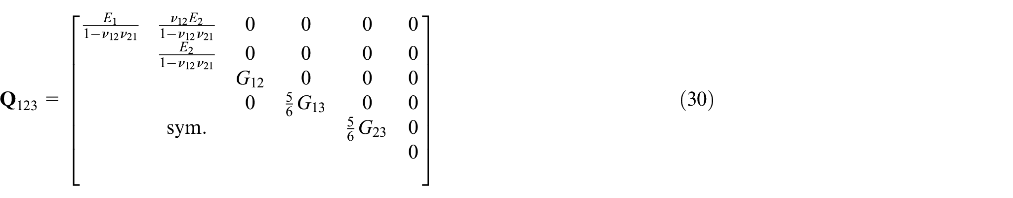
where
The transformation of the constitutive matrix to the global coordinate system is achieved in two steps. The first step consists of a transformation in the element coordinate system:

and the second step, in the global coordinate system:

for which the transformation matrices
Numerical integration
The integration of equation (20) over the area of the elements is computed numerically using Gauss formula. A full integration is used in the
Fictitious rigidity for drilling degrees of freedom
Since no stiffness is associated with the node drilling degree of freedom (rotation about the
Post-processing
For a given load case, once the nodal displacements
The stresses and strains can be computed in the element and material coordinate systems as:

The shell internal loads can then be computed as integrals of the stress components over the element thickness:

for
Implemented elements
For the verification presented in the next section, a three-node element (
Verification of the implemented element
This section proposes different verification cases intended to verify the performance of the proposed method for the analysis of different types of nonhomogeneous anisotropic thin-walled beams. The pre- and post-processing of the models is done with the Gmsh software (Geuzaine and Remacle, 2009). Note that all the gradient results presented (stresses, strains and shell internal loads) are computed at the center of the element, that is, at
Concerning computation time, the proposed model being coded using Python, all matrices assembly and derived result calculations are done using scripts in an interpreted language (slow) and solution of the equation system is done using a compiled function (fast). It is therefore impossible to get realistic computation time data to compare to the 2D cross-sectional discretization. However, we can suppose that the 1D proposed model will result in smaller computation times for cross section using laminated wall with several layers. 2D models need one element per layer through the thickness, while the proposed 1D model needs only one node through the thickness, resulting in a model with fewer degrees of freedom.
The results presented in the next sections are shown dimensionless but use the International System of Unit: lengths, forces and stresses are respectively in m, N and Pa.
Preliminary verification cases
Some preliminary verification tests on circular and rectangular thin-walled homogeneous sections have shown that the proposed model is able to correctly manage these kinds of problems. All components of the cross-sectional stiffness matrices are the same as the corresponding analytical solutions. For the computation of the analytical transverse shear behavior, the Cowper (1966) shear correction factor is used because it is defined for static analysis such as the one performed here. Stress and strain values returned by the proposed model are also correct.
A convergence analysis has been performed on a homogeneous thin-walled circular cross section of radius
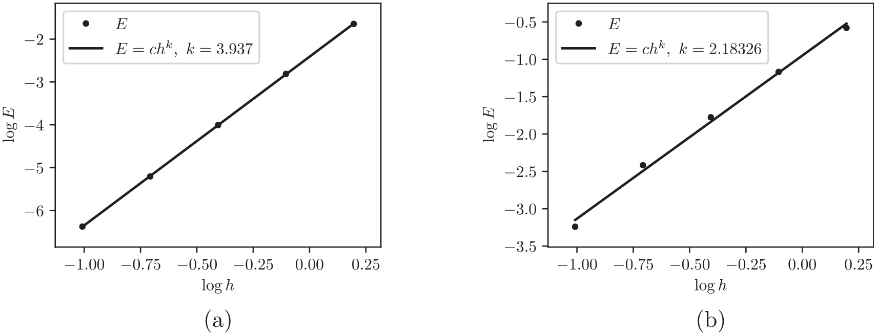
Convergence rate of: (a) torsion cross-sectional stiffness
Based on this same thin-walled circular cross section, it is also interesting to study how the proposed model performs when the shell thickness is increased. Figure 4a compares the transverse shear cross-sectional stiffness with respect to element thickness for numerical and analytical solutions. Results show that the numerical results match the analytical result even for a solid cross section (
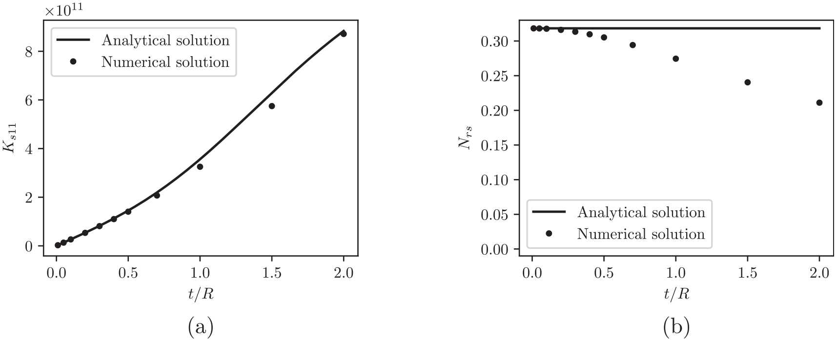
Comparison of the proposed model solution with analytical solution for increasing thickness to the radius ratio. (a) transverse shear cross-sectional stiffness
Verification case 1
For verification case 1, a thin-walled circular cross section of radius
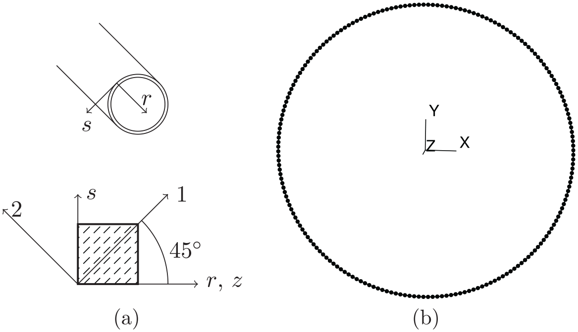
Verification case 1: (a) model geometry and (b) mesh.
The cross-sectional compliance matrix can be obtained analytically by computing the generalized strain vector for six unit internal force load cases. For that analysis, a shear correction factor of 0.5 is used. The resulting compliance matrix is as follows:
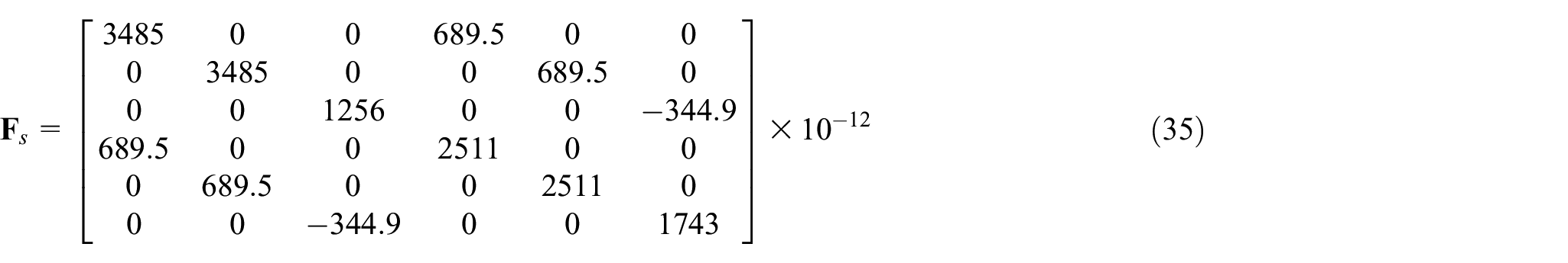
The solution obtained from the proposed model using 100 quadratic elements (mesh shown in Figure 5b) is
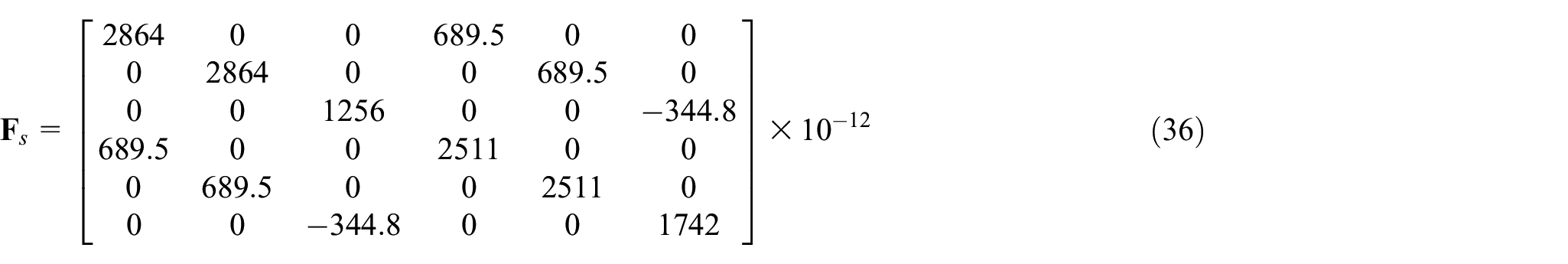
These solutions are very similar, with differences of less than 0.1% except for the transverse shear compliances (
Verification case 2
In this verification load case, we study an open thin-walled section. The cross-sectional shape is the same as verification case 1 excepted that the section is open at the point of coordinate
Using the proposed model with 100 quadratic elements, we obtain the following cross-sectional stiffness matrix:
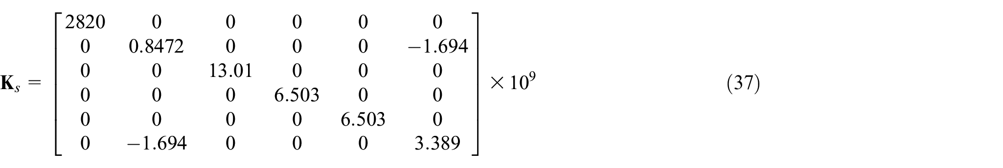
As expected, we can observe a coupling between the shear force in the
and there is now a coupling between the extension and the bending about
As we can see, the torsional stiffness
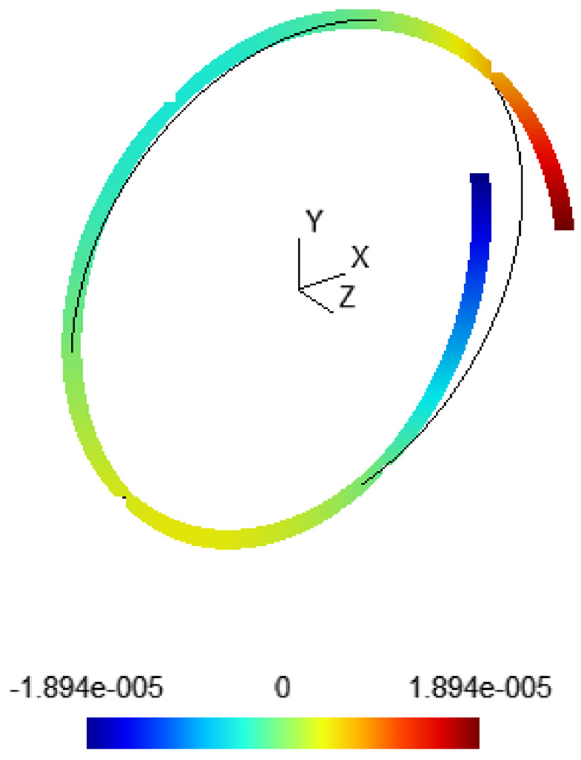
Verification case 2. Warping displacement
All of the differences observed here could be reduced by increasing the number of finite elements in the mesh. This verification case shows that the proposed model correctly manages open sections and geometric shear-torsion coupling.
Verification case 3
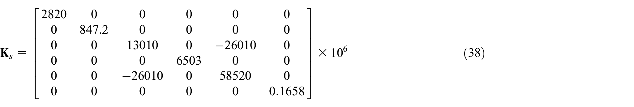
This verification case consists of a thin-walled multicell cross section. The geometry is represented in Figure 7a and the material is the same as verification case 2. The analytical solution to this problem shows that the torsional stiffness of this cross section is
Verification case 3: (a) geometry and (b) shear flow
With 124 quadratic elements, the proposed model locates the shear center at
Verification case 4
In the previous verification cases, the mesh line always represented the middle of the shell thickness. However, the reference geometry is often located on one of the shell surfaces. Wind turbine blades and airplane wings are examples where the reference geometry is the exterior surface. In such cases it may be more useful to be able to build the model in order for the mesh to represent the bottom of the plate, that is, the thickness is built only on one side of the mesh. This can be achieved by integrating in the thickness direction from
By modeling verification case 2 this way, the mesh being located on the outer surface, the predicted shear center location is
The only considerable error is for transverse shear stiffness in the
Verification case 5
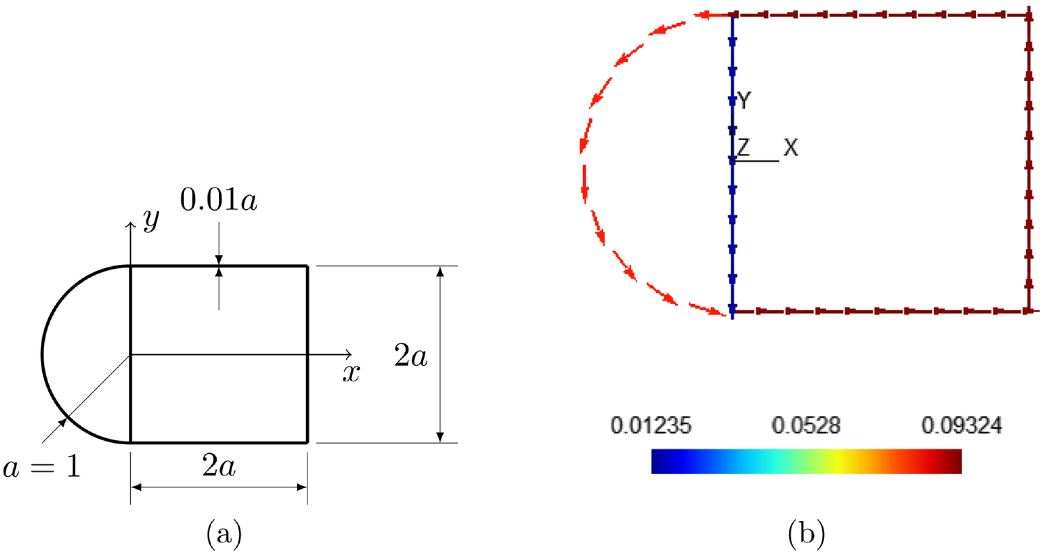
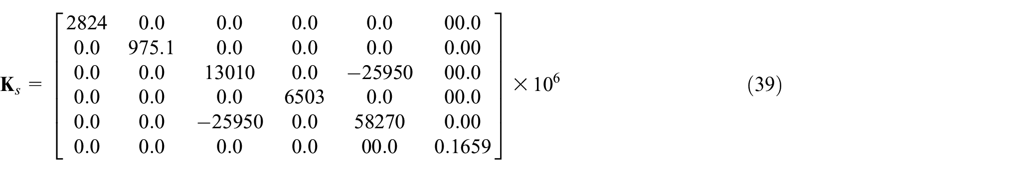
With this verification case, we want to see if the model reacts correctly to a nonsymmetrical and unbalanced layup. Considering the difficulty of obtaining an analytical solution for that kind of layup, the problem studied here consists of a simple plate of unit width in the global
Stress distribution in the plate for verification case 5.
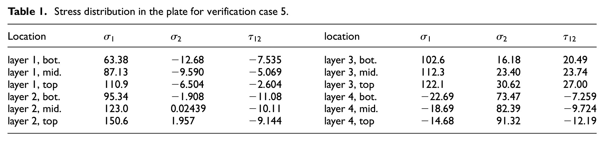
The proposed model gives the same results up to four significant digits. These results are also obtained when using the option to place the nodes at the bottom of the laminate as explained in verification case 4.
Verification case 6
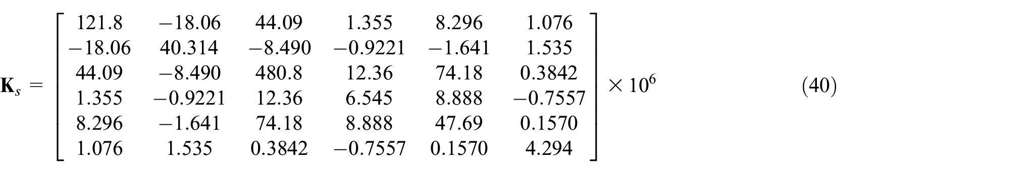
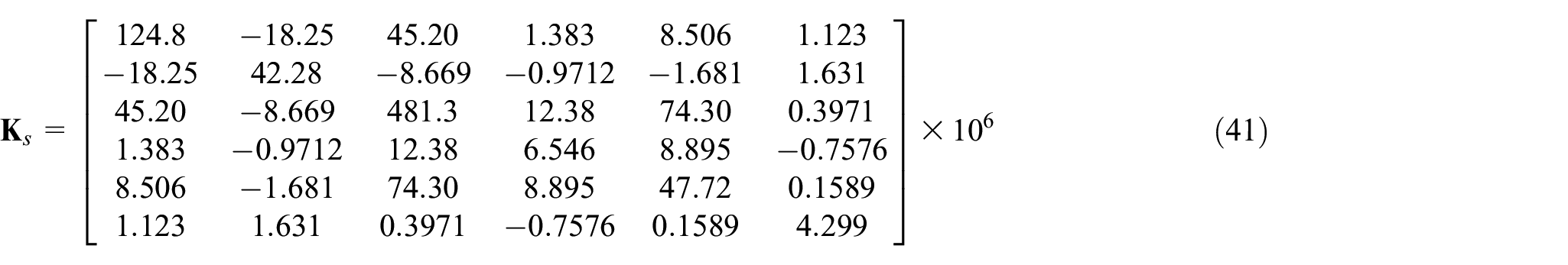
As a final verification case, a nonsymmetrical multicell cross section like that of wind turbine blades is analyzed. As represented in Figure 8a, the cross section uses unbalanced laminates to induce bend-twist coupling (Fedorov et al., 2009). All laminates are centered on the mesh line. So, the nodes of the airfoil contour (laminates 1–4) are shifted toward the interior in order to get the correct geometry. All layers are made of the same material as in verification case 1 with a thickness of 0.001. Using the proposed methodology, when this cross section is meshed using 200 nodes and 101 quadratic elements (see Figure 8b), the resulting cross-sectional stiffness matrix is
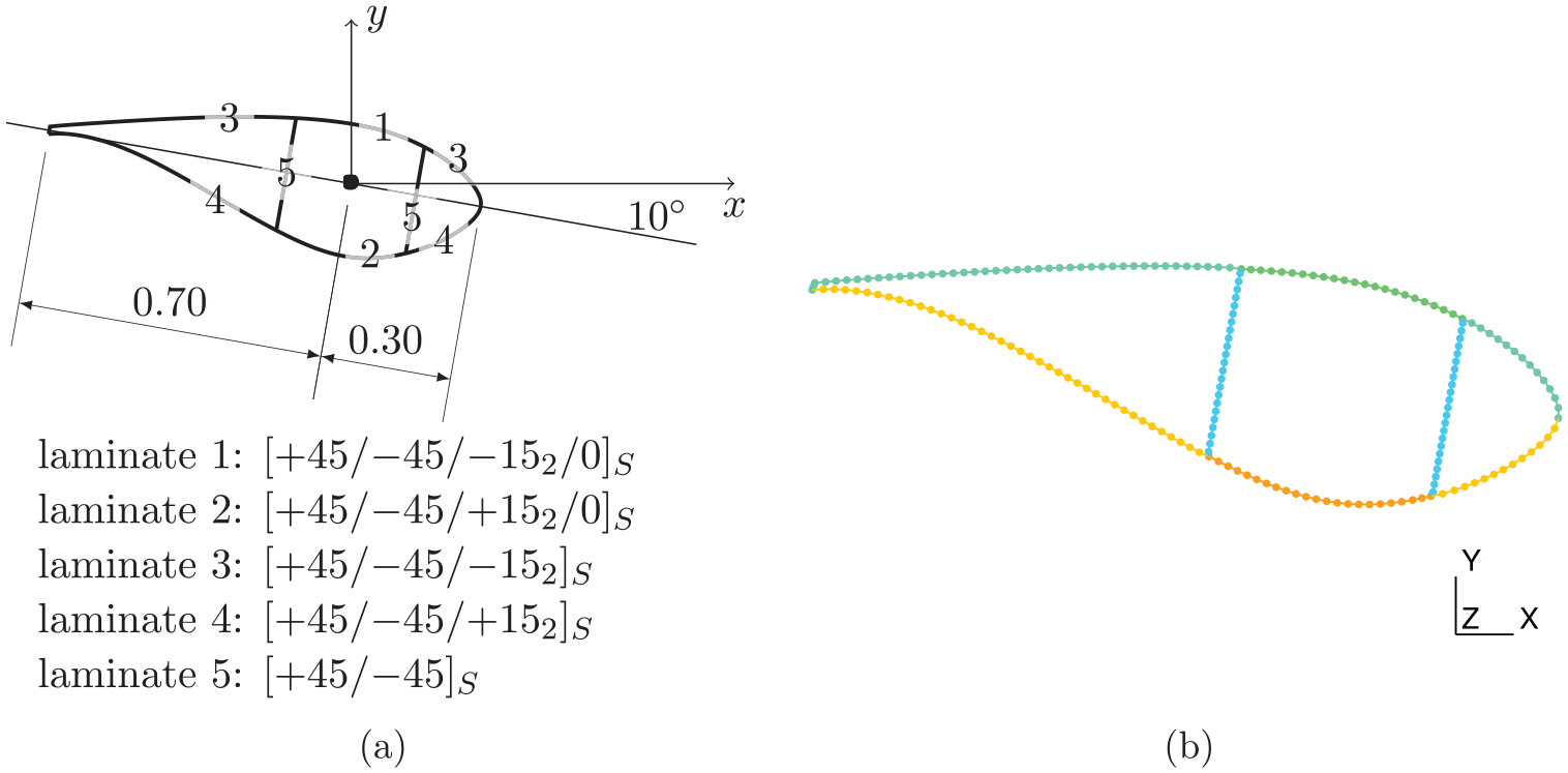
Verification case 6. The airfoil is a DU 97-W-300 (Timmer and van Rooij, 2003). Both shear webs are perpendicular to the airfoil chordline and are located at 0.15 on each side of the origin of the coordinate system. For the airfoil contour (laminate 1–4), the bottom of the laminate is toward the airfoil exterior and the top of the laminates are toward the airfoil interior. For the shear webs, the bottom of the laminates are toward the leading edge and the top of the laminates are toward the trailing edge: (a) geometry and (b) mesh.
These results are compared with those of a 3D shell finite element model of a beam of length 50.0. For that model that uses the Altair OptiStruct solver (see Figure 9), the beam is meshed with 299,200 nodes and 101,000 8-node shell elements (101 in the cross section and 1000 along beam length). RBE2 elements are used at both ends to apply loads and supports. The cross-sectional stiffness matrix resulting from this 3D shell finite element model is as follows:
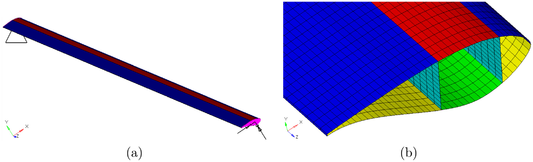
3D shell finite element model of verification case 6: (a) full model and (b) close-up.
These results are obtained by computing the displacements and rotations of groups of nodes at different cross section and differentiate these distributions with respect to the longitudinal axis. This methodology is presented in Forcier and Joncas (2022).
When comparing both models, the differences are (absolute value of the difference normalized by the average of both values):
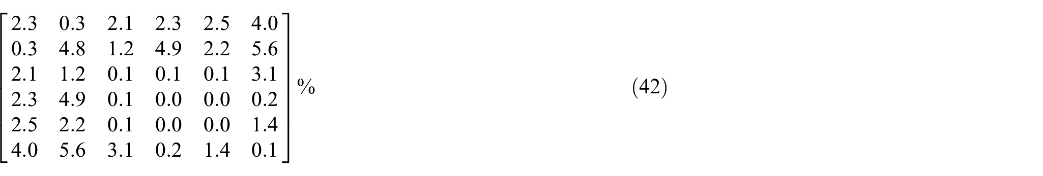
For the extension-bending behavior (
Figure 10 shows the warping displacement results under a torsional load for both of these models. The warping displacement fields are very similar on both models and the extreme values are within a 5% difference range.
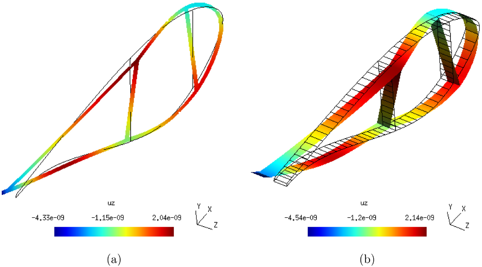
Verification case 6: Warping displacement
Finally, it is interesting to compare these results with those obtained when using offset nodes on the airfoil contour (nodes on the outside surface and thickness built toward the interior). When using the proposed model, the differences with the solution obtained with mid-surface nodes (equation (40)) are
The difference for extension and bending is small, being limited to 1.4%. When looking at transverse shear and torsion, the differences are higher but limited to 10%. Higher error values are experienced for coupling terms of lower importance (
When comparing the difference between the mid-surface node solution (Eq. 41) and the offset node solution of the 3D shell finite element model, the extension and bending behavior are still correctly modeled, but the error is now 36% on the torsional stiffness (
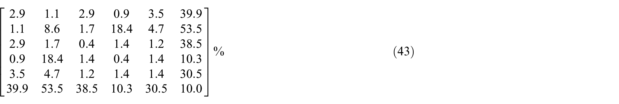
It is interesting to note that the proposed cross-sectional finite element model is less affected by this problem than 3D shell finite elements. Furthermore, as suggested by Tavares et al. (2022), increasing the drilling degree of freedom stiffness reduces the error. In this particular case, the difference between the offset node solution and the mid-surface node solution resulting from the proposed cross-sectional finite element model presented in equation (43) can be reduced to maximum values of 1.4% for extension and bending terms (
Conclusion
In this paper, a thin-walled implementation of the Nonhomogeneous Anisotropic Beam Section Analysis (NABSA) method has been proposed using a finite element formulation similar to the pure displacement formulation used for shell elements. After a recall of the NABSA method, its thin-walled implementation was presented for a general
A 3-node element implementation was then verified against different cases for which an analytical or numerical solution was obtained. These verification cases covered a broad range of possible composite beam behaviors: geometric coupling, material couplings due to off-axis fiber, open sections, multicell sections, nodes located on the shell bottom surface, nonsymmetrical, and unbalanced laminates. The results obtained from the proposed model showed very good agreement with the analytical and numerical solutions.
The proposed method allows the computation of the beam cross-sectional stiffness matrix as do the classical NABSA or VABS methods does, but facilitates model construction by providing a natural through-the-thickness direction to define the material coordinate system. It also facilitates the computation of the stresses and strains in different laminate layers and of shell internal loads (such as shear flow, for instance). Finally, it provides models that are smaller and compute faster than do classical NABSA or VABS methods using two-dimensional discretization of cross sections with triangular or quadrangular elements.
Footnotes
Declaration of conflicting interests
The author(s) declared no potential conflicts of interest with respect to the research, authorship, and/or publication of this article.
Funding
The author(s) disclosed receipt of the following financial support for the research, authorship, and/or publication of this article: This work was supported by the Fonds québécois de la recherche sur la nature et les technologies (FQRNT, Quebec, Canada) [Doctoral research scholarships, B2].