Calculating loads and life-time reduction of wind turbine gearbox and generator bearings due to shaft misalignment

Abstract

During the last two decades, wind turbine industries have faced high failure rates, downtimes and costly repairs. Gearbox and generator have contributed to this, especially, because their high speed shaft bearings have often failed. In this article, an analytical method is proposed to calculate the reaction loads of flexible connecting couplings installed between wind turbine gearbox and generator. Raction loads are determined from joint kinematics and metal disk pack deformations as well as axial and angular shaft misalignment. The calculations are executed for both flexible connecting couplings and a universal joint shaft and applied to the gearbox high speed shaft. The performance of flexible connecting couplings and universal joint shaft is compared with respect to the bearing loads and life-time of the gearbox high speed shaft. It is shown that the early, unplanned bearing failures of gearbox and generator high speed shaft can often be attributed to the flexible connecting couplings installed between gearbox and generator.

Introduction

Surveys of failures in wind turbine system evaluated during the last decades have highlighted that wind turbine gearboxes and generators have significant failures rates and downtimes (Noordzee Wind CV, 2009, 2010; Ribrant, 2006; Ribrant and Bertling, 2007; Tavner, 2013; Wilkinson et al., 2010). Some of these studies have also outlined which sub-components within the gearbox and generator were damaged. Failure data showed that bearings were the main cause of gearbox (Scott et al., 2014) and generator (Alewine and Chen, 2012) failures. Especially, the high speed shaft (HSS) bearings were identified as those with the highest failure rates (Scott et al., 2014). It is suspected that these high failure rates of the HSS bearings are caused by increased bearing loads. These increased bearing loads are determined by the magnitude of misalignment (Scott et al., 2014) as well as by the type of connecting coupling installed between gearbox and generator shaft. However, the actual magnitude of the misalignments during operation is generally unknown. Therefore, the selection of an adequate type of connecting coupling is problematic (Scott et al., 2014). Several multibody analyses have been applied to model the dynamics of the complete wind turbine system (Peeters, 2006; Peeters et al., 2004, 2006; Wang et al., 2009) and to evaluate the load increase on the HSS bearings (Scott et al., 2014). But despite this, it is still unclear to which extent the loads on the HSS bearings are increased by the actual misalignments and thus, whether the used connecting couplings are suitable for the application in the wind turbine power train. Scientific literature on shaft connecting couplings seems to be very limited, and neither a load calculation nor a misalignment estimation applied to connecting couplings could be found at all. Thus, the main objectives of this article are (a) to propose a method for the load calculation and misalignment estimation of flexible connecting couplings (FCCs), which can be used for both design and maintenance prediction and (b) to evaluate the suitability of FCC in wind turbine power trains.

The approach followed is similar to previous work by the authors on the effects of variations in operational conditions (Rommel et al., 2020). First, the joint kinematics of the FCC are considered in section “Loads due to joint kinematics.” Then, the flexible joint elements of the FCC (metal disk packs) are described by one-dimensional (1D) springs in section “Loads due to disc pack deformations.” Section “Bearing load calculation” discusses the calculation of bearing loads. An estimation of the shaft misalignments is provided in section “Displacement estimation” based on shaft misalignment during installation and normal vibration data. In section “Hub loads calculation,” the reaction loads due to shaft misalignment are calculated for an FCC as well as a universal joint shaft (UJS) and applied to the gearbox HSS. The bearing loads of the gearbox HSS are computed in section “Bearing life-time calculation” and used to calculate a relative life-time factor which indicates the performance of the FCC compared to the UJS. Finally, the performance and suitability of an FCC between gearbox and generator in wind turbines are discussed in section “Discussion.”

Load calculations

FCCs and UJSs are often installed between the HSS ends of gearbox and generator (cp. Figure 1). The FCC and UJS allow axial and angular displacement of gearbox and generator shaft during operation while transmitting high torques.

Figure 1.

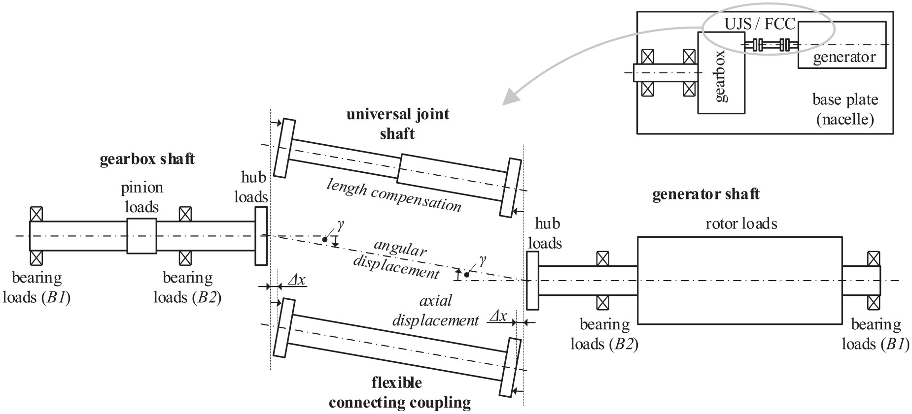
Gearbox and generator high speed shaft assembly.

FCCs use flexible elements between the shaft hubs to allow axial (Δx) and angular (γ) displacement. The flexible elements are realized by rubber or metal parts depending on the transmitted torque. Due to the high transmitted torque, FCCs applied in wind turbines use metal disk packs as flexible elements (cp. Figure 2 from Kang et al., 2016). The permissible magnitude of axial and angular displacement depends on the design of the coupling joint and metal disk pack itself determining the maximal allowable deformation and associated stresses of the metal disk pack. However, the deformation of the metal disk packs also causes reaction forces and moments which are transmitted to the primary and secondary side hubs of the coupling joint (cp. Figure 2) and thus to the gearbox and generator shafts (cp. Figure 1: hub loads).

Figure 2.

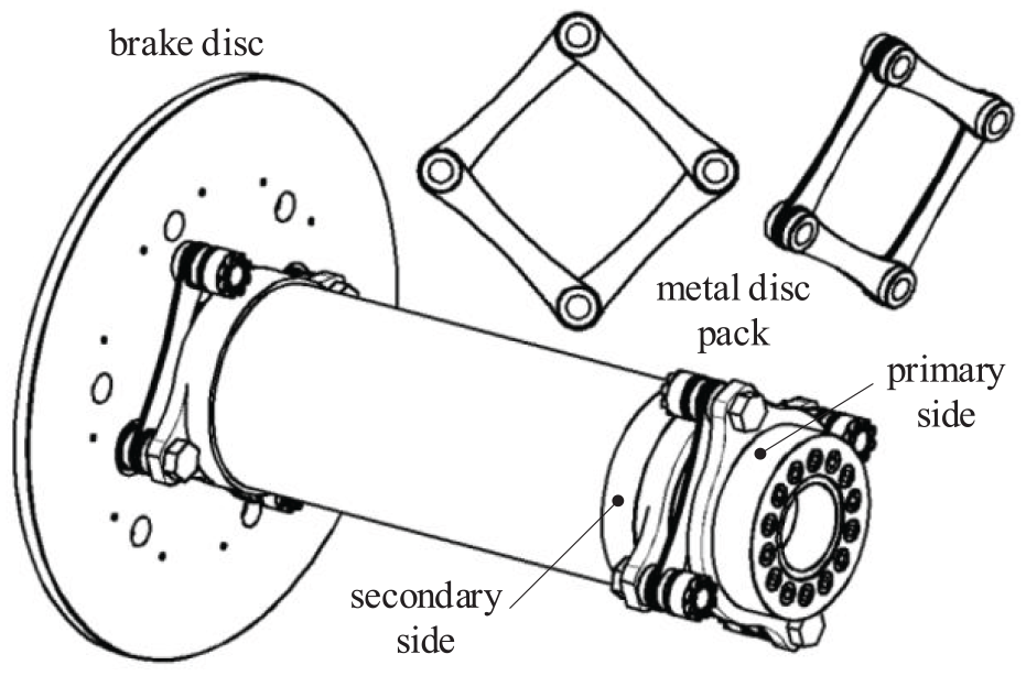
Design of flexible connecting coupling for wind turbines (Kang et al., 2016).

Furthermore, due to the joint kinematics of connecting couplings, additional loads are generated at the primary and secondary side hub. These loads are well known for a UJS; however, they also apply for FCCs. Therefore, the hub loads at the gearbox and generator shaft end are a combination of the loads due to the joint kinematics and those due to the deformation of metal disk packs (cp. also Figure 3). Both types of loads can be calculated by models describing the joint kinematics and disk pack deformation as a function of axial and angular displacement. These models are developed in section “Loads due to joint kinematics,” respectively, and in section “Loads due to disc pack deformations.” Then, from these models the reaction forces and moments (loads) can be evaluated at the connecting coupling hub (cp. Figure 3). By applying the reaction loads to a shaft-bearing assembly, the bearing loads are derived as will be shown in section “Bearing load calculation.” Finally, to quantify the hub reaction and bearing loads, axial and angular displacement during installation and operation are discussed and considered in section “Displacement estimation.”

Figure 3.

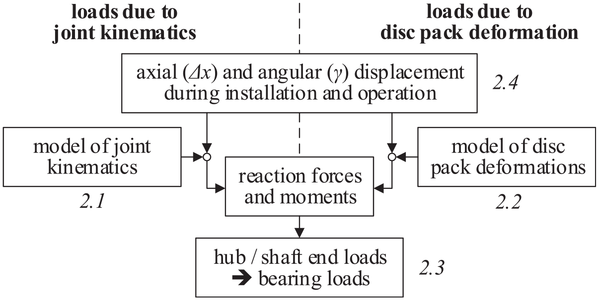
Process of load calculation.

Loads due to joint kinematics

It is well known that joints in UJSs and cardan shafts cause fluctuating shaft speeds, torques, and bending moments (Thoma, 1920). These quantities can be evaluated by considering the kinematic relation between the shaft speed before (ω₁) and after (ω₂) the joint (Thoma, 1920). This calculation makes use of the fact that a cross connection is present in the joints (cp. Figure 4a), that is, the rotating vectors e₁ and e₂ shown in Figure 4(a) and (b) are perpendicular (ψ = π/2). Therefore, their scalar product is equal to zero and a direct relation between the speeds ω₁ and ω₂ can be found (cp. Thoma (1920) for the principle of the derivation of equation (1))

$$\frac{{\omega }_2}{{\omega }_1}=\frac{\frac{\cos \beta }{\cos \alpha }}{[1+{(\tan \phi \frac{\cos \beta }{\cos \alpha }+\tan \alpha \sin \beta )}^2]{\cos }^2\phi }$$

(1)

Figure 4.

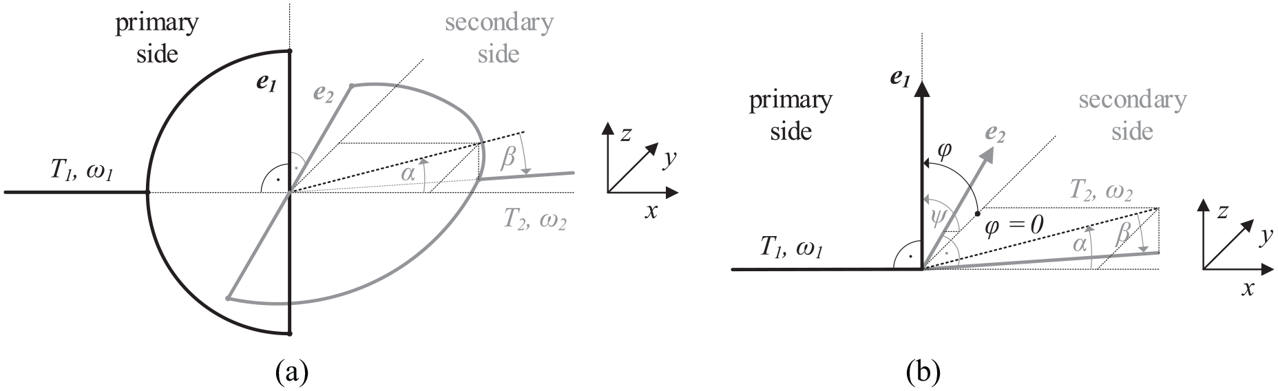
Primary and secondary side of coupling joint: a) cross connection ψ = π/2, and b) general connection.

This means that the speed ω₂ differs from the speed ω₁ depending on the displacement angles α and β and the shaft rotation (position) angle φ. The displacement angle α is the rotation of the secondary side around the z-coordinate and the displacement angle β to the rotation around the y-coordinate (cp. also Figure 4).

However, FCCs do not use a cross connection in the joint, that is, the angle ψ is not necessarily equal to π/2 (cp. Figure 5(a) to (c)). Hence, the scalar product of the two vectors e₁ and e₂ is not always zero anymore. Consequently, the kinematic relation between the speeds ω₁ and ω₂ cannot be evaluated in a straightforward manner as it is shown in Thoma (1920). An alternative method is needed to describe the kinematic relation between primary and secondary side. As the transmitted power, that is, the product of shaft speed ω and torque T, before and after the joint must be equal, the following relation is valid

$$\frac{{\omega }_2}{{\omega }_1}=\frac{T_1}{T_2}$$

(2)

Figure 5.

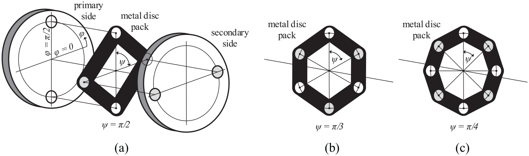
FCC joints with different angles ψ: (a) ψ = π/2, (b) ψ = π/3, and (c) ψ = π/4.

Therefore, the kinematic relation between the speeds ω₁ and ω₂ is equivalent to the relation of the torques T₁ and T₂. In other words, the kinematic relation after equation (1) can also be derived by evaluating the torques T₁ and T₂.

In addition, torque is the product of a radius and force. This means that for analyzing how the torque (T₂) is changed by the FCC joint with metal disk packs (Figure 5), the change of the radius R₂ and force F₂ must be described. It also means that by evaluating separately the change of radius R₂ and force F₂ and then by combining them, the kinematic relation in equation (1) can be found. To do so, a simplified pre-consideration of the kinematics is discussed before looking at the general consideration. The pre-consideration evaluates the kinematic loads at the rotating angle φ = 0 (change of radius) and φ = π/2 (change of force) for the displacement angle α ≠ 0, but β = 0. In a third case, the displacement angles are set to α = 0 and β ≠ 0. Note that the pre-considerations are valid for any angle ψ.

Pre-consideration

As a first case, the FCC joint is schematically shown in Figure 6 for a rotation angle φ = 0, which represents the change of radius case. Primary and secondary sides have an angular displacement (i.e. misalignment) given by the angle α, that is, the secondary side rotates by the angle α around the z-axis. Due to this rotation, the effective radius which transmits the force from the primary to the secondary side reduces from R to R_y (cp. Figure 6). As a consequence of this, the transmitted force should increase from F₁ to F₂ because the torque of the primary side is constant.

Figure 6.

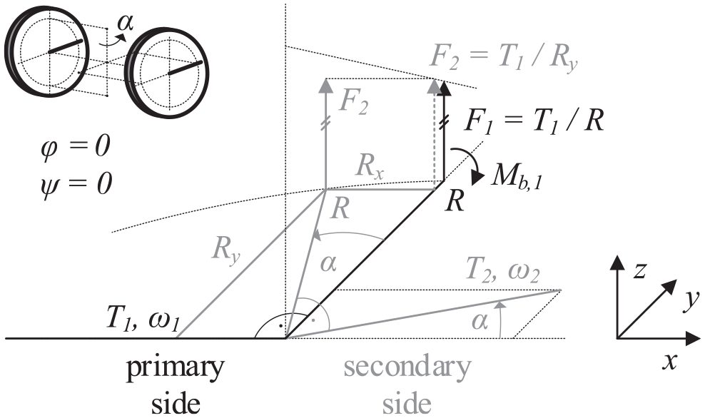
Pre-consideration case 1, change of radius: φ = 0 and β = 0.

Furthermore, because of the rotation around the z-axis, the working lines of force F₁ and F₂ are still parallel; however, they do not coincide anymore, that is, they are separated by the distance R_x. This means that a bending moment (M_b,₁) is introduced to the primary side in order to transmit the force from the primary to the secondary side. Then, the torque T₂ of the secondary side is the product of the increased transmitted force F₂ and the radius R. So the equations valid for the connecting coupling position shown in Figure 6 are given as follows

$$T_1=F_{1}R$$

(3)

$$F_2=T_1/R_y=F_{1}R/R_y=F_{1}1/A_{R,\alpha y}$$

(4)

$$T_2=F_{2}R=T_1/A_{R,\alpha y}$$

(5)

$$M_{b,1}=-F_2{R}_x=-F_1{R}_x/A_{R,\alpha y}=T_1{A}_{R\alpha ,x}/A_{R,\alpha y}=T_1{A}_{B1,\alpha }$$

(6)

where A_R,α is the radius transfer function describing the modification of torque T₂ due to angle α. The bending transfer function (at the primary side) due to angle α is indicated by A_B1,α. With Figure 6, these transfer functions can be extended to be valid for any value of the rotating angle φ by

$$A_{R,\alpha y}=R_y/R=\sqrt{{\left(\cos \alpha \cos \phi \right)}^2+{\left(\sin \phi \right)}^2}$$

(7)

$$A_{R,\alpha x}=R_x/R=-\sin \alpha \sqrt{{\left(\cos \phi \right)}^2}=-\mathrm{sgn}\alpha \sqrt{{\left(\sin \alpha \cos \phi \right)}^2}$$

(8)

$$A_{B1,\alpha }=A_{R,\alpha x}/A_{R,\alpha y}=-\mathrm{sgn}\alpha \sqrt{\frac{{\left(\sin \alpha \cos \phi \right)}^2}{{\left(\cos \alpha \cos \phi \right)}^2+{\left(\sin \phi \right)}^2}}$$

(9)

In the second case, the FCC joint visible in Figure 6 is rotated by an angle φ = π/2. This leads to the joint position as shown in Figure 7, which represent the change of force case.

Figure 7.

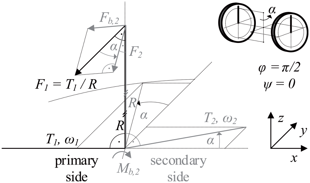
Pre-consideration case 2, change of force: φ = π/2 and β = 0.

It can be seen from Figure 7 that due to the rotation of φ = π/2, the radii of the primary and secondary side coincide, as the misalignment (angle α) is in the xy-plane. This, however, means that the working lines of force F₁ and F₂ deviate with the displacement angle α (change of force). Consequently, the force F₁ of the primary side is upon transmission split into a force F₂ and F_b,₂. The force F₂ generates (with the radius R) the torsional torque T₂ of the secondary side, while the force F_b,₂ creates (with the radius R) the bending moment M_b,₂ at the secondary side. The equations valid for the FCC joint position shown in Figure 7 are given as follows

$$F_2=F_1·A_{F,\alpha }$$

(10)

$$F_{b,2}=F_1·A_{B2,\alpha }$$

(11)

$$T_2=F_{2}R=T_1·A_{F,\alpha }$$

(12)

$$M_{b,2}=-F_{b,2}R=T_1·A_{B2,\alpha }$$

(13)

with A_F,α the force transfer function and A_B2,α the bending transfer function (at the secondary side) due to angle α. Based on Figure 7, the transfer functions are generalized again and can be specified as a function of the rotating angle φ by

$$A_{F,\alpha }=F_2/F_1=\sqrt{{\left(\cos \alpha \sin \phi \right)}^2+{\left(\cos \phi \right)}^2}$$

(14)

$$A_{B2,\alpha }=F_{b,2}/F_1=-\sin \alpha \sqrt{{\left(\sin \phi \right)}^2}=-\mathrm{sgn}\alpha \sqrt{{\left(\sin \alpha \sin \phi \right)}^2}$$

(15)

It can be seen that the secondary side torque T₂ can be modified by the transfer functions in both equation (7) (due to a change in effective radius) and equation (14) (change in force). So these two equations must be combined to obtain the total torque transfer function. From equation (5), it is visible that the primary torque is divided by A_R,αy and from equation (12) that the primary torque is multiplied by A_F,α. This means that the torque transfer function A_T,α for a displacement angle α (and any rotation angle φ) is A_F,α divided by A_R,αy, that is

$$A_{T,\alpha }=T_2/T_1=A_{F,\alpha }/A_{R,\alpha y}=\sqrt{\frac{{\left(\cos \alpha \sin \phi \right)}^2+{\left(\cos \phi \right)}^2}{{\left(\cos \alpha \cos \phi \right)}^2+{\left(\sin \phi \right)}^2}}$$

(16)

And finally, as a third case, in the same way as shown for the displacement angle α, the torque and bending transfer functions can be obtained for the displacement angle β ≠ 0, but α = 0. Considering that the displacement angle β is equivalent to a phase shift of −π/2 in comparison with the displacement angle α (cp. Figure 4(b)), the transfer functions are obtained as follows

$$A_{T,\beta }=\sqrt{\frac{{\left(\cos \beta \cos \phi \right)}^2+{\left(\sin \phi \right)}^2}{{\left(\cos \beta \sin \phi \right)}^2+{\left(\cos \phi \right)}^2}}$$

(17)

$$A_{B1,\beta }=\mathrm{sgn}\beta \sqrt{\frac{{\left(\sin \beta \sin \phi \right)}^2}{{\left(\cos \beta \sin \phi \right)}^2+{\left(\cos \phi \right)}^2}}$$

(18)

$$A_{B2,\beta }=\mathrm{sgn}\beta \sqrt{{\left(\sin \beta \cos \phi \right)}^2}$$

(19)

The pre-consideration of the FCC joint demonstrates that the torque of the secondary side as well as the bending moments of the primary and secondary side can be expressed as functions of the torque of the primary side, if the displacement angles and thus the transfer functions are known. Therefore, in the following general consideration, the radius and force transfer functions are derived taking into account the angles φ, ψ, α, β (cp. also Figure 4(b)).

General consideration

The alpha (equations (9), (15), and (16)) and beta (equations (17) to (19)) transfer functions are particular forms of the general transfer functions. This means that the general transfer functions can be derived from them. If the displacement angles α ≠ 0 and β ≠ 0, then an equivalent displacement angle γ will be calculated by (see also Figure 8(a) in combination with Table 1)

$$\gamma =\mathrm{sgn}\left(\alpha \right)\arccos \left(\cos \alpha \cos \beta \right)$$

(20)

Figure 8.

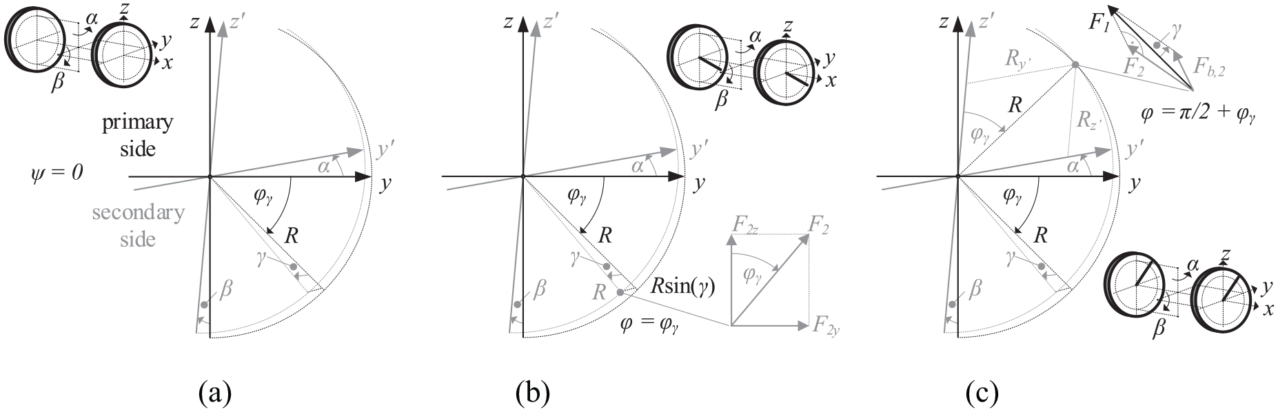
(a) Displacement angle γ and phase angle φ_γ due to the combination of α and β; (b) reaction forces due to angle γ and at rotation angle φ = φ_γ (change of radius); and (c) reaction forces due to angle γ and at rotation angle φ = π/2 + φ_γ (change of force).

Table 1.

Displacement angle γ and phase angle φ_γ dependent on angles α and β.

Angle α	Angle β	Angle γ	Angle φγ
>0	0	α	–0
>0	>0	>0	<0
>0	<0	<0	>0
<0	0	A	+0
<0	>0	>0	>0
<0	<0	<0	<0
+0	>0	β	–π/2
+0	<0	β	π/2

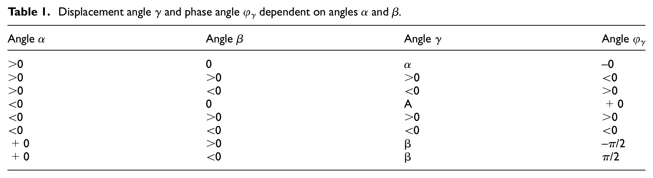
Furthermore, the position of the equivalent displacement angle is specified by the phase angle φ_γ (cp. Figure 8(a)), which can be derived from the displacement angles α and β (cp. Figure 8(a) and Table 1) as

$$\tan {\phi }_{\gamma }=-\frac{\beta }{\alpha }$$

(21)

At the position φ = φ_γ, the reaction forces are parallel to the yz-plane and thus can be decomposed in a force component in y- and z-direction. This is shown in Figure 8(b) which is equivalent to the pre-consideration case 1, change of radius in Figure 6. It also means that the primary side shaft bending has components around y- and z- direction (cp. Figure 8(b)).

Then, at the position φ = π/2+φ_γ, the secondary side is in plane with the primary side, that is, the radii of primary and secondary side coincide. This is demonstrated in Figure 8(c) which is equivalent to the pre-consideration case 2, change of force in Figure 7. At this position, the working lines of the reaction forces cross. The reaction force F_b,₂, which is parallel to the rotating axis of the secondary side (x′-axis) and normal to the rotated y′z′-plane causes shaft bending of the secondary side (cp. Figure 8(c)). This shaft bending can, again, be split in its components because the secondary side radius can be decomposed, too.

Based on these considerations, the radius A_R,γ (cp. Figure 8(b)) and force A_F,γ (cp. Figure 8(c)) transfer functions can be derived for the equivalent displacement angle γ. By, again, combining the radius A_R,γ and force A_F,γ transfer functions, the torque transfer function is obtained. The detailed derivations of the radius (A_R,γ) and force (A_F,γ) transfer functions are not shown here for space limitation reasons. The resulting torque (A_T,γ) and bending transfer functions (A_B1,γ and A_B2,γ) are

$$A_{T,\gamma }=A_{F,\gamma }/A_{R,\gamma y}=\sqrt{\frac{{\left(\cos \gamma \sin (\phi -\psi -{\phi }_{\gamma })\right)}^2+{\left(\cos (\phi -\psi -{\phi }_{\gamma })\right)}^2}{{\left(\cos \gamma \cos (\phi -\psi -{\phi }_{\gamma })\right)}^2+{\left(\sin (\phi -\psi -{\phi }_{\gamma })\right)}^2}}$$

(22)

$$A_{B1,\gamma }=-\mathrm{sgn}\gamma \sqrt{\frac{{\left(\sin \gamma \cos (\phi -\psi -{\phi }_{\gamma })\right)}^2}{{\left(\cos \gamma \cos (\phi -\psi -{\phi }_{\gamma })\right)}^2+{\left(\sin (\phi -\psi -{\phi }_{\gamma })\right)}^2}}\left(\begin{array}{c}0\hfill \\ \multicolumn{1}{c}{\cos {\phi }_{\gamma }}\\ \multicolumn{1}{c}{\sin {\phi }_{\gamma }}\end{array}\right)$$

(23)

$$A_{B2,\gamma }=-\mathrm{sgn}\gamma \sqrt{{\left(\sin \gamma \sin (\phi -\psi -{\phi }_{\gamma })\right)}^2}\left(\begin{array}{c}0\hfill \\ \multicolumn{1}{c}{\cos {\phi }_{\gamma }}\\ \multicolumn{1}{c}{\sin {\phi }_{\gamma }}\end{array}\right)$$

(24)

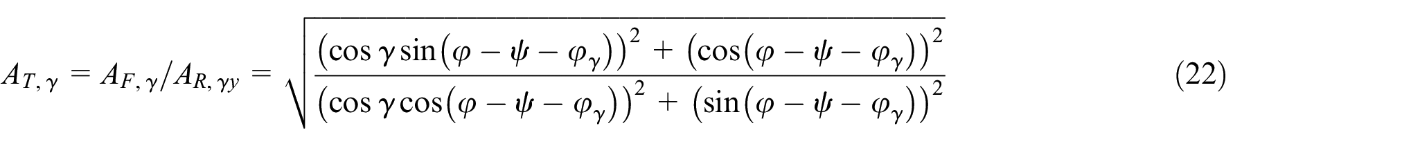
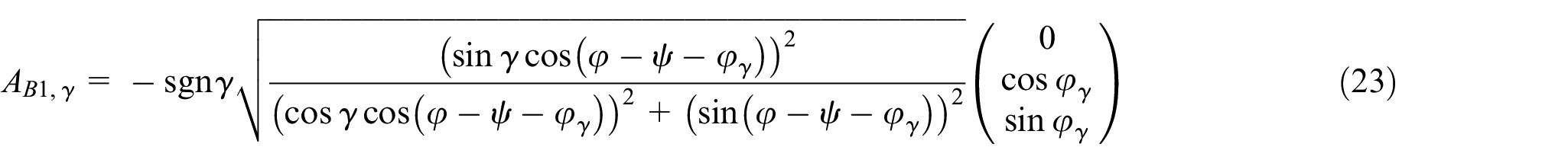
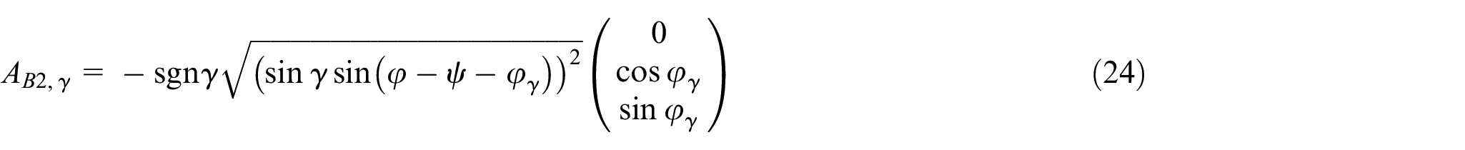
Note that the general torque and bending transfer functions in equations (22)–(24) are valid for every connection between primary and secondary side. The vector in equation (23) is needed to split the bending moment in its components around y- and z-direction. The same applies for equation (24), that is, the vector splits the bending moment in its components around y′- and z′-direction

Moreover, note that the number of connections n is defined by the design of the FCC joint. For example, FCCs shown in Figure 5(a) to (c) have each two, three, and four connections, respectively, at primary and secondary side. This means that the angle ψ is related to the number of connections n as

$$\psi =\frac{\pi }{n}$$

(25)

To evaluate the transfer functions of the FCC joint, equations (22)–(24) must be calculated for every connection (of the secondary side). It can be assumed that each of the n connections transmits the nth part of the primary side torque. So the transfer functions of the connecting coupling are obtained by summing up the torques and bending moments of the n connections, that is

$$T_2=\sum _{i=1}^n\frac{T_1}{n}{A}_{T,\gamma ,i}$$

(26)

$$M_{b,1}=\sum _{i=1}^n\frac{T_1}{n}{A}_{B1,\gamma ,i}$$

(27)

$$M_{b,2}=\sum _{i=1}^n\frac{T_1}{n}{A}_{B2,\gamma ,i}$$

(28)

Note that in the case of n = 2 connections, the transfer functions for i = 1 and i = 2 are identical. This means that in this case a summation after equations (26)–(28) is not necessary and the torque and bending moments can be directly determined from the transfer functions. In the pre-considerations, this simplification was utilized.

Furthermore, from equations (26)–(28, it can be seen that torque fluctuations and shaft bending moments occur at any type of FCC joint using n connections at primary and secondary side. Moreover, according to equation (2), the inverse of the torque ratio in equation (22) for n = 2 connections, that is, ψ = π/2, must be equivalent to equation (1). Remember that equation (1) describes the kinematic relation of the primary and secondary shaft speed with a cross connection (ψ = π/2) in the joint. Figure 9 shows this comparison for one shaft rotation, demonstrating that equations (1) and (22) are indeed equivalent. In addition, equation (27) provides the bending moment components around the y- and z-axes and equation (28) provides the bending moment components around the y′- and z′-axes because equations (23) and (24) include a vector decomposition. This is needed for the hub/bearing load calculations in y- and z-direction. Therefore, it can be concluded that the loads due to the kinematics of the coupling joint (cp. also Figure 3) can be calculated by equations (22)–(24), respectively, and equations (26)–(28).

Figure 9.

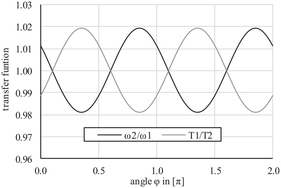
Comparison of transfer functions for α = 5° and β = 10°.

Figure 10 shows the absolute value of the primary side bending moment for connecting couplings with n = 2, n = 3, and n = 4 connections over one shaft rotation. For n = 3 and n = 4, the superposition of different connections can be observed since the fluctuation (amplitude) of the bending moment reduces significantly. This demonstrates that the bending moment (over one rotation) converges to an almost constant value by increasing the number of connections at primary and secondary side. So the primary (M_b,₁) and secondary (M_b,₂) side bending moments of FCCs with a higher number of connections can be considered as constant in time. Note that this also applies to the secondary side torque (T₂) for even-numbered connections, that is, nϵ {4, 6, 8, …}, as can be derived from equation (24).

Figure 10.

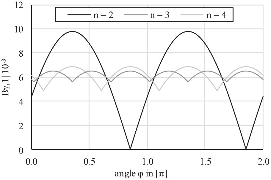
Bending of primary side shaft for α = 0.5° and β = 0.25°.

Although the joint kinematics do not generate any axial forces, in the case of UJSs with length compensation axial forces occur which must be absorbed by the primary side shaft bearings. These axial forces are caused by the transmitted torque and friction between the flanks of the profiles while compensating the axial length (Elbe-Group, n.d.; Voith, 2015). the primary side torque T₁, the profile pitch diameter D _p , friction coefficient μ _f as well as displacement angles, α and β, the (maximal) reaction force at the primary side due to length compensation can be calculated as follows (Elbe-Group, 2014; Voith, 2015)

$${\overrightarrow{F}}_{\max }=\left(\begin{array}{c}{F}_x\hfill \\ \multicolumn{1}{c}{F_y}\\ \multicolumn{1}{c}{F_z}\end{array}\right)={\mu }_f{T}_1\frac{2}{D_p}\left(\begin{array}{c}1\hfill \\ \multicolumn{1}{c}{\tan \gamma \cos {\phi }_{\gamma }}\\ \multicolumn{1}{c}{\tan \gamma \sin {\phi }_{\gamma }}\end{array}\right)$$

(29)

Note that the axial forces and thus also the forces in equation (29) slightly increase due to the pressure built up in the length compensation during lubrication (Voith, 2015). This effect, however, is neglected in this article.

To summarize, the kinematics of the joints result in variations (over shaft position or time) of rotational speed and transmitted torque. The equations derived in this subsection enable to quantify these variations for any misalignment angle and joint design (number of connections). Moreover, bending moments are generated in both the primary and secondary sides of the joints. Also these moments can be quantified using the proposed equations. In the next subsection, the second type of loads generated in joints will be discussed in detail.

Loads due to disk pack deformations

As already mentioned above, metal disk packs are commonly used in FCC joints which have to transmit high torques. The metal disk packs provide, on the one hand, a high torsional stiffness and allow, on the other hand, axial and angular shaft misalignment. This means that the metal disks have a high tension/compression stiffness and simultaneously a low bending and twist stiffness. Consequently, it can be assumed that the reaction loads, that is, the forces that the coupling exerts on the two connected shafts, due to disk pack deformations are dominated by the tension/compression stiffness. Therefore, for the reaction load calculation, the metal disk packs can be approximated by a set of 1D springs which have a tension/compression stiffness k_1D (cp. Figure 11).

Figure 11.

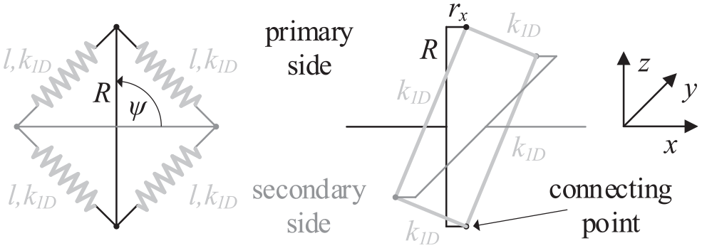
Representation of an FCC joint with ψ = π/2 by a set of 1D springs: front view (left) and 3D sketch (right).

The stiffness k_1D can be evaluated from the torsional stiffness k_t of the metal disk pack which is normally given in the FCC data sheet. For an FCC with each two (spring) connecting points at primary and secondary side (cp. Figure 11), that is, ψ = π/2, the spring force due to the transmitted torque T₁ is given as

$$F_{\mathrm{spring}}=\frac{T_1}{2R}\sin \left(\frac{\psi }{2}\right)=\frac{T_1}{2\sqrt{2}R}=k_{1D}\mathrm{\Delta }l=k_{1D}2R[\sin \left(\frac{\psi +\mathrm{\Delta }\psi }{2}\right)-\sin \left(\frac{\psi }{2}\right)]$$

(30)

The spring extension Δl is specified by the difference between the deformed (l′) and undeformed (l) length of the 1D spring. In addition, for small angles Δψ and for ψ = π/2, equation (30) can be simplified by using

$$\sin \left(\frac{\psi +\mathrm{\Delta }\psi }{2}\right)-\sin \left(\frac{\psi }{2}\right)=\sin \left(\frac{\psi }{2}\right)\cos \left(\frac{\mathrm{\Delta }\psi }{2}\right)+\cos \left(\frac{\psi }{2}\right)\sin \left(\frac{\mathrm{\Delta }\psi }{2}\right)-\sin \left(\frac{\psi }{2}\right)=\frac{\mathrm{\Delta }\psi }{2\sqrt{2}}$$

(31)

Then, with the torsional stiffness k_t specified by the quotient of the torque T₁ and torsional displacement angle Δψ, the stiffness k_1D can be written as follows

$$k_{1D}=\frac{F_{\mathrm{spring}}}{\mathrm{\Delta }l}=\frac{T_1}{2\sqrt{2}R}\frac{2\sqrt{2}}{2R\mathrm{\Delta }\psi }=\frac{1}{2R^2}\frac{T_1}{\mathrm{\Delta }\psi }=\frac{1}{2R^2}{k}_t$$

(32)

Hence, based on the product of the spring stiffness k_1D and the spring extension Δl due to angular (γ) and axial (Δx) displacement, the reaction forces and moments can be calculated at the shaft centers of the primary and secondary side. As the forces and moments are equal at the primary and secondary side, it is sufficient to calculate them at the primary side. The spring extension due to axial (Δl_Δx) and angular (Δl_γ) displacement is evaluated based on Figure 12. It is for small angles

$$\mathrm{\Delta }{l}_{\mathrm{\Delta }x}=l\prime -l=\sqrt{l^2+\mathrm{\Delta }{x}^2}-l=\sqrt{2}R(\sqrt{1+{\left(\frac{\mathrm{\Delta }x}{l}\right)}^2}-1)\approx \sqrt{2}R(\sqrt{1+{\left(\tan \frac{\delta }{\sqrt{2}}\right)}^2}-1)$$

(33)

$$\mathrm{\Delta }{l}_{\gamma }=l\prime -l\approx \sqrt{2}R(\sqrt{1+{\left(\tan \frac{\gamma }{\sqrt{2}}\right)}^2}-1)$$

(34)

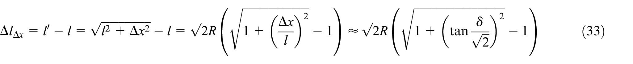
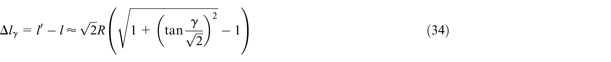
Equations (33) and (34) can be simplified by the following trigonometric relation

$$\sqrt{1+{\left(\tan \gamma \right)}^2}=\frac{1}{\cos \gamma }$$

(35)

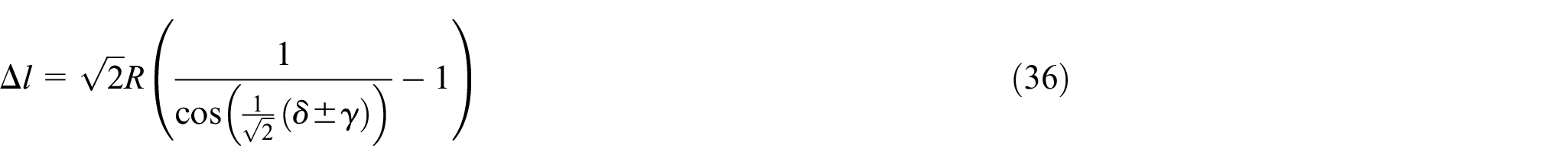
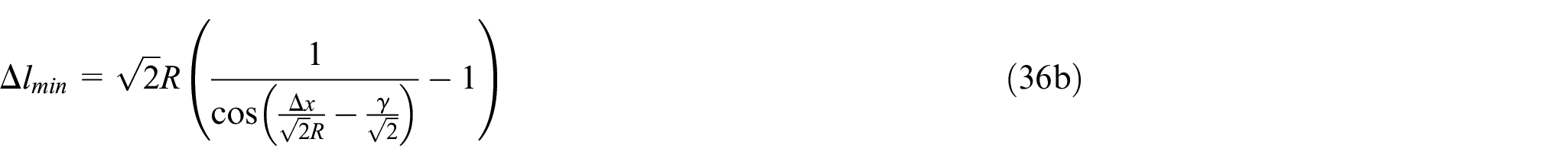
Then, the total spring extension due to angular (γ) and axial (Δx) displacement is approximated for small angles by (cp. Figure 12)

$$\mathrm{\Delta }l=\sqrt{2}R(\frac{1}{\cos \left(\frac{1}{\sqrt{2}}(\delta \pm \gamma )\right)}-1)$$

(36)

Figure 12.

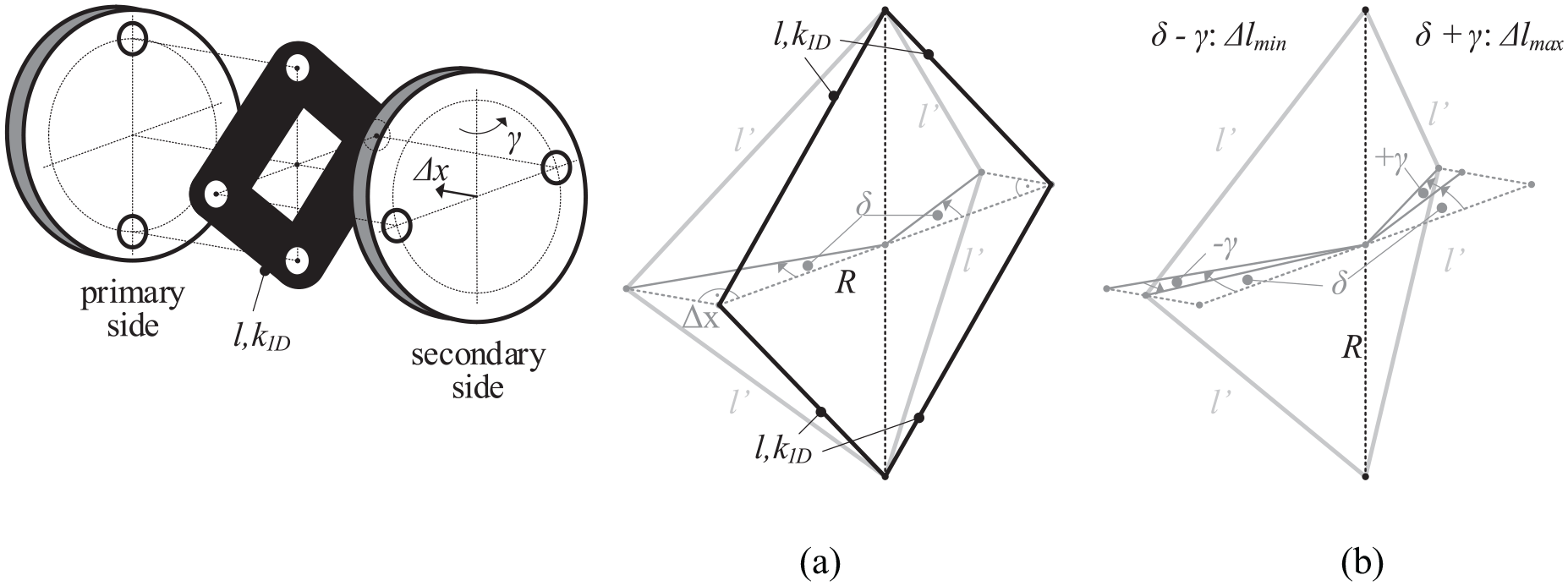
Tensioning of 1D springs due to displacement: (a) axial Δx and (b) combination of axial Δx and angular γ.

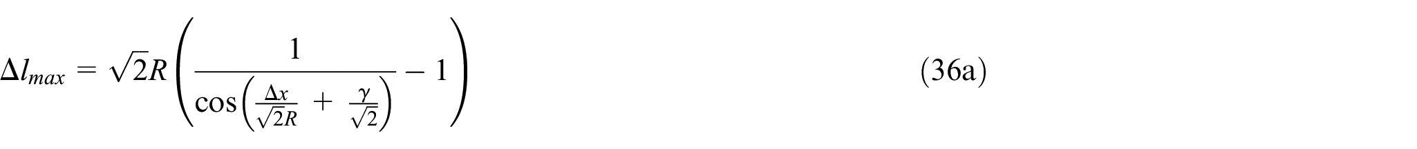
Note that due to the combination of angular and axial displacement, the extension is not equal for the different springs. In other words, one half of the springs is tensioned until Δl_max, while the other half of the springs only until Δl_min

$$\mathrm{\Delta }{l}_{\max }=\sqrt{2}R(\frac{1}{\cos (\frac{\mathrm{\Delta }x}{\sqrt{2}R}+\frac{\gamma }{\sqrt{2}})}-1)$$

(36a)

$$\mathrm{\Delta }{l}_{\min }=\sqrt{2}R(\frac{1}{\cos (\frac{\mathrm{\Delta }x}{\sqrt{2}R}-\frac{\gamma }{\sqrt{2}})}-1)$$

(36b)

Furthermore, due the unequal extension, the spring forces at the connecting points are neither equal, that is, a force difference occurs at the spring connecting points. This means that reaction forces (vector F) and moments (vector M_b) appear at the shaft center. These forces and moments are specified based on Figure 13 as follows

$$F_{\max }=k_{1D}\mathrm{\Delta }{l}_{\max }$$

(37a)

$$F_{\min }=k_{1D}\mathrm{\Delta }{l}_{\min }$$

(37b)

$$F_{\mathrm{axial}}=2[F_{\min }\sin (\frac{\mathrm{\Delta }x}{\sqrt{2}R}-\frac{\gamma }{\sqrt{2}})+F_{\max }\sin (\frac{\mathrm{\Delta }x}{\sqrt{2}R}+\frac{\gamma }{\sqrt{2}})]$$

(38)

$$F_{\mathrm{radial}}=2\sin \left(\frac{\psi }{2}\right)[F_{\min }\cos (\frac{\mathrm{\Delta }x}{\sqrt{2}R}-\frac{\gamma }{\sqrt{2}})-F_{\max }\cos (\frac{\mathrm{\Delta }x}{\sqrt{2}R}+\frac{\gamma }{\sqrt{2}})]$$

(39)

$$\overrightarrow{F}=\left(\begin{array}{c}{F}_x\hfill \\ \multicolumn{1}{c}{F_y}\\ \multicolumn{1}{c}{F_z}\end{array}\right)=\left(\begin{array}{c}{F}_{\mathrm{axial}}\hfill \\ \multicolumn{1}{c}{F_{\mathrm{radial}}\cos {\psi }_{\gamma }}\\ \multicolumn{1}{c}{F_{\mathrm{radial}}\sin {\psi }_{\gamma }}\end{array}\right)$$

(40)

$${\overrightarrow{M}}_b=\left(\begin{array}{c}0\hfill \\ \multicolumn{1}{c}{M_{b,y}}\\ \multicolumn{1}{c}{M_{b,z}}\end{array}\right)=\left(\begin{array}{c}{r}_x\hfill \\ \multicolumn{1}{c}{0}\\ \multicolumn{1}{c}{0}\end{array}\right)\times \left(\begin{array}{c}{F}_x\hfill \\ \multicolumn{1}{c}{F_y}\\ \multicolumn{1}{c}{F_z}\end{array}\right)=\left(\begin{array}{c}0\hfill \\ \multicolumn{1}{c}{-r_x{F}_z}\\ \multicolumn{1}{c}{r_x{F}_y}\end{array}\right)$$

(41)

Figure 13.

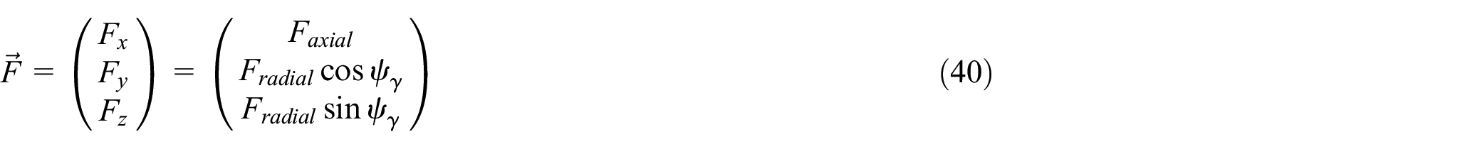
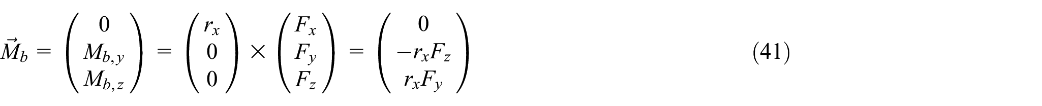
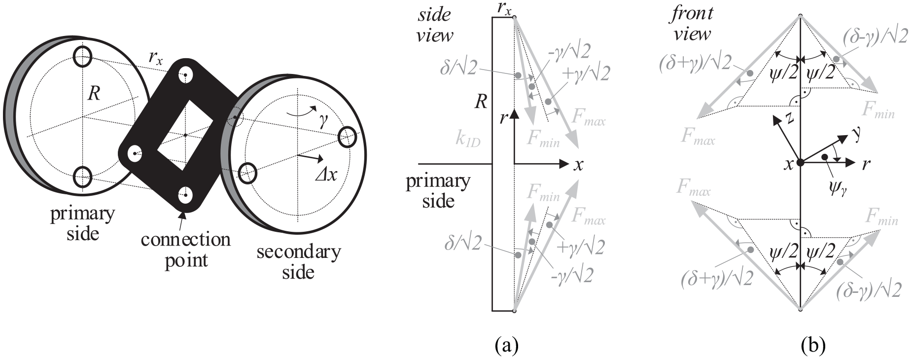
Minimal and maximal forces at spring (disk pack) connection points of primary side caused by axial (Δx) and angular (γ) displacement: (a) side view and (b) front view seen from secondary side.

To summarize, it can be seen from equations (36) to (39) that the hub loads (equations (40) and (41)) at the gearbox and generator shaft end (cp. also Figure 1) caused by disk pack deformations can be calculated from the torsional disk pack stiffness (k_t) and by given axial (Δx) and angular (γ) displacements. It is important to note that, because of approximating the metal disk packs with 1D tension/compression springs, the calculated reaction loads are lower than the loads which occur in reality, that is, the load calculation is non-conservative. Nevertheless, the calculated reaction loads are a proper approximation of the real loads because with the torsional stiffness the dominate disk pack stiffness is considered. It should be recalled that the metal disk packs are designed to transmit high torques (=high torsional stiffness of disk packs) and to allow simultaneously axial and angular misalignment (=low bending and twisting stiffness of disk packs).

Bearing load calculation

After evaluating the (hub) loads due to joint kinematics and disk pack deformation, the bearing loads are considered. To analyze the effect of axial and angular displacement on gearbox and generator shaft bearings, it is sufficient to have a closer look at one of these shafts (cp. also Figure 1). As a shorter bearing spacing increases the bearing loads and the gearbox shaft is normally shorter than the generator shaft, the gearbox shaft is considered to be more critical and thus, is analyzed in this article. In the bearing load calculation of the gearbox shaft (cp. Figure 14), the following loads are taken into account: the shaft weight G_S, (radial) forces of the (spur-toothed) pinion F_P, the reaction force F_H, and moment M_H at the shaft end (hub) due to the joint kinematics and metal disk pack deformation as well as the half weight G_H of the FCC (or UJS). The length l_B is the distance between bearing B1 and B2, l_P is the distance between the pinion and bearing B2, and l_H is the distance between bearing B2 and hub.

Figure 14.

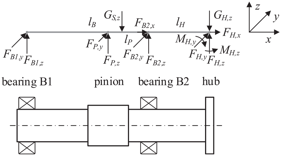
Forces and moments acting on a shaft with pinion and hub.

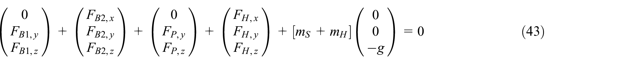
Furthermore, bearing loads are often calculated based on static force and moment balance considerations and can be evaluated by taking the sum of all forces and moments acting on the shaft and equating this sum to zero (force balance). So for the shaft assembly shown in Figure 14, the bearing forces are calculated as follows

$$\begin{array}{c}\underset{¯}{\mathrm{\Sigma }F:}\hfill \\ {\overrightarrow{F}}_{B1}+{\overrightarrow{F}}_{B2}+{\overrightarrow{F}}_P+{\overrightarrow{F}}_H+{\overrightarrow{G}}_S+{\overrightarrow{G}}_H=0\hfill \end{array}$$

(42)

$$\left(\begin{array}{c}0\hfill \\ \multicolumn{1}{c}{F_{B1,y}}\\ \multicolumn{1}{c}{F_{B1,z}}\end{array}\right)+\left(\begin{array}{c}{F}_{B2,x}\hfill \\ \multicolumn{1}{c}{F_{B2,y}}\\ \multicolumn{1}{c}{F_{B2,z}}\end{array}\right)+\left(\begin{array}{c}0\hfill \\ \multicolumn{1}{c}{F_{P,y}}\\ \multicolumn{1}{c}{F_{P,z}}\end{array}\right)+\left(\begin{array}{c}{F}_{H,x}\hfill \\ \multicolumn{1}{c}{F_{H,y}}\\ \multicolumn{1}{c}{F_{H,z}}\end{array}\right)+[m_S+m_H]\left(\begin{array}{c}0\hfill \\ \multicolumn{1}{c}{0}\\ \multicolumn{1}{c}{-g}\end{array}\right)=0$$

(43)

and similar for the momentum balance

$$\begin{array}{c}\underset{¯}{\mathrm{\Sigma }M:}\hfill \\ {\overrightarrow{M}}_H+{\overrightarrow{l}}_{B1}\times {\overrightarrow{F}}_{B1}+{\overrightarrow{l}}_{B2}\times {\overrightarrow{F}}_{B2}+{\overrightarrow{l}}_P\times {\overrightarrow{F}}_P+{\overrightarrow{l}}_S\times {\overrightarrow{G}}_S=0\hfill \end{array}$$

(44)

$$\left(\begin{array}{c}0\hfill \\ \multicolumn{1}{c}{M_{H,y}}\\ \multicolumn{1}{c}{-M_{H,z}}\end{array}\right)+\left(\begin{array}{c}{l}_B+l_H\hfill \\ \multicolumn{1}{c}{0}\\ \multicolumn{1}{c}{0}\end{array}\right)\times \left(\begin{array}{c}0\hfill \\ \multicolumn{1}{c}{F_{B1,y}}\\ \multicolumn{1}{c}{F_{B1,z}}\end{array}\right)+\left(\begin{array}{c}{l}_H\hfill \\ \multicolumn{1}{c}{0}\\ \multicolumn{1}{c}{0}\end{array}\right)\times \left(\begin{array}{c}{F}_{B2,x}\hfill \\ \multicolumn{1}{c}{F_{B2,y}}\\ \multicolumn{1}{c}{F_{B2,z}}\end{array}\right)+\left(\begin{array}{c}{l}_p+l_H\hfill \\ \multicolumn{1}{c}{0}\\ \multicolumn{1}{c}{0}\end{array}\right)\times \left(\begin{array}{c}0\hfill \\ \multicolumn{1}{c}{F_{P,y}}\\ \multicolumn{1}{c}{F_{P,z}}\end{array}\right)+\frac{m_S}{2}\left(\begin{array}{c}{l}_B+l_H\hfill \\ \multicolumn{1}{c}{0}\\ \multicolumn{1}{c}{0}\end{array}\right)\times \left(\begin{array}{c}0\hfill \\ \multicolumn{1}{c}{0}\\ \multicolumn{1}{c}{-g}\end{array}\right)=0$$

(45)

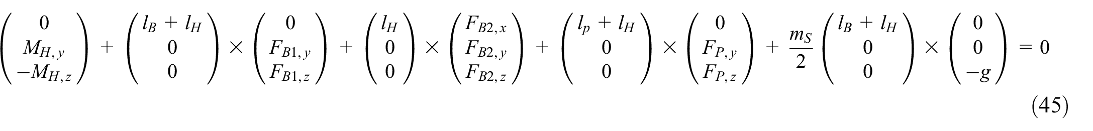
Note that pinions are normally designed as small as possible, that is, the pinion and shaft diameter are almost equal. Therefore, the pinion weight is neglected in equations (42) to (45) and only the shaft and hub weights are considered. By solving the system of equations in equations (43) and (45), the bearing forces F_B1 and F_B2 are obtained

$$F_{B1,y}=\frac{1}{l_B}{M}_{H,z}-\frac{l_P}{l_B}{F}_{P,y}+\frac{l_H}{l_B}{F}_{H,y}$$

(46)

$$F_{B1,z}=-\frac{1}{l_B}{M}_{H,y}-\frac{l_P}{l_B}{F}_{P,z}+\frac{l_H}{l_B}{F}_{H,z}+g[\frac{m_S}{2}(1-\frac{l_H}{l_B})-m_H\frac{l_H}{l_B}]$$

(47)

$$F_{B2,x}=-F_{H,x}$$

(48)

$$F_{B2,y}=-[\frac{1}{l_B}{M}_{H,z}+(1-\frac{l_P}{l_B})F_{P,y}+(1+\frac{l_H}{l_B})F_{H,y}]$$

(49)

$$F_{B2,z}=\frac{1}{l_B}{M}_{H,y}-(1-\frac{l_P}{l_B})F_{P,z}-(1+\frac{l_H}{l_B})F_{H,z}-g[\frac{m_S}{2}\frac{{(l_B+l_H)}^2}{l_B{l}_H}-m_H(1+\frac{l_H}{l_B})]$$

(50)

The hub forces F_H in x-, y- and z-direction and moments M_H around y- and z-axis are caused by the joint kinematics and metal disk pack deformations due to angular and axial displacement (cp. previous sections). The pinion force can be evaluated by the transmitted torque and pinion diameter D_p (approx. shaft diameter D_S)

$$F_{P,y}=\frac{2T_1}{D_P}\tan \theta$$

(51)

$$F_{P,z}=\frac{2T_1}{D_P}$$

(52)

Therefore, the bearing loads in equations (46) to (50) can be derived from shaft displacement (axial Δx and angular γ), torsional metal disk pack stiffness (k_t), and transmitted torque (T₁).

In addition, the presented bearing load calculation considering the hub loads due to coupling joint kinematics and disk pack deformation will be applied to an FCC and UJS in section “Performance of flexible connecting couplings.” To execute the calculation, the hub gravity force G_Hz (in Figure 14) has to be evaluated. Due to missing detailed information of the geometry and material of FCC and UJS, the weight of FCC and UJS is estimated (in this article) by hollow and solid shafts (cylinder), respectively, as follows:

• Shaft weight with pinion, estimated by a solid cylinder

$$m_S={\rho }_{\mathrm{steel}}{V}_S={\rho }_{\mathrm{steel}}\frac{\pi }{4}{D}_S^2(l_B+l_H)$$

(53)

• Hub weight due to half flexible coupling weight (cp. also FCC shown in Figure 2 and Kang et al., 2016)

$$m_{H,\mathrm{FCC}}={\rho }_{\mathrm{steel}}{V}_{\mathrm{FCC},1}+{\rho }_{\mathrm{GFRP}}{V}_{\mathrm{FCC},2}$$

(54)

with the metal hub volume V_FCC,₁ (D_out,₁ = 2.5D_S, D_in,₁ = D_S) and glass fiber–reinforced polymer (GFRP) tube volume V_FCC,₂ (D_out,₂ = 2.5D_S, D_in,₂ = 1.5D_S), estimated by hollow cylinders

$$V_{\mathrm{FCC},1}=\frac{\pi }{8}(D_{\mathrm{out},1}^2-D_{\mathrm{in},1}^2)(L_T-L_{\mathrm{GFRP}})$$

(54a)

$$V_{\mathrm{FCC},2}=\frac{\pi }{8}(D_{\mathrm{out},2}^2-D_{\mathrm{in},2}^2)L_{\mathrm{GFRP}}$$

(54b)

• Hub weight due to half universal joint shaft weight, estimated by solid cylinder (D_UJS = 1.25D_S)

$$m_{H,\mathrm{UJS}}={\rho }_{\mathrm{steel}}{V}_{\mathrm{UJS}}={\rho }_{\mathrm{steel}}\frac{\pi }{4}{D}_{\mathrm{UJS}}^2{L}_T$$

(55)

Note that inner (D_in) and outer (D_out) metal hub and GFRP tube diameters in equations (54a) and (54b) are randomly chosen. As the UJS is, due to its design, equivalent to the combination of a solid and hollow shaft, its outer diameter (D_UJS) can be estimated by the assumption that the polar section modulus of the solid and hollow shaft is equal. Furthermore, the main purpose of the hub weight estimation is the consideration of different weights of flexible coupling and UJS in the bearing load calculation because flexible couplings tend to be lighter than UJSs. For this purpose, a rough weight estimation shall be sufficient here.

Finally, the bearing life-time calculation requires the evaluation of an equivalent bearing load. The equivalent bearing load P is defined with the radial (F_r) and axial (F_a) bearing forces using ISO 281 as follows

$$P=F_r\mathrm{for}{F}_a/F_r⩽e$$

(56)

$$P=X{F}_r+Y{F}_a\mathrm{for}{F}_a/F_r>e$$

(57)

Depending on the ratio e of the axial and radial (bearing) force, equation (56) or (57) applies. Values for the constants e, X, and Y depend on bearing type and size and are provided by ISO 281 or bearing manufacturers.

Displacement estimation

For the bearing load calculation, the displacement between gearbox and generator shaft is needed (cp. also Figure 3). As the actual displacement is difficult to measure during operation, it can be estimated from installation and vibration data. During the installation of the FCC, technicians align the gearbox and generator shafts within a certain tolerance, that is, typically, within an axial displacement of approx. ±1 mm and an angular displacement of approx. ±0.1° depending on the gearbox and generator size (cp. also PRUFTECHNIK, 2002). Then, during operation additional displacements occur due to the reaction loads of gearbox and generator and their base frame stiffness. The reaction loads can be split in static and dynamic loads. Static reaction loads cause static displacements (a constant offset) and static base frame deformations which, again, are difficult to measure. But, dynamic reaction loads generate dynamic displacements which can be observed as vibrations and thus can be evaluated.

The ISO 10816 provides recommendations for the allowed vibrations severity. For large soft foundations, which are the case for a wind turbine, the ISO 10816 considers vibration velocities v_vib until 5 m/s (zero to peak) as good. If, in addition, the dominant shaft speed ω_S is known, then a rough estimation of the dynamic displacement Δs_dyn during operation is given by the following relation

$$\mathrm{\Delta }{s}_{\mathrm{dyn}}=\frac{v_{\mathrm{vib}}}{{\omega }_S}=\frac{v_{\mathrm{vib}}(\mathrm{m}/\mathrm{s})}{2\pi n_S(1/\mathrm{s})}$$

(58)

Note that equation (58) represents the amplitude of the dynamic displacement. It is calculated by the time integration of the vibration velocity v(t) = v_vib·cos(ω_St). This means the dynamic displacement is s(t) = Δs_dyn·sin(ω_St). In the case of the wind turbine, the dominant shaft speed seen at the gearbox housing is determined by the main shaft speed which is approx. 3–15 r/min. For a main shaft speed of approx. 9.5 r/min, a vibration velocity of 5 m/s is equivalent to a dynamic displacement of 5 mm. By applying this consideration to the axial and angular displacement of gearbox and generator in the wind turbine, the displacement during operation can be estimated (cp. also Figure 1). For a moderate consideration, it is assumed in this article that the vibration velocities v_vib = 5 m/s is a peak-to-peak value. This lead to the following displacements:

• By assuming a lower axial (approx. 1–3 m/s) than radial (5 m/s) vibration level, the axial displacement during operation is approximately 1–3 mm (peak to peak). So together with the displacement during installation, a total axial displacement of the flexible connecting coupling is approx. 2–4 mm, that is, 1–2 mm per FCC joint.

• By assuming a distance of approx. 1 m between gearbox and generator shaft (hub) (cp. also Figure 1) and a radial vibration velocity of 5 m/s (peak to peak), the angular displacement during operation is approx. γ_dyn = tan(0.025) ≈ 0.3°. Together with the angular displacement during installation, the total angular displacement is approx. 0.4°.

In comparison, measurements at the wind turbine gearbox provided by Heege et al. (2009) show a dynamic radial displacement of approx. 2.5 mm and a dynamic axial displacement of approx. 0.5 mm. Therefore, here the estimated axial (1–2 mm) and angular (0.4°) displacements during operation are realistic assuming that they include the static and dynamic displacement during operation as well as the displacement during installation.

If instead of the FCC a UJS is used, an additional displacement offset will be taken into account because the UJS has to operate at an angular displacement higher than 2° (Voith, 2015). This means that the UJS will be installed with a displacement angle of approx. 2.5°.

Performance of FCCs

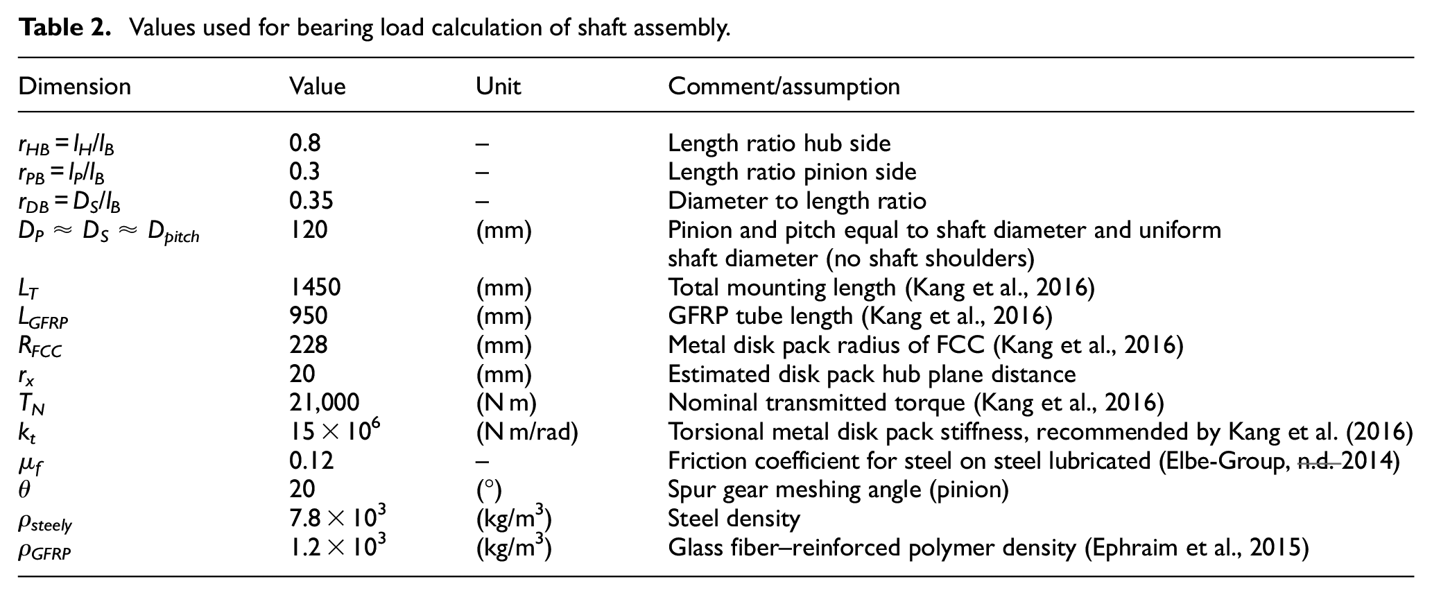
In this section, the previously proposed expressions for the hub and bearing loads as well as estimations of the axial and angular shaft misalignment (displacement) are applied to a specific shaft assembly (Figure 14) using either an FCC or a UJS. Table 2 shows the parameters which are used to compute the hub and bearing loads.

Table 2.

Values used for bearing load calculation of shaft assembly.

Dimension	Value	Unit	Comment/assumption
rHB = lH/lB	0.8	–	Length ratio hub side
rPB = lP/lB	0.3	–	Length ratio pinion side
rDB = DS/lB	0.35	–	Diameter to length ratio
DP ≈ DS ≈ Dpitch	120	(mm)	Pinion and pitch equal to shaft diameter and uniform shaft diameter (no shaft shoulders)
LT	1450	(mm)	Total mounting length (Kang et al., 2016)
LGFRP	950	(mm)	GFRP tube length (Kang et al., 2016)
RFCC	228	(mm)	Metal disk pack radius of FCC (Kang et al., 2016)
rx	20	(mm)	Estimated disk pack hub plane distance
TN	21,000	(N m)	Nominal transmitted torque (Kang et al., 2016)
kt	15 × 106	(N m/rad)	Torsional metal disk pack stiffness, recommended by Kang et al. (2016)
μf	0.12	–	Friction coefficient for steel on steel lubricated (Elbe-Group, 2014)
θ	20	(°)	Spur gear meshing angle (pinion)
ρsteely	7.8 × 103	(kg/m3)	Steel density
ρGFRP	1.2 × 103	(kg/m3)	Glass fiber–reinforced polymer density (Ephraim et al., 2015)

Hub loads calculation

At first, the hub loads are considered, that is, the forces that the joints exert onto the shaft hub(s). This is done for 50% nominal torque, an axial displacement of Δx = 1 mm per FCC joint and an angular displacement angle β = 0. The FCC is aligned at α_FCC = 0° and the UJS at α_UJS = 2.5°. For both FCC and UJS, a dynamic displacement angle of ±0.4° is considered. Furthermore, the hub loads include the effects of joint kinematics (FCC and UJS), metal disk pack deformation (FCC), length compensation (UJS), and weights (FCC and UJS).

Figure 15 shows the hub loads of the FCC and Figure 16 the hub loads of the UJS over the displacement angle α, that is, the gearbox-generator misalignment angle in the horizontal plane. It is visible that the dominant hub load of the FCC is the radial force (F_a/F_r ≈ 0.01–0.02), while the dominant hub load of the UJS is the axial force (F_a/F_r ≈ 20–30). The radial force of the FCC increases significantly with the displacement angle α. This increase is mainly caused by load asymmetry at the connection points (cp. also Figure 13) and thus, by the loads due to disk pack deformation. In contrast, the axial force of the UJS remains almost constant over the displacement angle α. Furthermore, this axial force can be decreased by changing the friction coefficient μ_f in equation (29). Using a UJS with a PTFE (Teflon) coating (cp. also Figure 16) leads to a reduction in the friction coefficient and thus to a decrease in axial and radial hub forces by a factor of 3 (μ_f, _PTFE  = 0.04; Voith (2015)). The friction factor can further be reduced from sliding to rolling friction by installing a tripod UJS (Voith, 2015).

Figure 15.

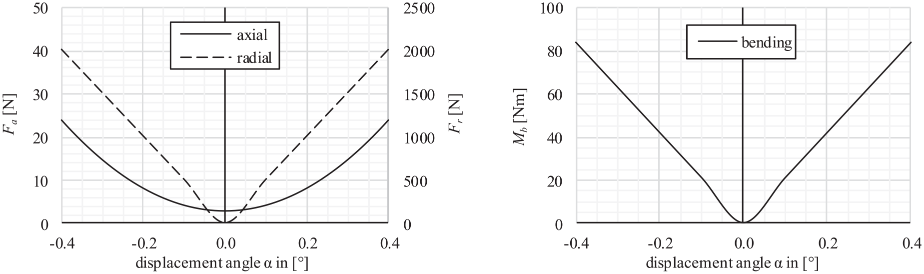
FCC hub forces (left) and bending moment (right) for a range of misalignment angles.

Figure 16.

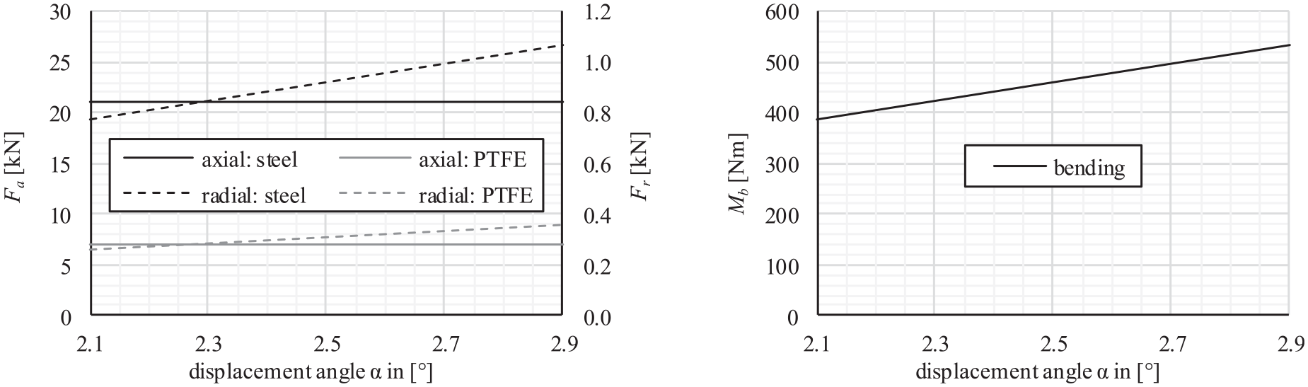
UJS hub forces (left) and bending moment (right) for a range of misalignment angles and an uncoated (steel) versus a PTFE-coated UJS.

Bearing life-time calculation

The bearing loads are calculated for the shaft assembly in Figure 14 using either an FCC or a UJS. Due to the high pinion loads, the radial force on the bearing is much larger than the axial force. Hence, equation (56) should be used, even for the UJS. To compare the bearing loads, that is, the performance of the shaft assembly with an FCC and a UJS, a relative life-time factor is applied in this article. As the (roller) bearing life-time L₁₀ is proportional to the power 10/3 of the inverse value of the equivalent bearing load P (ISO 281), the relative life-time factor f_rel is defined as follows

$$L_{10}~{\left(\frac{1}{P}\right)}^{10/3}$$

(59)

$$L_{10,\mathrm{FCC}}=f_{\mathrm{rel},\mathrm{FCC}}{L}_{10,\mathrm{ref}}$$

(60a)

$$L_{10,\mathrm{UJS}}=f_{\mathrm{rel},\mathrm{UJS}}{L}_{10,\mathrm{ref}}$$

(60b)

$$f_{\mathrm{rel},\mathrm{FCC}}={\left(\frac{P_{\mathrm{ref}}}{P_{\mathrm{FCC}}}\right)}^{10/3}$$

(61a)

$$f_{\mathrm{rel},\mathrm{UJS}}={\left(\frac{P_{\mathrm{ref}}}{P_{\mathrm{UJS}}}\right)}^{10/3}$$

(61b)

The relative life-time factors compare the equivalent bearing loads P_FCC and P_UJS with a reference load P_ref. The reference load P_ref is equal to the ideal FCC case where no misalignment occurs, that is

$$P_{\mathrm{ref}}=P_{\mathrm{FCC}}(\alpha =0,\beta =0,\mathrm{\Delta }x=0)$$

(62)

This means that the reference load P_ref only considers pinion loads and the weights of shaft and FCC (cp. also section “Bearing load calculation”). Note also that a relative life-time factor greater than 1 (f_rel > 1) means that a bearing life-time for the FCC case (L_10,FCC) and UJS case (L_10,UJS), respectively, exceeds the life-time of the reference case (L_10,ref), and vice versa. Next, the relative life-time factor f_rel,FCC will be presented for four different scenarios. Thereafter, the relative life-time factor f_rel,UJS is discussed.

First, the effect of angular displacement is studied by evaluating the relative life-time factor at 50% nominal torque for an axial displacement of Δx = 1 mm per FCC joint (cp. Figure 1). It can be seen in Figure 17 that an increase in the displacement angles α and β of the flexible coupling increases and then decreases the relative life-time factor depending on the sign of the displacement angle α and β. Note that Figure 17 shows this only for the more critical bearing B2 and that the relative life-time factor of bearing B1 behaves opposed to the one of bearing B2 (cp. also Figures 19 and 20). This, however, means that angular displacements cause a variation of the bearing life-time (B1 and B2). Depending on the magnitude and sign of the displacement angles α and β, the life-time can vary several percent.

Figure 17.

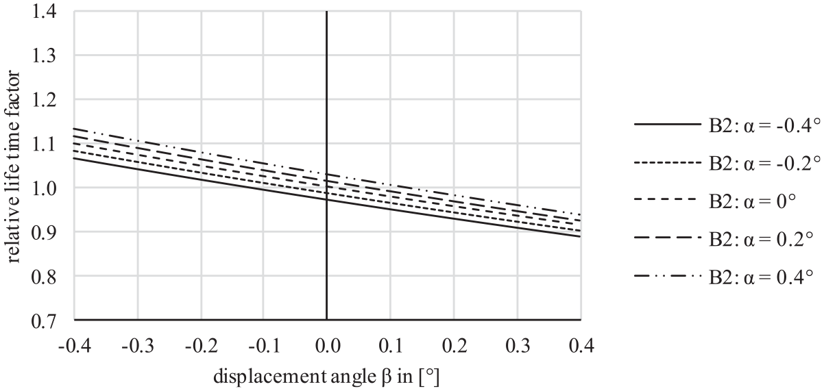
Bearing relative life-time factor as a function of displacement angles α and β at Δx = 1 mm for an FCC.

Second, the influence of an axial displacement is checked by calculating the relative life-time factor at 50% nominal torque for an angular displacement α = 0° (cp. Figure 18). It is shown (for the bearing B2) that depending on the axial displacement Δx (per joint) of the FCC, the relative life-time factor increases and then decreases several tens of percent. This means that the life-time of one bearing increases significantly with an increasing axial displacement Δx, while the life-time of the other bearing decreases. This is because the relative life-time factor of bearing B1 and B2 behave opposed to each other (see Figures 19 and 20). Furthermore, the combination of axial and angular displacement causes significant reaction loads at the shaft end (hub loads) and bearing loads. This can be seen from Figure 18 by comparing line B2: Δx = 0 and B2: Δx = 3 plotted over the displacement angle β.

Figure 18.

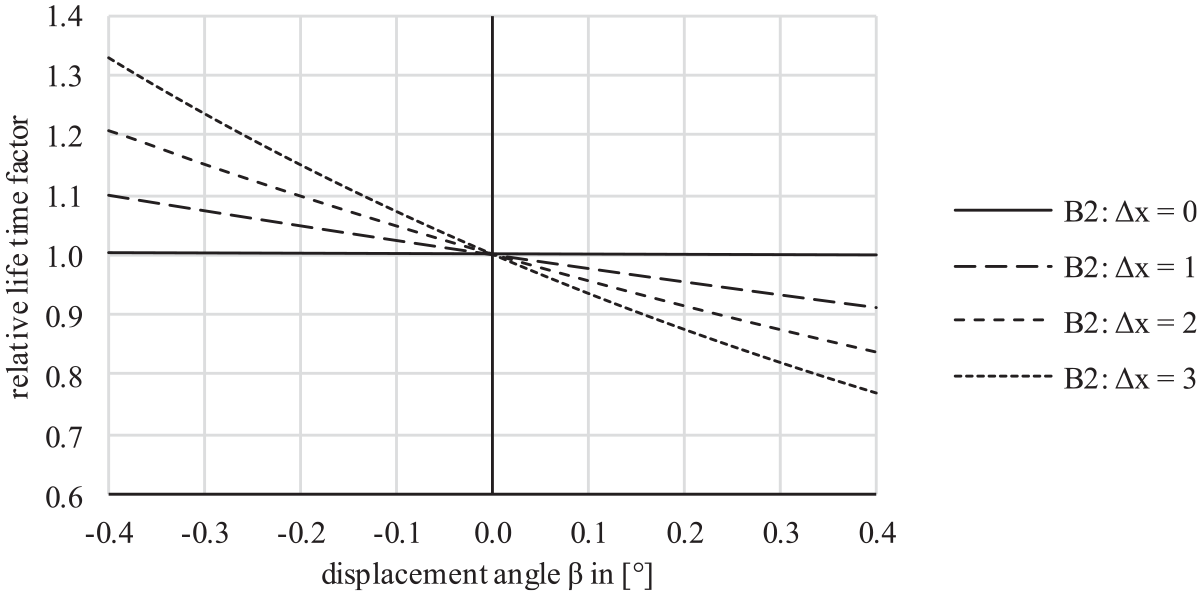
Bearing relative life-time factor depending on axial displacement Δx (mm) and displacement angle β for displacement angle α = 0 for an FCC.

Figure 19.

Bearing relative life-time factor depending on torsional stiffness k_t of the metal disk pack for an FCC.

Figure 20.

Bearing relative life-time factor depending on nominal transmitted torque T_n for an FCC.

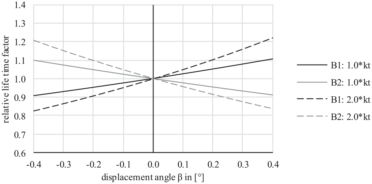
Third, the relative life-time factor is evaluated at 50% nominal torque for an angular displacement α = 0° and an axial displacement Δx = 1 mm. The effect of the disk pack stiffness is investigated for different displacement angles β (cp. Figure 19). By changing the torsional stiffness k_t of the metal disk pack with a factor 2, it can be seen that the relative life-time factor increases and decreases several percent. This means that a high torsional stiffness of the metal disk pack, which is required to transmit high torques and to avoid torsional vibration, has drawbacks for the bearing loads and their life-time.

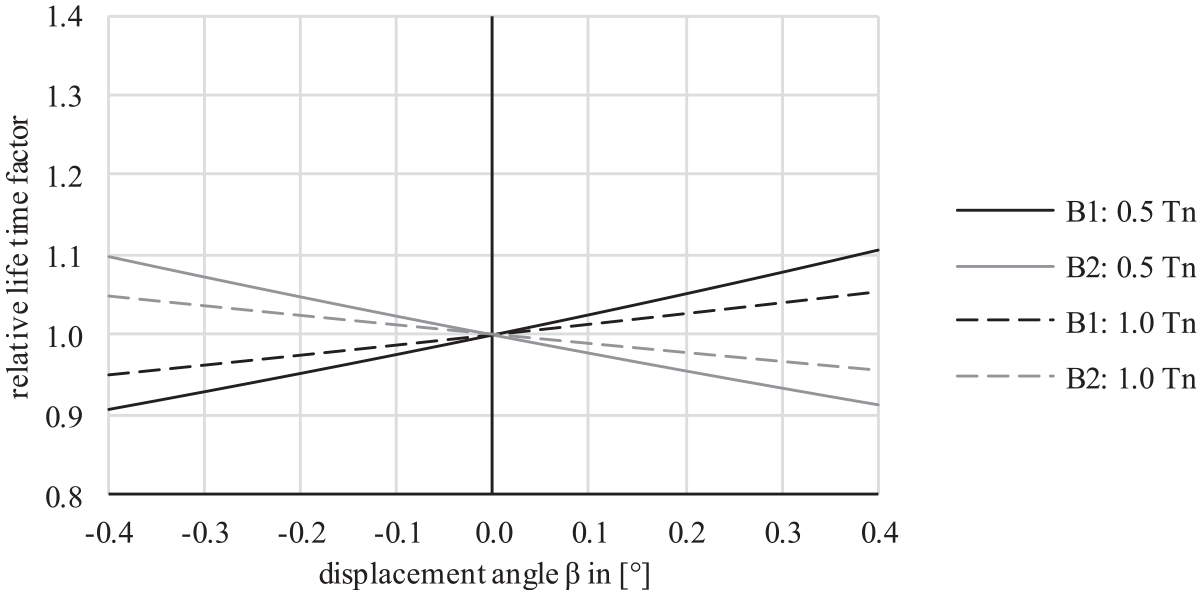
Fourth, the relative life-time factor is calculated at 50% and 100% nominal torque for an angular displacement α = 0° and an axial displacement Δx = 1 mm (cp. Figure 20). Increasing the nominal torque means that the reference load increases, too. Consequently, the relative life-time factor decreases because the hub loads due to disk pack deformation (cp. section “Loads due to disc pack deformations”) are torque independent. Nevertheless, it can be seen from Figure 20 that the hub loads due to disk pack deformation are still notable at nominal torque.

Now, the relative life-time factor for a UJS (f_rel,UJS) is considered. It is evaluated for the displacement angle range α_UJS = 2.5° ± 0.4°. By executing the hub and bearing load calculation (cp. section “Load calculations”) with 50% nominal torque, it can be seen that bearing loads vary less than ±1% within this displacement angle range. This is because of the almost constant hub loads of the UJS (cp. Figure 16). It also means that the bearing loads of the gearbox shaft with a UJS are independent from small dynamic angular displacements during operation and depend only on the transmitted torque (cp. section “Loads due to joint kinematics”). Then, the relative life-time factor is calculated at a displacement angle α_UJS = 2.5° and at 50% nominal torque. It is

$$f_{\mathrm{rel},\mathrm{UJS}}\approx 0.99$$

(63)

It can be seen that the UJS provides an almost constant relative life-time factor f_rel,UJS whose value is close to 1. This means that the UJS performs similar to an FCC at ideal operation conditions, where neither axial (Δx = 0) nor angular (α = 0, β = 0) misalignments occur.

Discussion

By considering the relative life-time factor, it can be seen that using an FCC causes a large variation of HSS bearing loads, while using a UJS provides almost constant bearing loads. The reaction loads of the FCC are dominated by the metal disk pack deformation, that is, they are mainly influenced by the axial and angular displacement between gearbox and generator HSS. The reaction loads of the UJS, however, depend mainly on the transmitted torque, that is, the influence of small displacements during operation can be neglected. Due to the high variation of the HSS bearing loads, the bearing life-time varies, too. This means that bearing life-time predictions are difficult and that the bearings fail rather randomly which leads to unplanned downtimes. In contrary, constant and torque-dependent bearing loads allow a more accurate bearing life-time prediction which may result in planned instead of unplanned downtimes.

Furthermore, for typical combinations of axial and angular displacements during operation, that is, 1–2 mm axial displacement per FCC joint and approx. 0.3°–0.4° angular displacement (cp. also section “Displacement Estimation”), the FCC causes relative life-time factors of approx. 0.75. It can be expected that even lower relative life-time factors occur because FCC suppliers allow higher displacements than considered in this article. In the case of the FCC shown in Figure 2, the maximal permissible displacements, given by the supplier, are 5 mm axial (per joint) and 1.0° angular (Kang et al., 2016). Suppliers also state that the flexible connecting coupling should not operate simultaneously at the maximal permissible axial and angular displacement. So assuming that the flexible connecting coupling operates around the half of the permissible displacements, that is, 2–3 mm axial (per joint) and approx. 0.5° angular, which is likely after section “Displacement estimation,” relative life-time factors of approx. 0.6–0.7 can still occur. In other words, the usage of the FCC can reduce the gearbox bearing life-time to approx. 60%–70% of the designed life-time.

Moreover, it can be seen from Figure 17 that the displacement angle β has a larger effect on the relative life-time factor than the displacement angle α. The reason for this effect is the direction of the reaction force due to metal disk pack deformations. The reaction force due to the displacement angle β is parallel to the main reaction force of the pinion, while the reaction force due to the displacement angle α is perpendicular (cp. sections “Loads due to disc pack deformations” and “Bearing load calculation”). Consequently, the reaction force due to the displacement angle β has a larger influence on the bearing loads than the reaction force due to the displacement angle α. In a wind turbine, the displacement angles α and β are caused by main shaft or base frame bending. However, as the wind turbine gearbox is fixed in rubber bushes, the displacement angle β is also generated by the deformation of the rubber bushes due to the gearbox counter torque. The counter torque is equal to the ring gear torque of the planetary gears used in wind turbine gearboxes at the first (and second) gear step. This means that the magnitude of the counter torque is similar to the magnitude of the wind turbine rotor torque depending on the stationary gear ratio of the planetary gear(s). Consequently, significant (static and dynamic) displacement angles β can occur during operation depending on the rubber bushes stiffness, that is, operation at a displacement angle β around ±0.4° seems likely.

In addition to improving wind turbine designs, the calculation method for hub (coupling joint) and bearing loads proposed in this article can also be used to predict the remaining useful life-time of gearbox (and generator) bearings. The transmitted torque can be derived from SCADA data, that is, from the speed of the gearbox HSS and transmitted power. The axial and angular misalignment is estimated (a) with the alignment protocol filled in by technician during installation and (b) with the dimensions of the FCC, the speed of the main shaft (from SCADA) and gearbox vibration data measured by the condition monitoring (CM) system (cp. also section “Displacement estimation”). Then, the hub and bearing loads are determined with the torsional disk pack stiffness (available in data sheets) and the HSS dimensions (cp. sections “Loads due to joint kinematics,”“Loads due to disc pack deformations,” and “Bearing load calculation”). Based on these loads and the bearing type (load capacity), the bearing life-time can be calculated using ISO 281 and therefore also the remaining useful life-time. This process is shown schematically in Figure 21.

Figure 21.

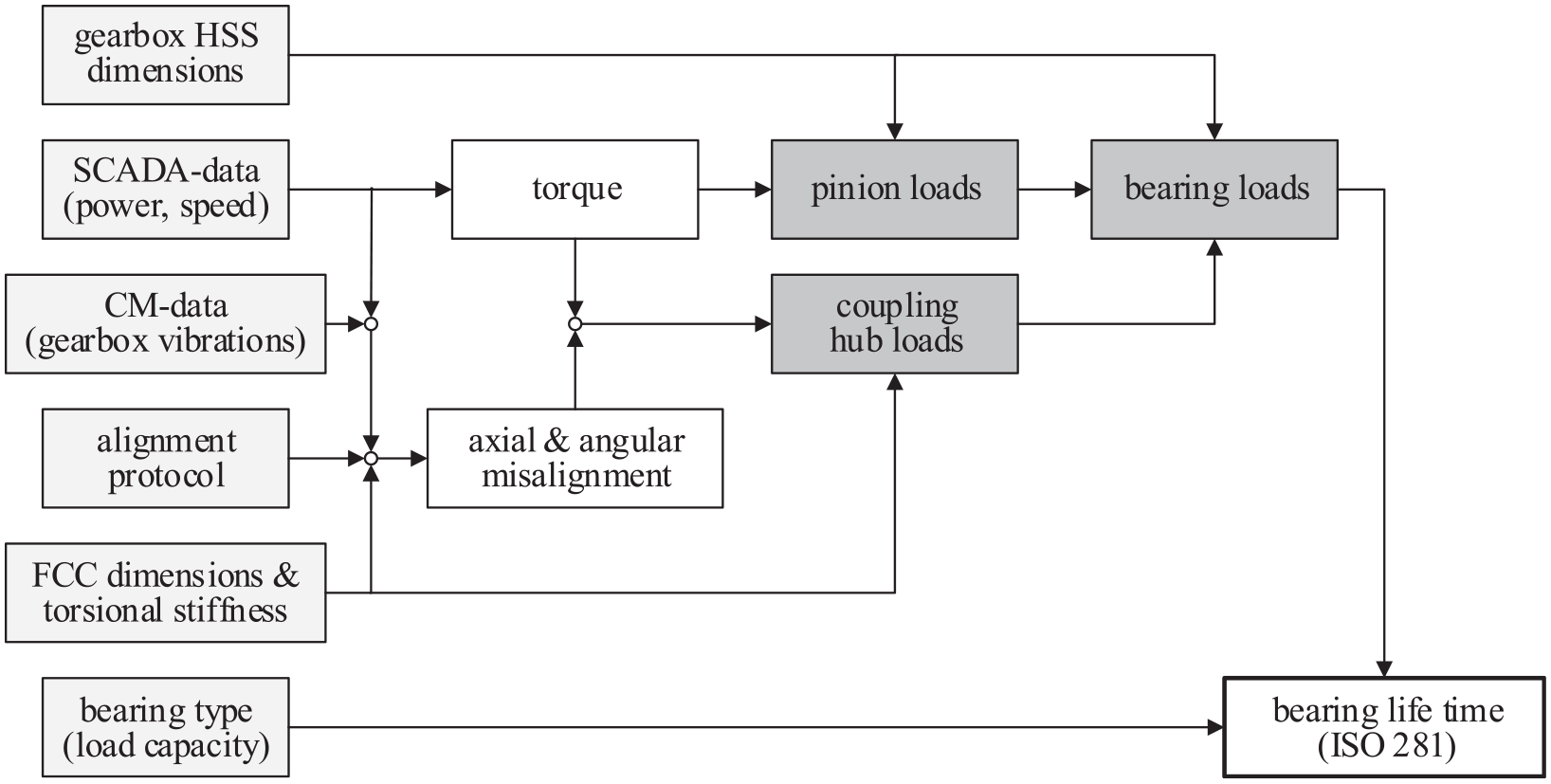
Prediction of remaining useful bearing life-time based on SCADA, CM-data, and component dimensions.

Finally, as at present no explicit equations to calculate the coupling hub loads were available, the bearing loads could not be calculated accurately. This has led to big deviations between predicted/expected (during design) wind turbine gearbox life-times and the actual (much shorter) life-times observed in the field. The method proposed in this work enables a quick and accurate calculation of these hub loads, leading to much more accurate gearbox bearing life-times.

Conclusion

This article provides a calculation method to evaluate the bearing load increase (life-time reduction) caused by shaft connecting couplings and the axial and angular misalignment of gearbox and generator HSS. The method takes into account the reaction loads of the coupling joints due to both kinematics (UJS and FCC) and metal disk pack deformations (FCC). The metal disk packs are modeled as 1D tension/compression springs whose stiffness is obtained from the torsional stiffness of the metal disk pack (given in data sheets). The shaft misalignment is estimated based on HSS alignment during installation and on vibration data during operation. The load calculations are shown to be part of the remaining useful life prediction of gearbox (and generator) HSS bearings considering SCADA, CM data, as well as HSS component dimensions.

To demonstrate the proposed approach, the load calculations are applied to a specific FCC and UJS. By comparing their performance it is shown that the usage of FCCs can significantly increase the bearing loads of gearbox and generator HSS in wind turbine drive trains. The bearings can fail at 60%–70% of the design life-time because high bearing load fluctuations occur, caused by the displacement during operation. Furthermore, it is demonstrated that the reaction loads of FCCs are dominated by metal disk pack deformations, that is, they are dependent on small displacements during operation. In contrast, the reaction loads of UJS are governed by the transmitted torque and independent of small displacements during operation. This means that (in the case of the UJS) the gearbox and generator bearing loads are not affected by small shaft displacements during operation. Finally, it is discussed that the usage of a UJS (a) allows a more accurate prediction of bearing life-time because the loads of UJS are torque dependent and displacement independent and therefore (b) avoids costly, unplanned gearbox and generator failures as well as downtimes.