
Abstract
This work demonstrates a technique to identify information about the ice mass accumulation on wind turbine blades using its natural frequencies, and these frequencies reduce differently depending on the spatial distribution of ice mass along the blade length. An explicit relation to the natural frequencies of a 1-kW wind turbine blade is defined in terms of the location and quantity of ice mass using experimental modal analyses. An artificial neural network model is trained with a data set (natural frequencies and ice masses) generated using that explicit relation. After training, this artificial neural network model is given an input of natural frequencies of the iced blade (identified from experimental modal analysis) corresponding to 18 test cases, and it identified ice masses’ location and quantity with a weighted average percentage error value of 17.53%. The proposed technique is also demonstrated on the NREL 5-MW wind turbine blade data.
Keywords
Introduction
Wind turbines are increasingly installed in the northeastern and the mid-Atlantic United States, Canada, and Northern Europe due to good wind resources and land availability. In these regions, humidity along with low temperatures in the winter increases the risk of ice accumulation on wind turbine components. The global wind energy installations in cold climate regions reached a capacity of 127 GW at the end of 2015, and the forecast is that it would reach a capacity of 186 GW by the end of 2020 (Emerging from the Cold, 2016). Icing of the rotor blades results in reduced turbine power output as it reduces the lift force and increases the drag force acting on blade’s airfoil sections (Rindeskär, 2010; Turkia et al., 2013). Additionally, the nacelle vibration amplitudes increase during the icing conditions (Skrimpas et al., 2015), so icing can be more reliably detected using the power curve analysis along with nacelle vibration analysis. Etemaddar et al. (2014) investigated the effects of atmospheric ice accumulation on the aerodynamic performance and structural response of the wind turbines, and they predicted that the relative change in mean value is higher than the change in standard deviation for most of the response quantities (rotor speed, torque, power, thrust, and structural loads) of the iced blade. Gantasala et al. (2016) analyzed the modal behavior of a 2-MW wind turbine blade under icing conditions. Their analysis showed that the aeroelastic damping factors of the vibration modes reduce with ice accumulation on the blade. Rissanen et al. (2016) proposed simulation parameters for predicting the dynamic behavior of iced wind turbines to generate icing design load cases for the new IEC 61400-1 ed4.
Ice accumulation on the wind turbine blades is not uniform and its mass distribution changes under different stages of icing and ice shedding during operation. The natural frequencies of a blade reduce according to the quantity and location of ice mass along its length. Lorenzo et al. (2013) investigated the influence of ice mass on the natural frequencies of the NREL 5-MW turbine by extracting model parameters from the operational modal analysis. Alsabagh et al. (2015) considered different ice mass distributions as defined in the ISO 12494:2001 (2001) standard on a multi-megawatt wind turbine blade. They analyzed the influence of ice mass on natural frequencies and dynamic magnification factors (ratio of the dynamic deflection to static deflection), by considering only the mass changes in the blade. Wind turbines are usually exposed to turbulent wind conditions which will excite natural frequencies of the blade, and these frequencies can be extracted from the blade’s vibration measurements. The ice detection systems like BLADEcontrol (Brenner, 2016), fos4blade IceDetection (Cattin and Heikkilä, 2016; fos4X data sheet, n.d.), and Wolfel IDD.Blade (Wölfel, 2016) detect ice based on the deviations in blade’s natural frequencies. These systems can detect icing while the turbine is in operation or at a standstill condition, which enables automatic restart of the turbine once the blades are ice-free after de-icing. These systems indicate the state of icing on the blades such as ice-free, non-critical ice, and critical ice, but cannot identify the location and quantity of ice mass. The most widely used anti-icing and de-icing systems work on the basis of heating resistance or hot air blowing techniques (Ilinca, 2011). Both these systems require an external power source (with a capacity of 150–225 kW for a typical 3-MW range wind turbine (Nielsen, 2017; Roloff, 2017)) and consume 1%–4% of annual energy production, depending on the icing severity (Peltola et al., 2003). The required power to remove ice can be minimized if the location and quantity of ice mass are determined approximately so that the relevant energy needed at the appropriate locations of the blade can be supplied to remove ice. In addition to that, the de-icing process can be initiated and monitored remotely without the need of turbine maintenance personnel’s physical presence at the site. This has motivated the authors to pursue an idea to determine the location and quantity of ice mass accumulated on wind turbine blades.
Fan and Qiao (2011) summarized various damage identification methods for beam- or plate-type structures that use different vibration features (natural frequency–based methods, mode shape–based methods, curvature mode shape–based methods, and methods using both mode shapes and frequencies). These methods rely on the effect of damage induced changes in the physical properties of the structure (mass, damping, and stiffness) on its modal properties. If the changes in physical properties are known, their effect on modal properties can be estimated using either mathematical models of the structural behavior (like finite element method (FEM) models) or experiments (like modal analysis), which is depicted as a forward problem in Figure 1(a). Damage identification methods rely on the inverse problems (as shown in Figure 1(b)) where the location and severity of a damage in the structure are determined based on its modal properties. The authors of this article used an artificial neural network (ANN) model in Gantasala et al. (2017) to solve such inverse problem for identifying added masses on a cantilever beam for any given set of natural frequencies of the corresponding beam. Initially, a data set of natural frequencies of the beam is created using its FEM model where different quantities of added masses are considered at different locations on the beam. A neural network model is trained with this data set considering natural frequencies of the beam as an input and corresponding added masses used in the calculations as an output. It approximates a nonlinear relationship between these inputs and outputs which can be used to identify added masses for any given set of natural frequencies of the beam consisting added masses. This method has a limitation that it requires an updated FEM model (eigenvalues of the FEM model closely match with those estimated from experimental modal analysis of the structure) to create the data set required for training the neural network. The requirement of an FEM model of the structure makes it practically difficult to use such technique for ice detection on wind turbine blades as its FEM model is a proprietary information of the manufacturer. In this work, the authors propose a new method to create the data set required for training the neural network. Experimental modal analyses (output only) are conducted on a small-scale wind turbine blade considering two different quantities of ice mass at three different locations along the blade (ice mass is considered in one location at a time). Later, the relations between natural frequencies of the wind turbine blade and the quantity of ice mass used in each location are obtained using polynomial fitting (natural frequencies are considered as dependent variables and ice masses are considered as independent variables). These relations are used to create a data set of blade’s natural frequencies considering different quantities of ice masses at three different locations along the blade. A neural network model is trained with that data set and used to identify ice masses for a given set of natural frequencies of the blade estimated from experiments (different ice masses are considered randomly along the three different locations defined on the blade). Those ice masses are compared with the actual ice masses considered in the experiments.
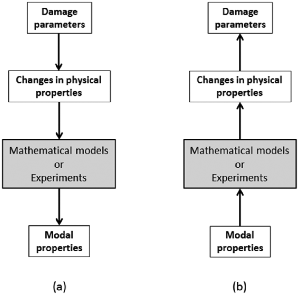
(a) Forward problem and (b) inverse problem.
Experimental setup and modal analysis
A 1-kW wind turbine blade as shown in Figure 2 is considered in this study and its root is rigidly fixed to a stationary support. Geometric details of the blade are given in Table 1. Four uni-axial accelerometers (Bruel & Kjær Type 4507) are placed on the blade to measure vibration accelerations in the flapwise direction using a National Instruments NI-9234 data acquisition card along with the DEWESoft7 data acquisition software.
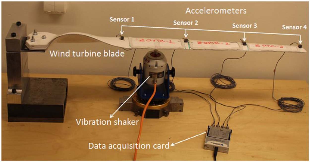
Experimental modal analysis setup.
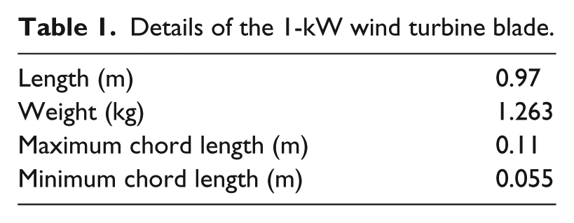
Details of the 1-kW wind turbine blade.
Two different output only modal identification techniques are used in this section to extract modal parameters of the blade from experimentally measured vibration accelerations (excitation forces are not measured). In the first method, the blade is excited with a low-pass filtered (up to 200 Hz, as first three flapwise modes of the blade are within this frequency range) Gaussian white noise force using a vibration shaker (TIRAvib S-50018) as shown in Figure 2, and its vibration accelerations are measured using four accelerometers with a sampling frequency of 2048 Hz for 200 s. The measured signals for a short duration of 4 s are shown in Figure 3. Modal parameters of the blade (natural frequencies and mode shapes) are extracted using a frequency-domain decomposition (FDD) technique on the measured vibration accelerations. It identifies modal parameters in the frequency domain using a non-parametric model. The measured vibration signals are divided into segments to calculate power spectral density (PSD) estimates using Welch’s overlapped segment averaging estimator. The PSD matrix calculated at discrete frequencies within the sampling frequency is decomposed by means of a singular value decomposition (SVD). These singular values are the estimates of the auto spectral densities of the single-degree-of-freedom (SDOF) systems, whereas singular vectors are estimates of the structural mode shapes. The PSD matrix at any frequency is mainly dominated by the vibration modes around that frequency. Near the resonance frequencies of the structure, the SVD of the PSD matrix will return a predominant singular value signifying a single vibration mode contributes to the PSD matrix at that frequency and the corresponding mode shape is characterized by its singular vector. The authors used an open-source MATLAB code written by Cheynet (2016) for modal parameter identification using the FDD, and further theoretical details on the FDD technique can be found in Brincker et al. (2001). The singular values calculated in the current case for the PSD matrix at various frequencies are shown in Figure 4, where first three flapwise natural frequencies of the blade can be identified at the peaks in the first singular value.
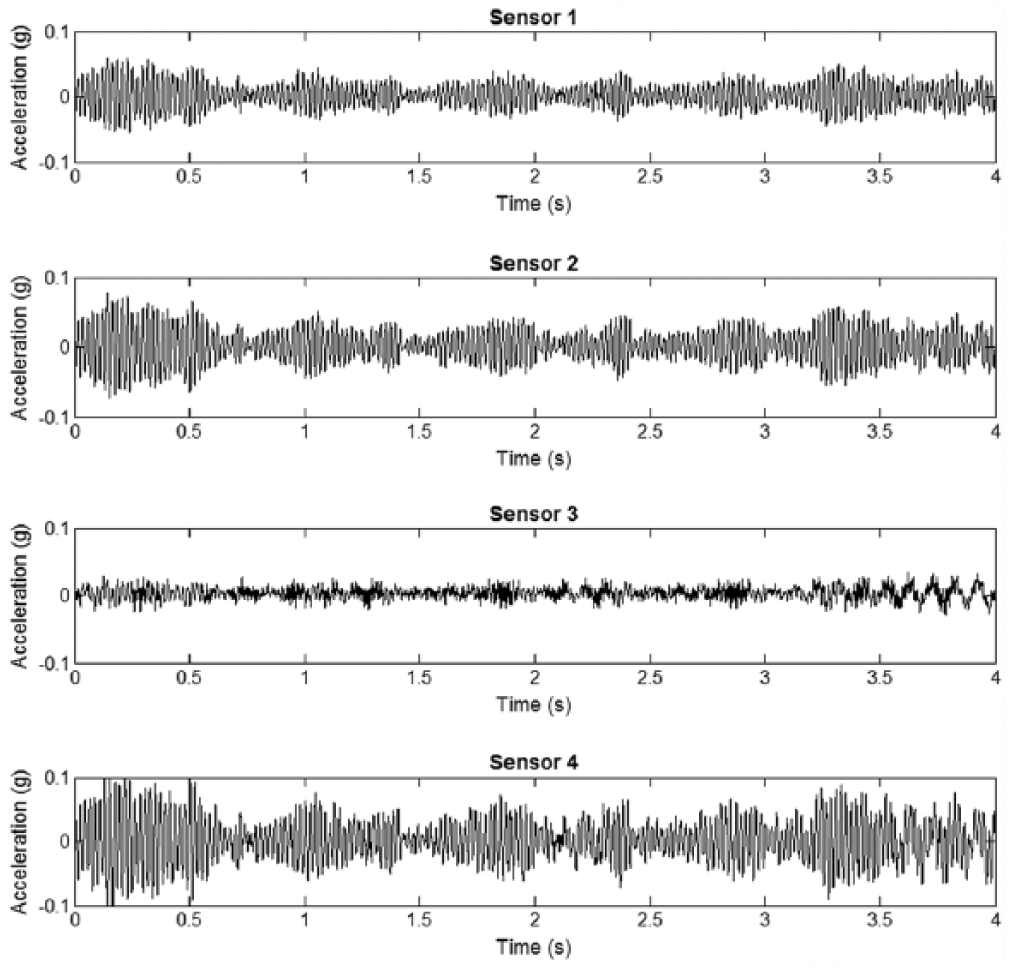
Vibration accelerations of the blade for a low-pass filtered Gaussian white noise excitation.
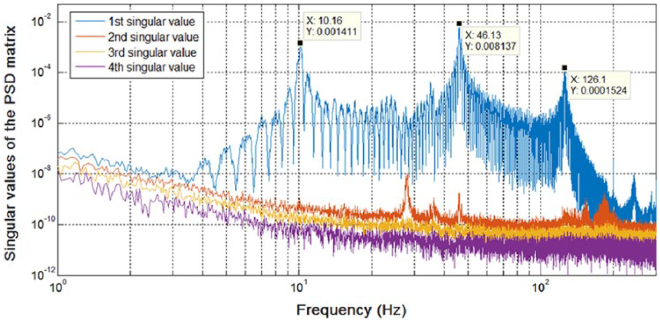
Singular values of the PSD matrix.
In the second modal identification method, the blade is excited with an impact hammer and its free vibration responses are measured. Impact hammer is only used to excite free vibrations of the blade, and its forces are not measured. After an impact hit on the blade, data acquisition system is triggered to acquire free vibration responses with a sampling frequency of 2048 Hz for 6 s (free vibration responses are decaying within this duration). The measured vibration accelerations for a short duration are shown in Figure 5. These measured vibration accelerations are used in an open-source Structural Modal Identification Toolsuite (SMIT) written by Chang et al. (2012). That toolsuite consists of five different time-domain-based output only system identification algorithms (their theoretical background is presented in Chang and Pakzad (2014)). In this study, subspace state space system identification (N4SID-OO) algorithm available in that toolsuite is chosen for extracting modal parameters of the blade. A state space model of certain order is assumed to model the vibration behavior of the test structure in the subspace method where it identifies the state space matrices corresponding to the test structure based on its discrete time-sampled vibration signals. The measured vibration signals are arranged in the form of a Hankel matrix with an even number of rows, and it is further divided into two sub-matrices (consisting equal number of rows), where the upper sub-matrix is called as past output and the lower sub-matrix is called as future output. Using an SVD on the projection of row space of future outputs onto the row space of the past outputs, state space matrices corresponding to the test structure are obtained, from which modal parameters are extracted. This algorithm is not described here in detail as it is out of the scope of this article, more details on this algorithm can be found in Van Overschee and De Moor (1994).
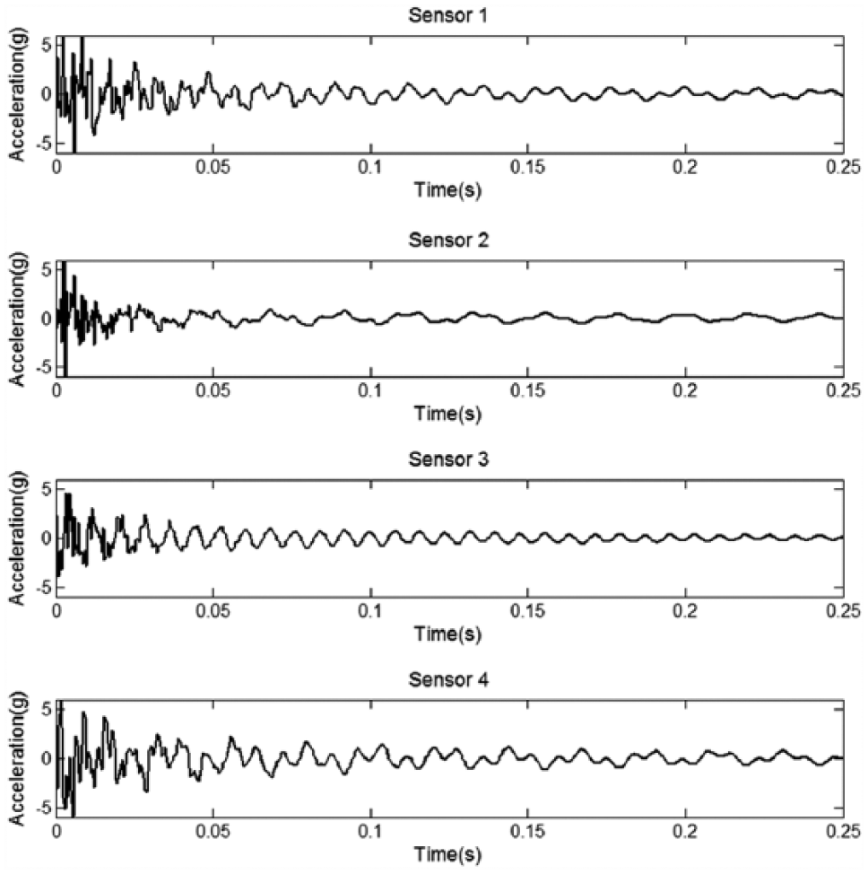
Free vibration accelerations of the blade measured using four sensors.
A stability diagram is plotted in Figure 6 to identify true poles of the system for different model orders. Three dominant peaks can be identified at 10.1698, 46.1688, and 125.96 Hz in the PSD plot which matches with the stable poles (for all model orders above 10) identified in the subspace identification algorithm, and they correspond to the first three flapwise modes of the blade.
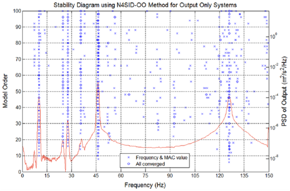
Stability diagram for the modes of the system.
The natural frequencies identified using both modal identification methods are compared in Table 2, and their mode shapes are plotted in Figure 7. The modal parameters identified using two modal identification methods match very well with each other. The difference between these identified frequencies is marginal, and the mode shapes are only deviating at the location of sensor 2 in second and third modes. The authors are only interested in the natural frequencies of the blade, and mode shapes are extracted for confirming those frequencies correspond to first three vibration modes of the blade. One of these two identification methods can be used for further experiments with ice on the blade, the authors chose time-domain-based modal identification technique compared to the other method as it is more convenient and quicker to measure free vibration responses (for a duration of 6 s only) of the blade.
Comparison of natural frequencies of the 1-kW wind turbine blade identified using FDD and N4SID-OO modal identification methods.
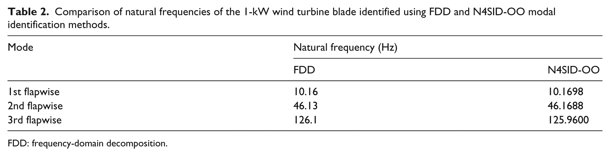
FDD: frequency-domain decomposition.
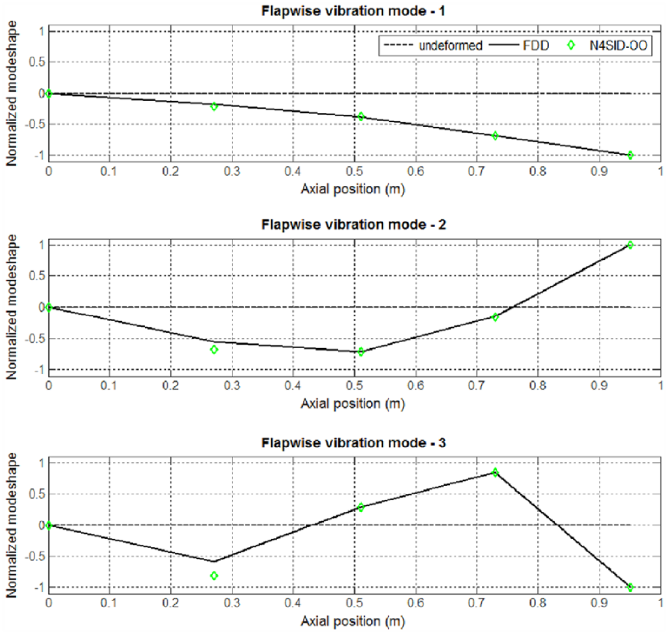
Comparison of mode shapes identified using FDD and N4SID-OO modal identification methods.
Experimental modal analysis of the blade with ice mass
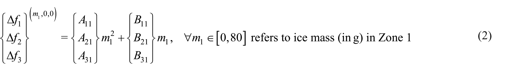
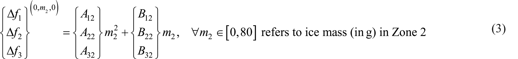
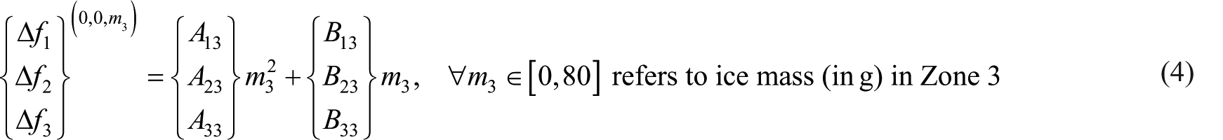
Three different zones of length 0.2 m are defined along the blade as shown in Figure 8, where two quantities of ice masses 40 and 80 g are placed (randomly distributed) in each of these three zones separately (refer to Figure 9(a) to (c)). These ice masses are not naturally formed on the blade, instead ice formed during the winter season is collected and placed on the upper side of the blade’s flapwise surface. Experimental modal analysis is carried out in the six cases described before (two quantities of ice masses are considered in three zones), and the measured free vibration responses are used in the Subspace State Space System Identification (N4SID-OO) algorithm (Chang et al., 2012) to extract corresponding modal parameters of the blade. First three flapwise natural frequencies of the blade identified in these six cases are given in Table 3. These natural frequencies are reduced differently depending on the location and the quantity of ice mass. A quadratic polynomial as shown in Figure 10 is fitted separately between each one of the three natural frequencies of the iced blade corresponding to the cases of ice mass considered in a specific zone and respective ice masses (0, 40, and 80 g) used in that zone. In total, nine polynomials are fitted between three natural frequencies of the iced blade and respective ice masses used in the three zones. These polynomials can be expressed in the form of equation (1), and they can be used to interpolate natural frequencies of the iced blade corresponding to any intermediate ice mass value between 0 and 80 g. The reduction in natural frequencies of the blade for any ice mass value between 0 and 80 g in any one of the three zones exclusively can be calculated using the polynomial coefficients (their values in the current case are given in Appendix 1) given in equations (2) to (4)

where
where
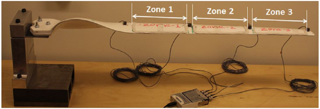
Definition of three zones along the blade length.
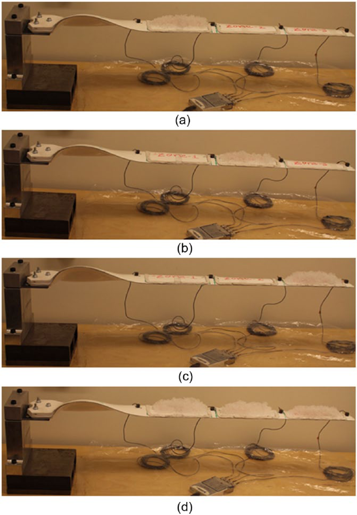
Ice masses considered along the blade in (a) Zone 1, (b) Zone 2, (c) Zone 3, and (d) Zones 1, 2, and 3.
Influence of ice mass on first three flapwise natural frequencies of the 1-kW wind turbine blade.
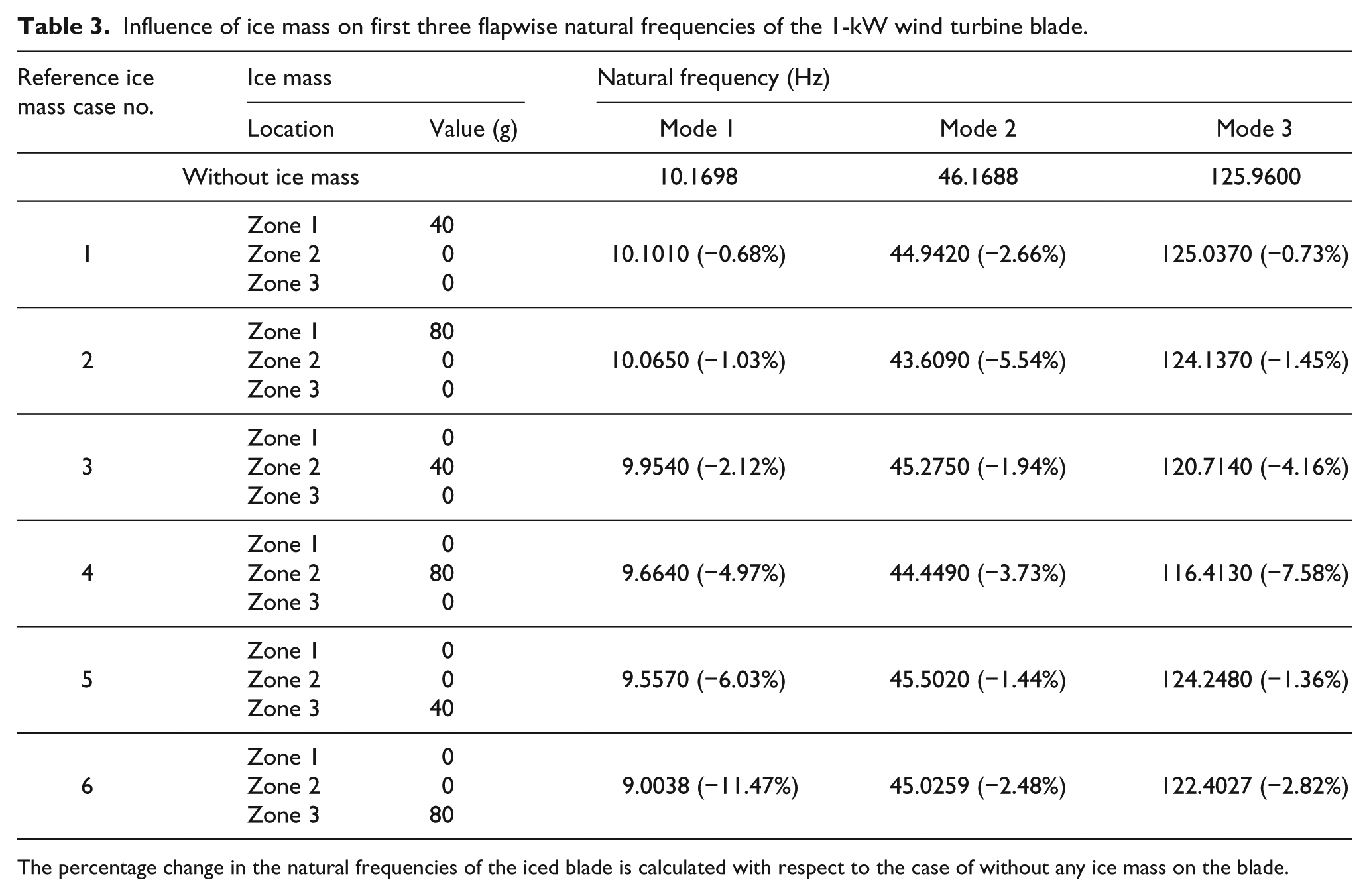
The percentage change in the natural frequencies of the iced blade is calculated with respect to the case of without any ice mass on the blade.
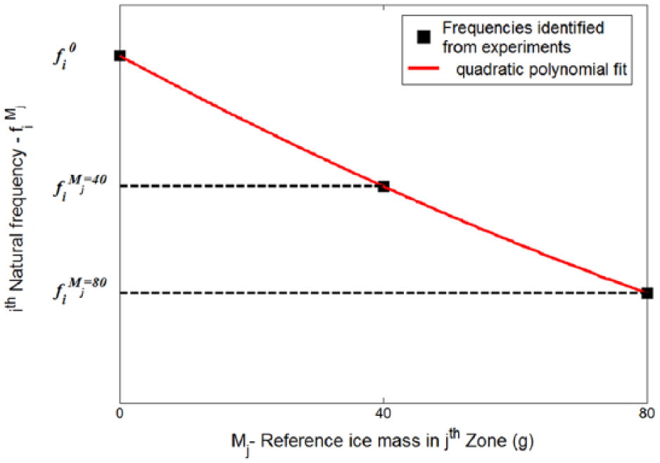
Quadratic polynomial curve fit for the
Using equations (2) to (4), the natural frequencies of blade with ice masses
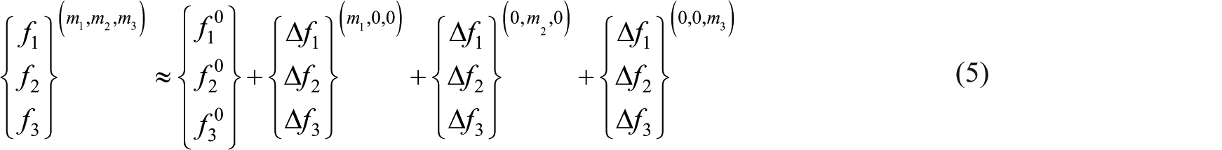
where
Comparison of natural frequencies of the blade with 40-g ice mass in all three zones calculated using equation (5) and identified from the experimental modal analysis.
A valid forward relation between ice masses (as independent variables) and natural frequencies (as dependent variables) of the 1-kW wind turbine blade is defined in this section using experimental modal analyses with ice masses. So, first three natural frequencies of the iced blade can be determined using such relation without in need of a structural model like FEM when the quantities of ice masses are known. Similarly, an inverse relation with ice masses as the dependent variables and natural frequencies as the independent variables is required to find the quantities of ice masses whenever natural frequencies of the iced blade are known. It is difficult to express these inverse relations explicitly. However, optimization techniques can be used to serve the purpose of finding the quantities of ice masses which will reduce the natural frequencies in the similar way as that of measured frequencies of an iced blade. A cost function can be defined using the forward relation and target natural frequencies where ice masses are chosen as variables in the optimization techniques and tuned to match the frequencies calculated using the forward relation with target frequencies. This process needs to be repeated for every new set of target frequencies to find corresponding ice masses which makes it cumbersome to use for ice mass detection. Another viable option is to define the inverse relation between ice masses and natural frequencies using an artificial neural network (ANN) model which expresses that relation explicitly, so it is straightforward to use that relation later for detecting ice masses for any new input of natural frequencies of the iced blade.
ANN model
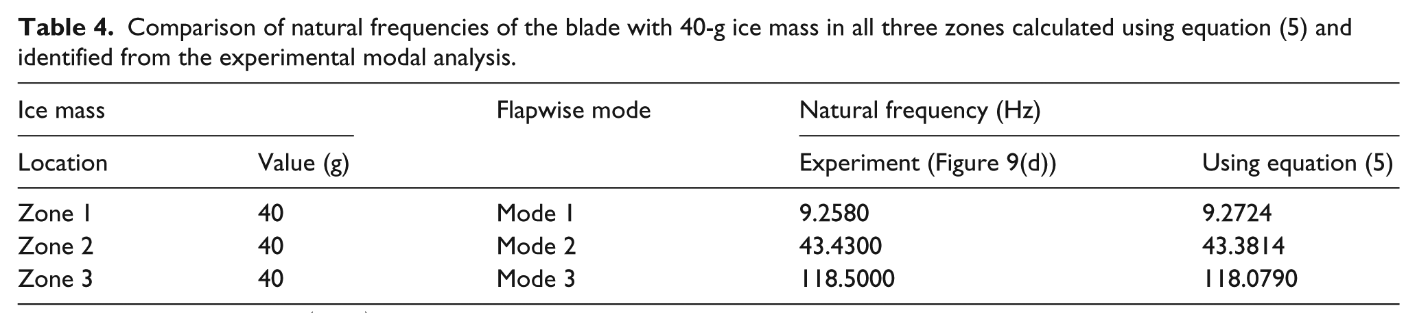
ANNs are inspired from the biological neural networks, where artificial nodes known as neurons are used as computational elements and connected together to form a network. The ANN can be used to estimate or approximate functions that depend on multiple variables. These networks receive input from the neurons in the input layer, and their output are given by the neurons in the output layer. There may be one or more intermediate hidden layers. The neuron behaves as an activation or mapping function (typically a nonlinear function) producing an output corresponding to the input to the neuron. The neurons in the network are connected with each other and associated with some weights and bias which either increase or decrease input signals to the neurons. These weights and bias are determined in the training process where the relation between input and output variables is established (Ata, 2015). The backpropagation algorithm is one of the most widely used algorithms to determine the weights and bias of the neurons organized in layers. In this algorithm, the network signal travels in the forward direction and the errors are propagated backward. This algorithm uses supervised learning in which the network is trained using data for which inputs as well as desired outputs are known. The backpropagation algorithm is a generalization of the least mean square algorithm that modifies network weights to minimize the mean square error
A simple network with two neurons in a hidden layer is shown in Figure 11. The input to the network is
A simple artificial neural network model.
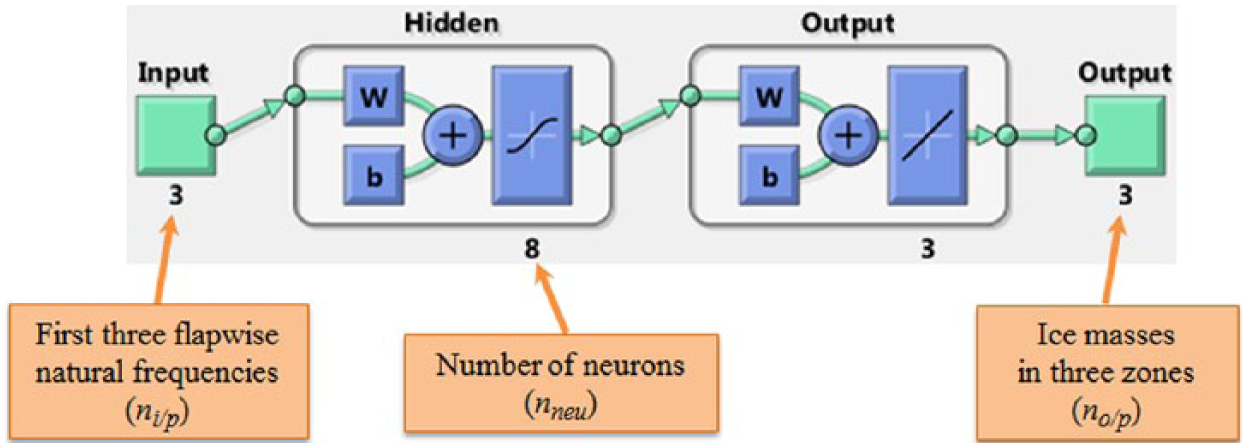
In this study, a nonlinear function that considers natural frequencies of the iced blade as an input and the ice masses accumulated in the three zones defined on the blade in corresponding cases as an output is approximated using ANN. As discussed before, the network parameters need to be found by trial and error method, which makes the process of finding network parameters cumbersome. However, based on the training data and problem under consideration, these parameters can be chosen, which is outlined as follows:
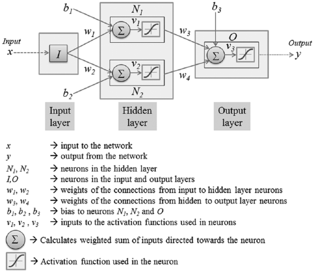
Gantasala et al. (2017) found
Different cases possible when two values are chosen for an ice mass in each one of the three zones.
Neural network designed using the MATLAB toolbox.
Results and discussion
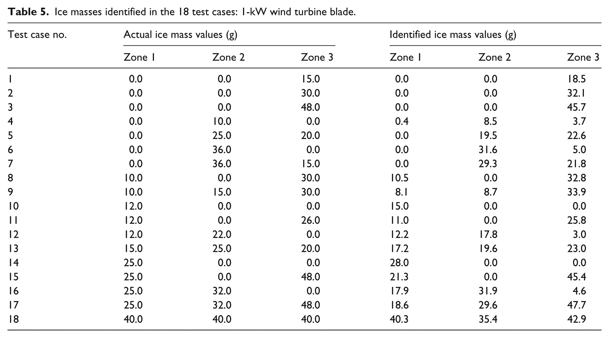
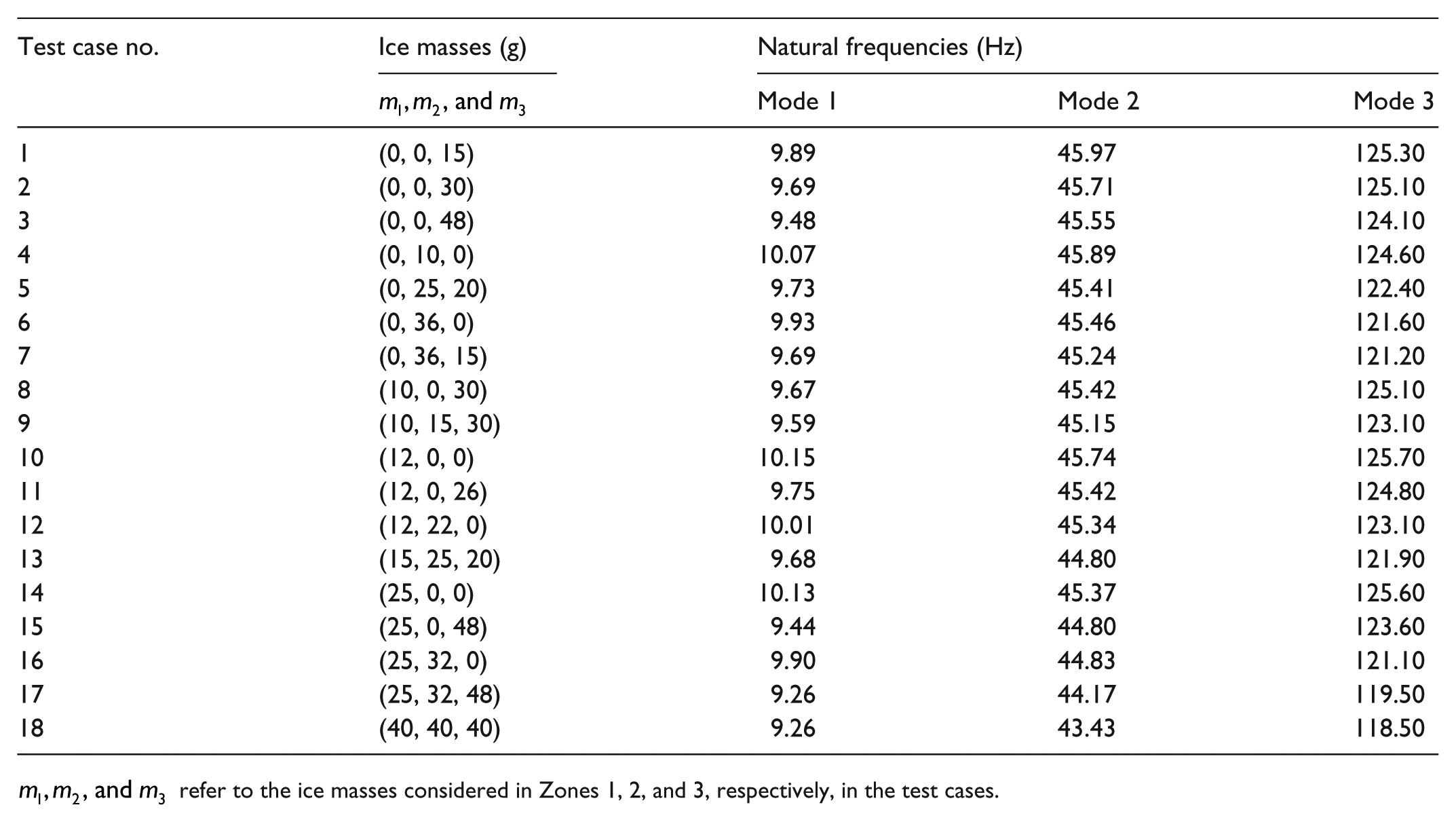
In this section, 18 cases of ice masses (randomly chosen between 0 and 80 g in all three zones) are considered along the length of the three zones defined on the 1-kW wind turbine blade, and its first three flapwise natural frequencies are identified from the experimental modal analysis. These ice masses are distributed randomly (i.e., linear mass density varies randomly) along the length of the zones. The natural frequencies identified in the above cases (given in Appendix 2) are given as an input to the neural network model designed in the last section, and the identified ice masses are compared against the actual ice mass values used in the experiments in Table 5. As the actual ice mass values used in the experiment and the corresponding identified mass values in all 18 test cases are known, an error metric called as weighted absolute percentage error
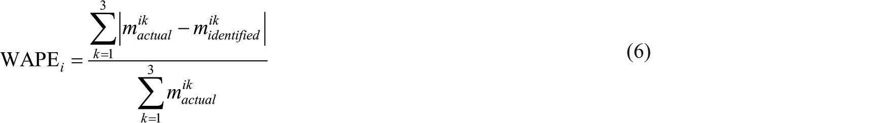
where
Ice masses identified in the 18 test cases: 1-kW wind turbine blade.
The WAPE is calculated for all 18 test cases and shown in Figure 14. This error changes with respect to the location and the quantity of ice mass, and the mean value of WAPE for all 18 cases is found to be 17.53%. Ice masses in the test case 4 are identified with a maximum WAPE value of 55.6%, where only 10 g of ice mass is considered in Zone 2 in the experiment. It can be observed that the WAPE value is higher in test cases where smaller ice masses are considered on the blade and it decreases with increasing ice mass values. The randomness in the way ice masses are distributed in the experiments resulted randomness in the WAPE values of 18 test cases. The proposed ice mass detection algorithm is able to approximately identify ice masses in the three zones defined on the blade based on its first three flapwise natural frequencies. Its application to a large wind turbine blade is demonstrated in the next section.
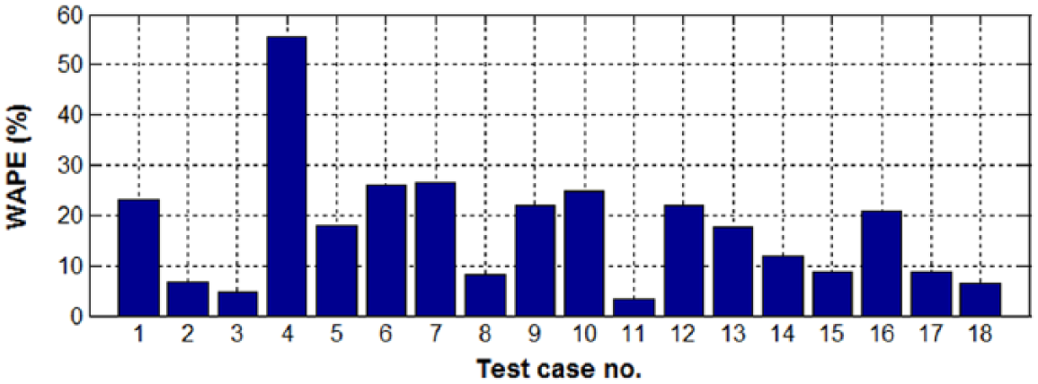
Weighted absolute percentage error
Application of the proposed technique to detect ice masses on a multi-megawatt wind turbine blade
The detection technique proposed in the earlier sections is approximately able to identify ice masses on a 1-kW wind turbine blade, the same technique is used in this section for detecting ice masses on the NREL 5-MW wind turbine blade. In the case of 1-kW wind turbine blade, an explicit relation between natural frequencies and ice masses is defined using experimental modal analyses of the iced blade; here, in this section, such relation for the NREL 5-MW wind turbine blade is defined using an eigenvalue analysis of its FEM model with ice mass. The structural details of the NREL 5-MW wind turbine blade can be found in Jonkman et al. (2009). The length of the wind turbine blade is divided into three zones as shown in Figure 15. The inner half of the blade is considered as Zone 1 and the outer half of the blade is divided into two zones, Zones 2 and 3. Two quantities of ice masses 250 and 500 kg are considered with a constant linear mass density (mass per unit length) along the length of the three zones separately as shown in Figure 15, and eigenvalues of the blade (first three flapwise natural frequencies are of interest in this study) in the corresponding cases are calculated using the BModes tool (Bir, 2005). A quadratic polynomial is fitted separately between the ice masses (0, 250, and 500 kg) used in a particular zone and respective flapwise natural frequencies of the blade (one of the three flapwise natural frequencies is considered at a time). The polynomial fitted between third flapwise natural frequency of the iced blade when ice masses (0, 250, and 500 kg) are considered exclusively in Zone 3 is shown in a figure in Appendix 3. This particular natural frequency calculated with different intermediate ice mass values between 0 and 500 kg in Zone 3 is also shown in the same figure in Appendix 3, these frequencies are following the quadratic polynomial fitted before. This emphasizes that the natural frequencies of a wind turbine blade vary quadratically with the quantity of ice mass in a specific location (one of the three zones). So, the polynomial fitted in Appendix 3 can be used to calculate third flapwise natural frequency of the blade corresponding to any ice mass value between 0 and 500 kg in Zone 3. Similarly, polynomials are fitted for other two natural frequencies of the blade with respect to ice mass in Zone 3. Likewise, polynomials are fitted for ice masses in other two zones of the blade. Using these polynomial coefficients, an explicit relation like equation (5) is defined between natural frequencies of the 5-MW wind turbine blade and ice masses in the three zones
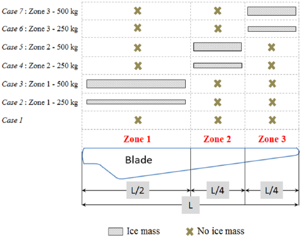
Division of the NREL 5-MW wind turbine blade length into different zones.
Seven different ice mass values are considered in the range of 0–500 kg in each zone, which will generate 343 (equal to
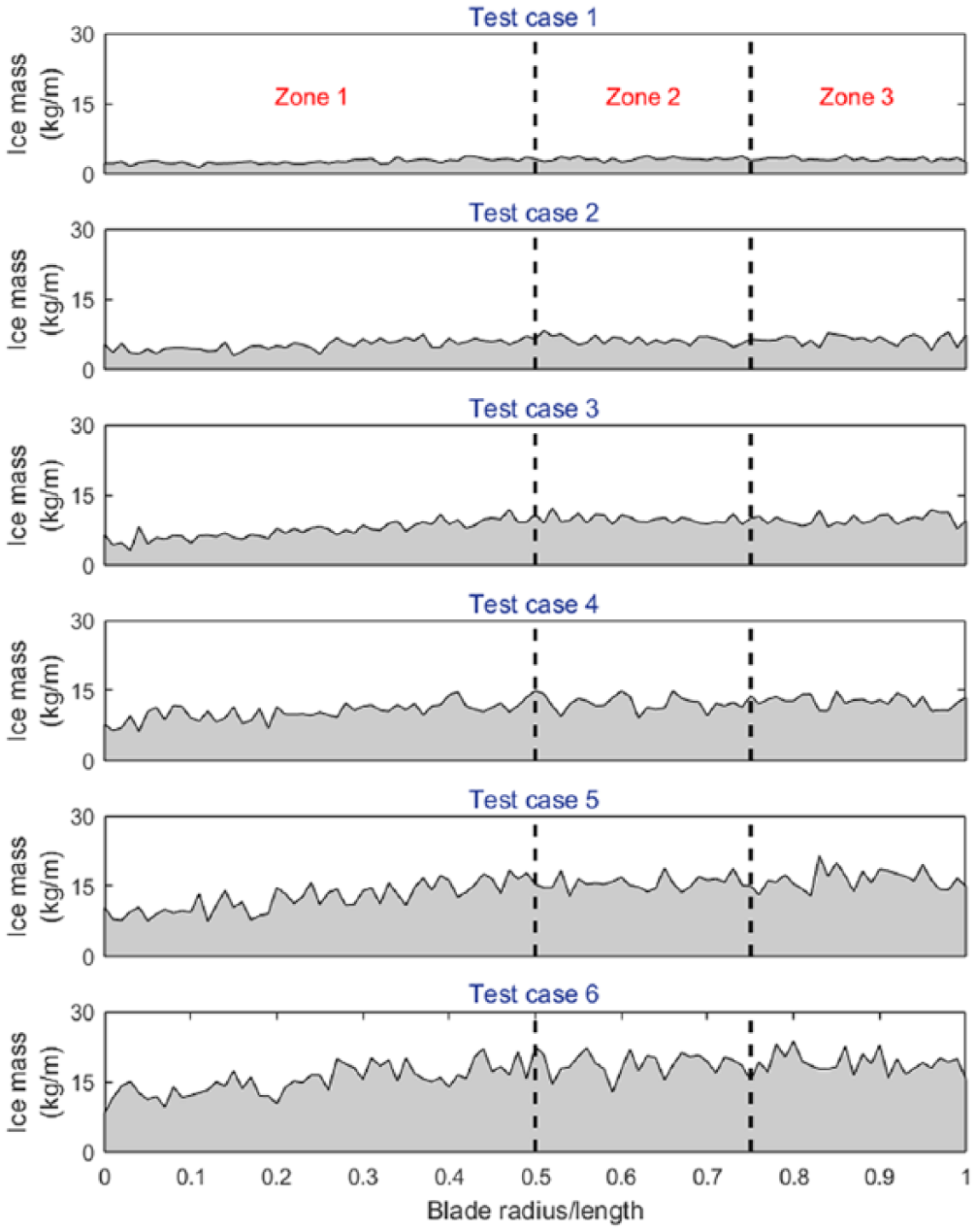
Ice mass distributions considered along the NREL 5-MW wind turbine blade in the six test cases.
Ice masses identified in the 6 test cases: NREL 5 MW wind turbine blade.
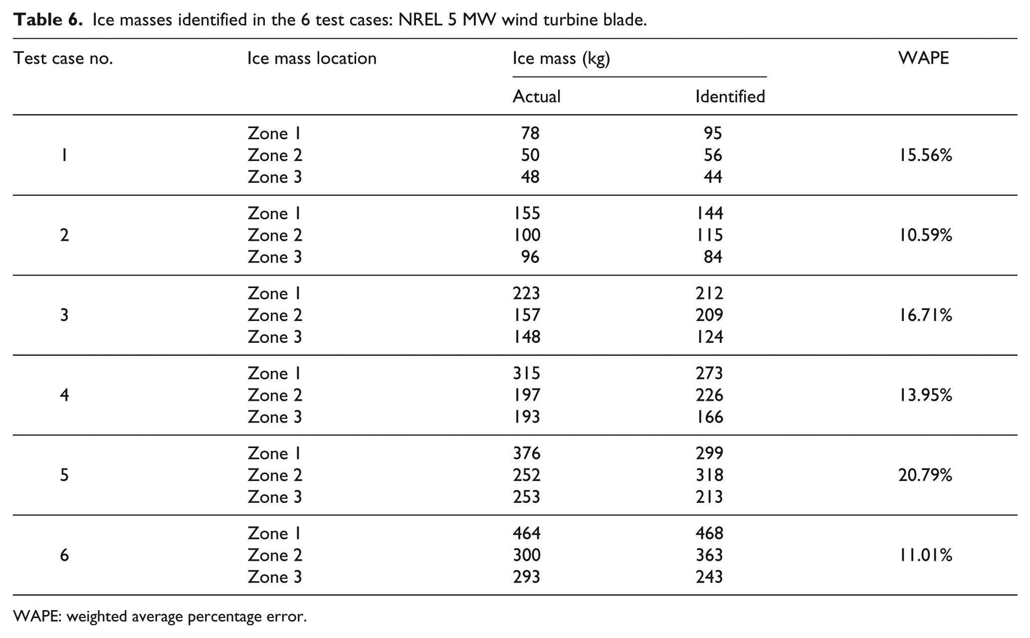
WAPE: weighted average percentage error.
Summary and conclusion
Ice accumulation on a wind turbine blade reduces its natural frequencies differently depending on the location and the quantity of ice mass. In this work, a detection technique is proposed to identify ice masses on a blade based on its first few natural frequencies. The proposed technique is initially demonstrated on a small 1-kW wind turbine blade experimental setup. Experimental modal analyses are carried out on that blade to determine the sensitivities of its natural frequencies to the quantity of ice mass and its location on the blade. An explicit relation to the natural frequencies of the blade is defined in terms of the location and quantity of ice masses using those sensitivities. Later, a data set of natural frequencies of the blade is created using that explicit relation considering different quantities of ice masses at different locations on the blade. An ANN model is trained with this data set where natural frequencies of the iced blade are used as an input and corresponding ice masses at different locations on the blade as an output of the neural network model. ANN approximates a nonlinear relation between these inputs and outputs in the training process. This model is able to approximately identify ice masses with a WAPE value of 17.53% (mean value) in the 18 test cases based on their natural frequencies.
The proposed technique can be applied to detect ice masses on large wind turbines operating in cold climate as it requires only first few natural frequencies of the blade, these frequencies are usually excited by the turbulent wind and can be estimated from the vibration measurements of the blade. The effectiveness of the proposed technique is demonstrated on the NREL 5-MW wind turbine blade where eigenvalue analysis of its FEM model is used to define an explicit relation between its natural frequencies and ice masses on the blade. A neural network model designed using that explicit relation is able to identify ice masses with a mean WAPE value of 14.77% in six test cases. This technique can be used to identify ice masses on a stationary wind turbine, which will allow to optimize and control the de-icing process remotely with the help of information on location and approximate quantities of ice masses present on the blade.
Footnotes
Appendix 1: Values of the polynomial coefficients in equations (2) to (4) for the 1-kW wind turbine blade
Appendix 2: Natural frequencies of the iced 1-kW wind turbine blade identified in the 18 test cases
| Test case no. | Ice masses (g) |
Natural frequencies (Hz) |
||
|---|---|---|---|---|
|
|
Mode 1 | Mode 2 | Mode 3 | |
| 1 | (0, 0, 15) | 9.89 | 45.97 | 125.30 |
| 2 | (0, 0, 30) | 9.69 | 45.71 | 125.10 |
| 3 | (0, 0, 48) | 9.48 | 45.55 | 124.10 |
| 4 | (0, 10, 0) | 10.07 | 45.89 | 124.60 |
| 5 | (0, 25, 20) | 9.73 | 45.41 | 122.40 |
| 6 | (0, 36, 0) | 9.93 | 45.46 | 121.60 |
| 7 | (0, 36, 15) | 9.69 | 45.24 | 121.20 |
| 8 | (10, 0, 30) | 9.67 | 45.42 | 125.10 |
| 9 | (10, 15, 30) | 9.59 | 45.15 | 123.10 |
| 10 | (12, 0, 0) | 10.15 | 45.74 | 125.70 |
| 11 | (12, 0, 26) | 9.75 | 45.42 | 124.80 |
| 12 | (12, 22, 0) | 10.01 | 45.34 | 123.10 |
| 13 | (15, 25, 20) | 9.68 | 44.80 | 121.90 |
| 14 | (25, 0, 0) | 10.13 | 45.37 | 125.60 |
| 15 | (25, 0, 48) | 9.44 | 44.80 | 123.60 |
| 16 | (25, 32, 0) | 9.90 | 44.83 | 121.10 |
| 17 | (25, 32, 48) | 9.26 | 44.17 | 119.50 |
| 18 | (40, 40, 40) | 9.26 | 43.43 | 118.50 |
Appendix 3: Quadratic polynomial fitted between third flapwise natural frequency of the iced NREL 5-MW wind turbine blade (when ice mass is only considered in Zone 3) and respective ice masses used in the Zone 3
Appendix 4: Validation of the approximation used in equation (5) for the NREL 5-MW wind turbine blade natural frequencies with ice masses m 1,m 2,a n d m 3 in Zones 1,2,and 3,respectively
Values of the polynomial coefficients in equations (2) to (4) corresponding to the NREL 5-MW wind turbine blade (with ice masses) natural frequencies are given below
First three flapwise natural frequencies of the blade calculated using an eigenvalue analysis of its FEM model with ice masses (in kg)
From the above table, it is clear that the natural frequencies of iced NREL 5-MW wind turbine blade can be approximately calculated using equation (5) with above polynomial coefficients for given quantities of ice masses
Declaration of conflicting interests
The author(s) declared no potential conflicts of interest with respect to the research, authorship, and/or publication of this article.
Funding
The author(s) disclosed receipt of the following financial support for the research, authorship, and/or publication of this article: This research work is carried out as a part of the project on “Wind power in cold climates” funded by the Swedish Energy Agency, which supports research and development investments in wind power.