Sage Journals: Discover world-class research

Abstract

Analysis of stresses in components of even modestly complex geometries often require the use of finite element analysis (FEA). For testing a large number of design options quickly, FEA can be time consuming and provides more accuracy than required. In this project, a machine learning-based system is developed to provide quick and approximate solutions to stress analysis problems in parametrised compressor disc geometries. Simple mechanics problems were completed preliminarily to test the practicality of machine learning approaches for this application. This included applying instance selection by the $k$ -medoids algorithm to a 2D FEA problem. A parametrised compressor disc geometry was designed and defined by eight dimensions. Stress fields were produced from two superimposed loading schemes: the rotational body force and the force exerted on the disc by the blades 495,338 samples of training data were collected from 4374 FEA simulations. Four networks were trained to predict stresses caused by each loading scheme in order to produce stress fields. The best network was of the structure 9/20/20/2 and used normalised training data. For the geometry tested, it predicted stresses with a root-mean-square error of 1.51%. The code took 0.7 s to run in total, from start-up to completion of a stress plot. The importance of the inputs in the training data set were scored with a feature selection algorithm to aid further optimisation of the system. The low computation time makes this system suitable for the early stages in a design process.

Keywords

Stress analysis machine learning preliminary design finite elements neural networks

Introduction

During the early design stages of a component, it is often necessary to gain an approximate idea of whether a design could withstand the operating stresses before developing it further. A designer frequently desires to test a range of design options of different geometries quickly. Using FEA at each of these design steps is time consuming and provides an unnecessary level of accuracy. Therefore, there is a need for an approach which can quickly provide approximate answers. A machine learning-based system can provide approximate analysis in seconds, where FEA may take a number of hours.¹ Machine learning provides a great advantage when analysing designs of similar geometries. In this study, machine learning has been used to predict the stresses in an axial compressor disc. This problem was considered suitable for a machine learning problem because of the simplicity in parameterising the compressor disc geometry. Additionally, the boundary conditions and loads on a compressor disc are simple to approximate.

The work of Javadi et al.² substitutes the constitutive material model for a neural network incorporated in the finite element programme. The neural network was trained using data representing the stress, strain and displacement response to an applied load. The overall system was effective at estimating the deflection of an end-loaded cantilever formed of nine quadratic quadrilateral elements. The system was trained to find the relationship between stress and strain for non-linear systems. An additional benefit of the model was its ability to incorporate experimental data into the model to more accurately predict the complex behaviours of materials such as soil. The drawback of this approach is the inability to generalise the model for more complex problems.

For irregular 2D geometries, the approach of Nie et al.³ provided a method which was versatile for however less accurate (10.4% error) due to over-simplification of geometries. Cantilever shapes were formed from rectangular elements arranged in a $32 \times 24$ array. Features such as circular holes were modelled by removing rectangular elements in the approximate shape, so the low resolution of the array limited the accuracy. The usage of the array structure for all simulations is required in order to use a convolutional neural network (CNN). The benefit of using the CNN is that the number of input channels remains small even though a large range of shapes can be input. Thus, Nie’s method allowed stress prediction for any 2D cantilever which could be formed of rectangular elements with five input arrays: shape, loads in $x$ and $y$ and boundary conditions in $x$ and $y$ . The use of graph neural networks (GNNs) in producing surrogate FEA models has not been explored extensively. They have been found to improve upon the performance of other surrogate models⁴ by avoiding the errors incurred by CNNs when approximating geometries as pixel grids.⁵ One drawback found in GNNs compared to other NN approaches in the is the increased size and processing of training data, since the required training data includes nodes, elements and edges.

Physics informed neural networks (PINNs) have been found to help reduce the required training data in simple geometries.⁶ However, the improvements to performance and accuracy from physics informing have only been found in nonlinear elastoplasticity.⁷

The complex geometries of aortas were analysed using a machine learning-based process by Liang et al.¹ This was achieved by meshing each aorta by mapping it from a uniform rectangular grid, allowing convolution operations to be used. Before predicting stresses from the shape and internal pressure of the aorta, the input shape data was passed into a shape encoder. The shape encoding process used principal component analysis to represent the 15,000 inputs (5000 nodes located in 3D space) with three scalar values. The stress output was decoded from 64 values up to 15,000 values across the aortic wall.

Madani et al.⁸ approximated stress analysis of artery walls using five different neural networks. The FEA model that data was drawn from analysed 2D cross-sections and simplified blocked arteries into ideal shapes. In general, the networks were trained to predict the maximum von Mises stress and its position in the cross-section. Two of the networks received a set of parameters as inputs and three received an arterial image input for convolutional operations. Some networks also predicted other intermediary outputs, such as heatmaps and prediction of the parameters from an image input. The most accurate von Mises stress prediction (9.86% error) came from mapping the parameters to the stress directly.

Overall, the literature provided examples of machine learning applied to 2D FEA problems and 3D problems which could be solved in a 2D space. CNNs have produced accurate surrogate models for thin 3D geometries which are mappable to a 2D rectangular grid. If a stress field output is required, a truly 3D problem will require significantly more data than a 2D problem. However, if calculating a single maximum stress value and its location from parameters, as carried out by Madani et al.,⁸ 3D problems are feasible for problems which can be defined in a reasonable number of parameters.

Machine learning approaches for mechanical problems

Dimensionality

It was expected that the training data set for the final model would be very large due the large number of inputs. Such data sets are susceptible to the ‘curse of dimensionality’. This refers to problems which arise when training data has high number of dimensions. In order to collect a reasonable amount of data for all combinations of input variables in a high-dimensional feature space, an excessive amount of training data is required. This leads to the opposing problems of having a considerable number of samples or having sparse data in each dimension. Another problem is that the Euclidean distances between all samples in high-dimensional space have significantly less variance. This is problematic for clustering algorithms which attempt to group similar samples to create dissimilar groups. Feature importance techniques (further explained in Section 5.3.2) can help in the process of reducing dimensionality. Inputs with lower importance scores can be removed without significantly impacting the accuracy of predictions.

Minimum redundancy maximum relevance algorithm

Dimensionality reduction is an effective solution to the curse of dimensionality in many regression applications. In this project, dimensionality reduction through mininum-redundancy-maximum-relevance (mRMR) has been explored. mRMR is a feature selection process which ranks input variables by importance. In MATLAB, mRMR is applied through the algorithm proposed by Peng et al.⁹ where starting from a feature set $Ω$ (the input variables), the objective is to find an optimal feature set $S$ . The optimal feature set is one which maximises the relevance $D$ of the set with respect to the target class $c$ (output variable) and minimises the redundancy $R$ of features with respect to each other. The relevance and redundancy are computed using the mutual information $I$ of pairs of variables as a measure of their dependence. For two discrete random variables $x$ and $y$ , the mutual information is given in equation (1) as a function of their probability mass functions, $p (x)$ and $p (y),$ and joint probability mass function $p (x, y)$ .

I (x, y) = \sum_{x} \sum_{y} p (x, y) \log (\frac{p (x, y)}{p (x) p (y)})

(1)

The relevance of the optimal feature set $D (S, c)$ with respect to the target class $c$ is given in equation (2) where $x_{i}$ is a single feature and $| S |$ is the number of features in the set $S$ . The redundancy $R (S)$ of the optimal set is given in equation (3). To find the optimal set, one must maximise $D - R$ .

D (S, c) = \frac{1}{| S |} \sum_{x_{i} \in S} I (x_{i}, c)

(2)

R (S) = \frac{1}{{| S |}^{2}} \sum_{x_{i}, x_{j} \in S} I (x_{i}, x_{j})

(3)

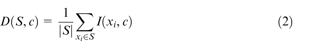
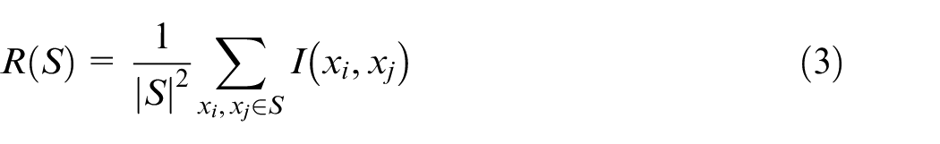
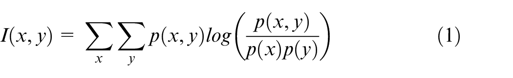
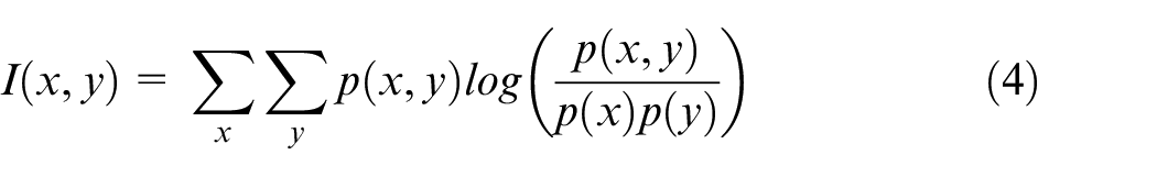
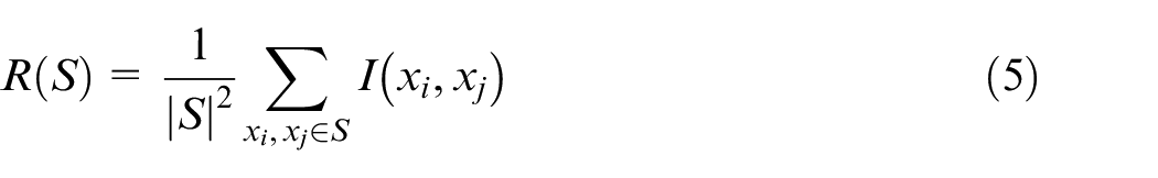
In order to rank features by importance, the relevance and redundancy of each feature is calculated using equations (4) and (5). The ratio $D_{x} / R_{x}$ for each feature is used as a score.

I (x, y) = \sum_{x} \sum_{y} p (x, y) \log (\frac{p (x, y)}{p (x) p (y)})

(4)

R (S) = \frac{1}{{| S |}^{2}} \sum_{x_{i}, x_{j} \in S} I (x_{i}, x_{j})

(5)

Instance selection algorithms

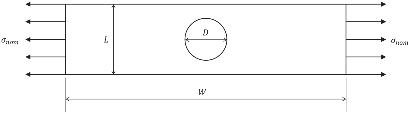
Instance selection aims to reduce the size of a training data set to a smaller representative set with minimal increase in training error. Many efforts have been made to apply clustering algorithms to instance selection, however these have mainly been focused on classification.¹⁰ Rodríguez-Fdez et al.¹¹ proposed an instance selection algorithm composed of three modules which begun with a $k$ -means clustering algorithm. Thus, a similar method was attempted to reduce the training data from a simple 2D stress problem. The problem is defined in Figure 1 where a plate with a hole is under uniaxial tension from a distributed load. The depth of the plate is unity.

Figure 1.

Plate geometry and loads.

The neural network trained for this problem used a structure of (6/12/12/1). The stress at a location ( $x, y$ ) in this problem is affected by six variables [ $L$ , $W$ , $D$ , $σ_{nom}$ , $x$ , $y$ ], which were inputs of a neural network. The output of the network is normal stress in the x-direction, $σ_{xx}$ . Two hidden layers of 12 nodes were used. In the example presented in this paper, training data was compiled from 31 FEA simulations conducted at 31 different values of $D$ . Each simulation consisted of approximately 6000 nodes, the locations of which provided values for the $x$ and $y$ inputs. For elastic examples, the relationship between $σ_{nom}$ and $σ_{xx}$ is linear, so $σ_{xx}$ may be predicted accurately without the use of a neural network. Thus, the value of $σ_{nom}$ was held at $100 MPa$ in the training data. The values of L and W were also held constant in this example. Values of $D$ varied in the range of 0.2 $L$ to 0.8 $L$ . The network accurately mapped the stress distribution including in the areas around the hole with a Root Mean Standard Error (RMSE) of $1.42 Pa$ , shown Figure 2(b).

Figure 2.

Predicted distributions of $σ_{xx}$ calculated by: (a) FEA and (b) a NN trained on the complete FEA data set.

To reduce the amount of redundant training data, a $k$ -medoids clustering algorithm was applied to the data. Similarly, to the more commonly used $k$ -means clustering, the algorithm partitions $n$ samples into $k$ sets (clusters). $k$ -medoids differs in that the centroid of each cluster is a data point chosen from the original set and not an average. One advantage of $k$ -medoids is that it is less sensitive than $k$ -means to outliers. The optimal solution minimises within-cluster variance, however computational methods typically use greedy algorithms, such as partitioning around medoids (PAM), to optimise at a local level.¹² Thus, several iterations may be required to get close to the optimum clustering.

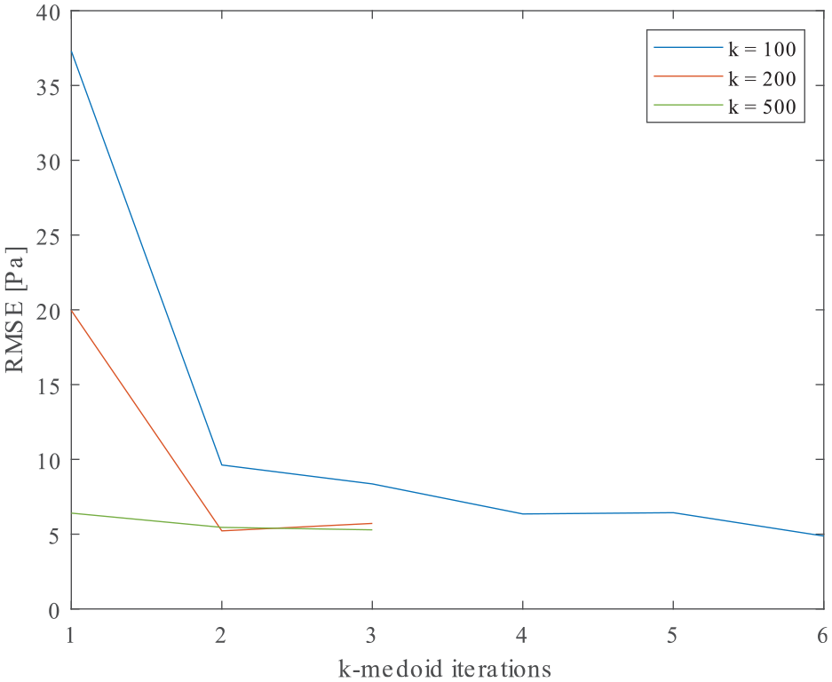
In this application, it was sought to reduce the number of data points in areas of low stress variation. Stress concentrations around the hole would require more samples for accurate regression. The simulations were repeated with $k$ -medoids clustering applied to the finite element results prior to compiling the data set. Values of $k$ of 100, 200 and 500 samples were trialled. Three variables were used for clustering: $x$ and $y$ position and $σ_{xx}$ . The root mean squared errors of stress fields predicted using different values of $k$ are displayed in Figure 3. As expected, using more samples and more iterations of $k$ -medoids led to more accurate results. All models appeared to converge at a minimum RSME of approximately $5 Pa$ .

Figure 3.

RMSE of NNs trained on downsampled data sets.

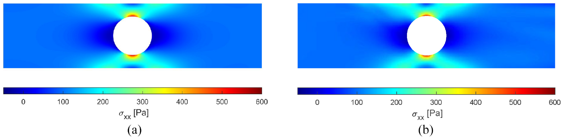
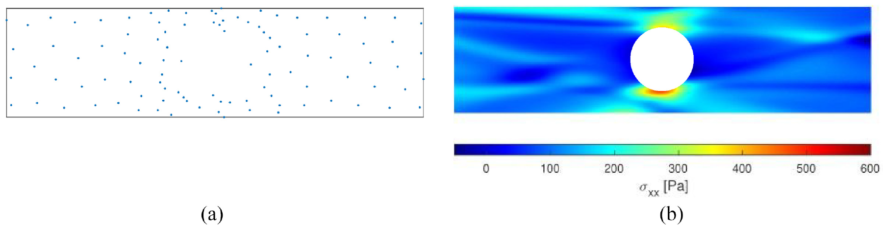
With low numbers of clusters and iterations, centroids were distributed highly asymmetrically and stress distributions appeared skewed. Figure 4(a) displays an arrangement of 100 centroids after one iteration of $k$ -medoids. Centroids are more densely placed towards the top-right and lower left of the hole despite the true stress field being vertically and horizontally symmetric. The resulting stress field in Figure 4 is very inaccurate and underestimates the maximum stress by 15%. In contrast, the distribution of centroids from six iterations in Figure 5 is closer to being symmetric and results in a more accurate stress field.

Figure 4.

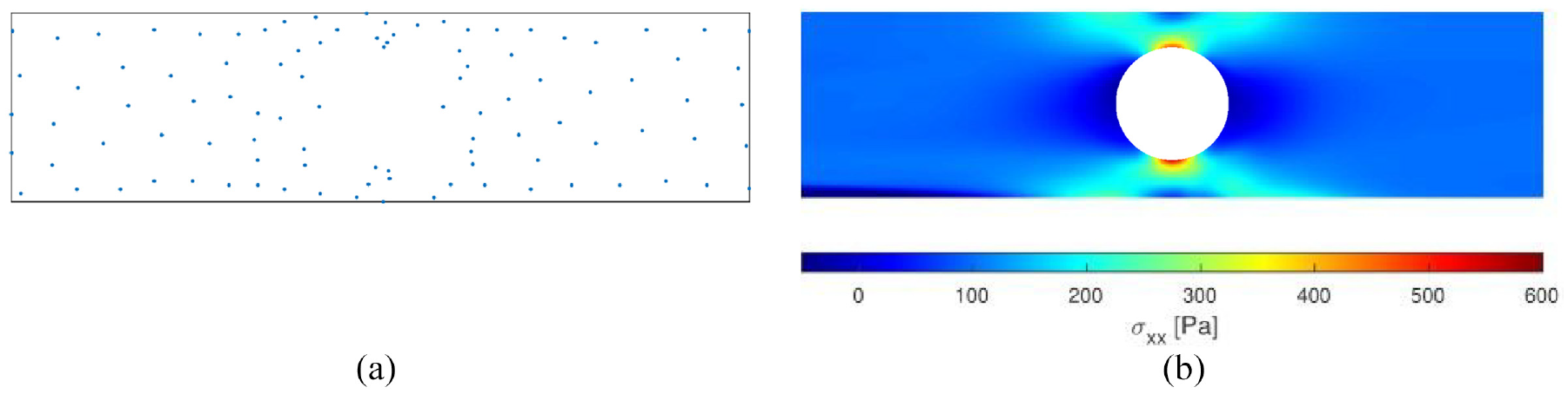
Data sampling and network performance with $k = 100$ and one iteration of $k$ -medoids: (a) centroid locations and(b) predicted distribution of $σ_{xx}$ .

Figure 5.

Data sampling and network performance with k = 100 and six iteration of k-medoids: (a) centroid locations and(b) predicted distribution of $σ_{xx}$ .

Completing four iterations of $k$ -medoids increased the average time per simulation from $1.7 s$ to $6.6 s$ . The PAM algorithm is of computational complexity $O (n^{2} k^{2})$ . For a compressor disc model, the results of the mesh refinement study in Section ‘Finite element model’ indicate that fewer than 200 nodes are required. This is a factor of 30 fewer than the number of nodes used in finite element analyses. It was also noted that clustering using three variables was significantly slower than using two variables. Additionally, clustering algorithms are ineffective in high dimensional space due to distance functions computing smaller differences in distance between samples. These problems can arise at as few as 10–15 dimensions.¹³ The results from this study were promising for the compressor disc model, however, they indicate that the dimensionality of the model must be reduced through feature selection before the $k$ -medoids algorithm can be applied.

Compressor disc model

Model geometry

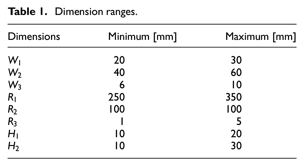
A simplified model of a compressor disc was devised to define the stress analysis problem. First, loading schemes and boundary conditions were identified. Then the geometry was parametrised so that FEA simulations in Abaqus could be automated. The training data set was built using FEA data from automated simulations using different combinations of parameters. The simplified axial compressor profile in Figure 6 is based on previously used models for fatigue analysis in compressor discs.^14,15 Table 1 lists a range of example values that were modelled.

Figure 6.

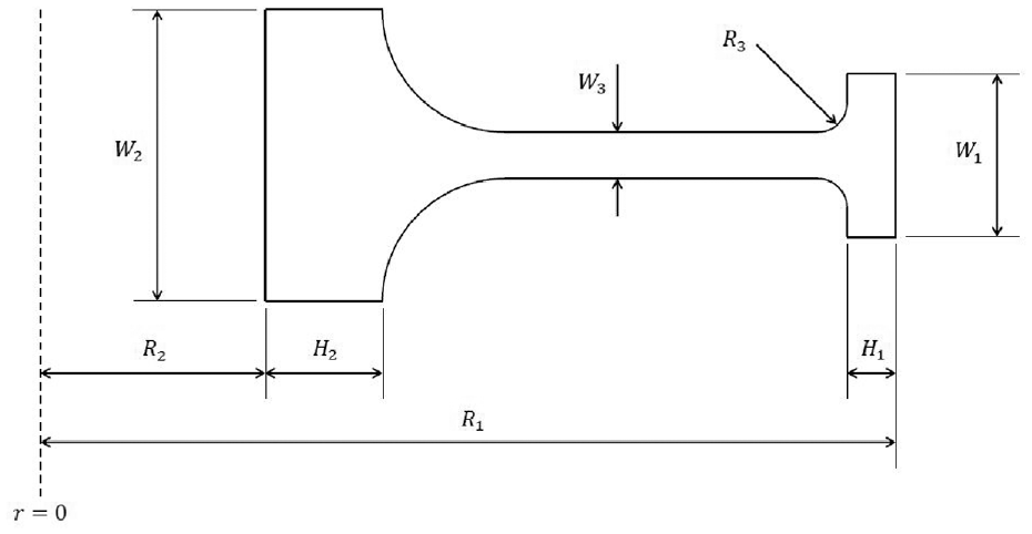
Compressor disc profile dimensions.

Table 1.

Dimension ranges.

Dimensions	Minimum [mm]	Maximum [mm]
$W_{1}$	20	30
$W_{2}$	40	60
$W_{3}$	6	10
$R_{1}$	250	350
$R_{2}$	100	100
$R_{3}$	1	5
$H_{1}$	10	20
$H_{2}$	10	30

An axisymmetric model was chosen to simplify the problem to 2D. This approximation is more suitable for an assembly which uses circumferentially orientated dovetail joints between the disc and blades. Although the local stress concentrations produced at axially orientated dovetails are not axisymmetric, the local stress effects are assumed to diminish away from the joints by Saint-Venant’s principle to a degree that they can be ignored for first-pass stress analysis of the overall disc geometry.

Finite Element Model

Applying the previously mentioned assumptions yields the model set up in Figure 7. The model considers the distributed body-force due to disc rotation together with the radial force due to the blades, which is modelled as a negative pressure on the outer rim. These loads are modelled separately for each geometry so that they may be adjusted independently in the final machine learning-based system.

Figure 7.

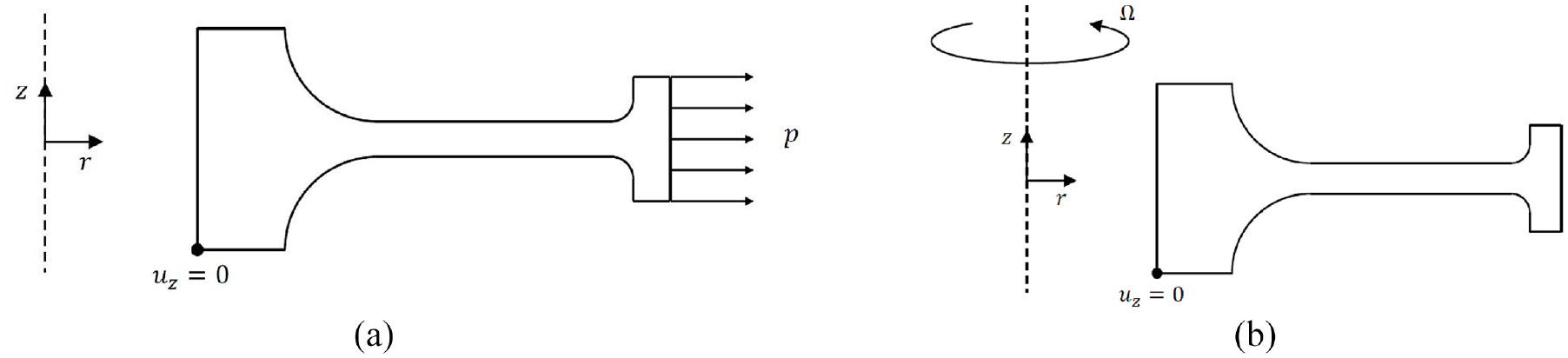
Loading schemes of the compressor disc: (a) radial load from blades and (b) rotational body force.

To reduce both computation times and the size of the output data, the minimum required mesh refinement was determined using a mesh refinement study. The model used for the study had dimensions in the middle of each range in Table 1. A study was performed separately for both loading schemes. The study showed that for this model, a mesh refinement which generated 129 four-node reduced-integration axisymmetric solid elements (CAX4R) was required for the maximum tangential stresses to be within 10% of the converged solutions. This level of mesh refinement was used to build the training data set. Results from the neural network were later compared to FEA results from a refined mesh of 7537 elements, which provided results within 1% of the converged solutions. The stress from the rotational body force was significantly less mesh dependent than the stress from the blades. The stress fields due to the blades (discussed below in Section Results) show greater stress concentration at internal corners. The high mesh dependency of the stress from the blades is a result of stress concentration features only being resolved at higher mesh refinements than the rest of the stress field.

Parameter selection

As seen in Table 1, the geometry of the profile of the compressor disc is defined by eight dimensions. Additionally, the rotational body force is dependent on the angular velocity $Ω$ and the radial load on the rim is additionally dependent on the characteristics of the blades. Some parameters were non-dimensionalised to minimise the number of inputs.

Rotational body force scaling

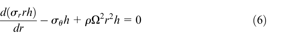
Analysing the loads on a volume element of a thin rotating disc of thickness $h (r)$ results in the equilibrium equation in equation (6). The strains $ε_{r}$ and $ε_{θ}$ can be expressed in terms of stresses leading to equation (7) for a disc with uniform temperature. These equations are only valid for plane stress conditions which are not present at all points on the modelled geometry, however plane strain conditions can be represented by adjusting the elastic constants. The stresses of a scaled version of the disc geometry can be found by non-dimensionalising the two equations with $r^{*} = r / R_{1}$ and $h^{*} = h / R_{1}$ . The non-dimensionalised compatibility equation shows that the ratio of $σ_{r}$ to $σ_{θ}$ is dependent only on $r^{*}$ and not $R_{1}$ . The non-dimensionalised equilibrium equation shows that the combination of stresses in equation (6) scale with $R_{1}^{2}$ . This analysis shows that the stresses due to the body force scale with $R_{1}^{2}$ and $ρ$ . In this project, all analysis has been completed at $ρ = 7872 kg / m^{3}$ .

\frac{d (σ_{r} rh)}{d r} - σ_{θ} h + ρ Ω^{2} r^{2} h = 0

(6)

\frac{d}{dr} (\frac{σ_{θ}}{E}) - \frac{d}{dr} (ν \frac{σ_{r}}{E}) - \frac{(1 + ν)}{rE} (σ_{r} - σ_{θ}) = 0

(7)

Radial load scaling

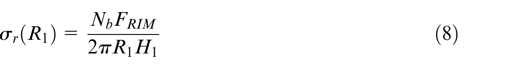
The pressure load applied on the rim is expressed in terms of the resultant radial stress in equation (8) where $F_{RIM}$ is the centripetal force required to keep one blade attached. There are $N_{b}$ blades of mass $m_{b}$ and the centre of mass of each blade is located at a distance $R_{m}$ from the axis of rotation. Since this stress distribution is caused by an applied load, it is evidently simple to scale the stress distribution with each term in the applied pressure equation, including $R_{1}$ .

σ_{r} (R_{1}) = \frac{N_{b} F_{RIM}}{2 π R_{1} H_{1}}

(8)

F_{RIM} = m_{b} R_{m} Ω^{2}

(9)

Model parameters

Since stresses from the body force and the blade load scale with the model size, stress distributions can be calculated from the FEA results of a scale model. Therefore, dimensions of the model can be normalised with respect to a chosen dimension, which reduces the number of dimensional parameters by one. Normalisation was accomplished by dividing all dimensions by $R_{2}$ . Since both stress distributions are proportional to $Ω^{2}$ so the angular velocity does not require an input. In addition to the dimensions, the $r$ and $z$ locations of each node were also inputs, resulting in the following nine input parameters [ $w_{1}$ , $w_{2}$ , $w_{1}$ , $r_{1}$ , $r_{3}$ , $h_{1}$ , $h_{2}$ , $r$ , $z$ ]. As previously discussed, the loads from the rotational body force and blades may be considered independent. The overall stress in a blisk can be found from superimposing the stress components from each of these loads. The two outputs of the network are the tangential stresses $σ_{θ}$ produced by each load [ $σ_{θ, blades}, σ_{θ, body}$ ] at the input location ( $r, z$ ).

Data collection

Training data was collected from FEA simulations in the Abaqus software suite. In each simulation, the position and tangential stress $σ_{θ}$ was recorded at each integration point. In the application of a compressor disc, fatigue should be considered to be an important failure mechanism. When considering Mode I fatigue crack growth, principal stresses would be most appropriate to consider. However, principal stresses from the two loading schemes cannot be simply superimposed because the principal stress directions will differ.

A Python script was used in conjunction with Abaqus to complete stress simulations at three values of each of the seven parameters. The applied loads were $1 rad / s$ of rotational speed or $1 Pa$ of pressure on the outer face to simplify post-process scaling. Three values were used in simulations for each normalised dimension – the minimum, maximum and midpoint of the range. Since the rotational body force and radial blade load were simulated separately, a total of $2 \times 3^{7} = 4374$ simulations were completed, amounting to a total time of approximately 19 h on a computer with 4 CPU cores of 3.4 GHz speed and 8 GB of RAM.

Machine learning model

In many stress analysis applications, the information of most importance is a maximum stress value and its location. An approach which calculated only this information would have been suitable with one loading scheme. However, with two independently adjustable loading schemes, the total stress at any point must be calculated by superimposing the stress fields. The overall maximum stress may not be located at the maxima of either of the separate stress fields. Thus, stresses must be computed at a range of locations and the machine learning-based system becomes a substitute for FEA.

Data pre-processing

Results from the simulations were read into MATLAB and compiled into one data set with 495,338 samples with nine inputs and two outputs. Although the inputs were varied in orders of magnitude, normalisation of inputs, which often scales the values of inputs into a range [0, 1], was not required for regression because any necessary rescaling could be accomplished with the weights and biases. Since the outputs varied greatly with the rotational stress being approximately four orders of magnitude greater than the stress from the blades, a second version of the training set was produced with normalised output variables. Values of each output in the training data were mapped to the range [0, 1]. Normalising data to the same scale speeds up the training of a feed-forward network.¹⁶

Neural network designs

As previously stated, an initial network was designed to follow the assumption that two hidden layers of $2 n + 1$ nodes for $n$ inputs would be sufficient.¹⁷ Thus a 9/20/20/2 network was trained. Instead of training by conventional gradient descent, the Levenberg-Marquardt backpropagation method was used. The Levenberg-Marquardt method¹⁸ is an error minimising technique which interpolates between gradient descent and Newton methods. As the MSE is reduced, the method is shifted towards Newton methods which are faster near the minimum. The Levenberg-Marquardt backpropagation uses the strengths of both constituent methods to converge faster.

The data was split into training, validation and test data sets in a 70:15:15 ratio. Training was stopped if a network had not converged after being trained for at least 1000 epochs and for 1 h. While training with the original training data set, convergence was not achieved within these conditions so the training was paused. To check whether a network of a smaller capacity would suffice, a 9/10/10/2 network was also trained. Similarly, convergence was not achieved in a reasonable time using the original data set, however the network passed the validation criteria within 677 epochs using the normalised data set.

Data post-processing

Values of the tangential stress were produced by selecting values for the disc profile dimensions, angular velocity $Ω$ , $N_{b}$ , $m_{b}$ and $R_{m}$ . As mentioned in Section ‘Compressor disc model’, the stress from the body force was scaled by the $R_{2}^{2} Ω^{2}$ and the stress from the blades was scaled by the terms in equation (6) before the stresses were superimposed.

In order to produce a stress distribution, the stress had to be plotted queried at several points. When the dimensions of the model being queried belonged to the training set, a simple approach was to query at the same points stress had been measured from. The MATLAB function ‘griddata’ was used to linearly interpolate between integration points in a manner similar to that for FEA postprocessor. Originally, queries were made at an evenly spaced grid of points where some were located outside the disc profile. This approach to querying increased the error between the predicted stress field and the stress field produced by the corresponding FEA data in the training data set. So, points were initially selected only within the bounds of the geometry. This result is further discussed in Section ‘Sampling accuracy’.

Results and discussion

Results

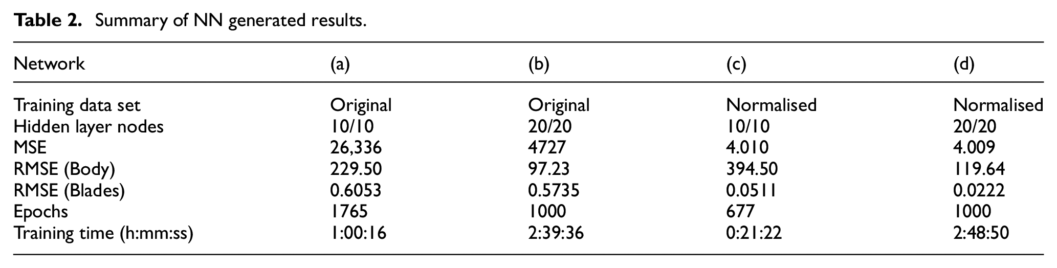
Table 2 summarises the results of the four networks detailed in Section ‘Neural network designs’, which have been labelled networks (a) – (d). Although all networks were trained to minimise MSE, the results cannot be used to compare networks which have used different training sets. An RMSE for each output has been provided separately for the networks (a) and (b). For networks (c) and (d), the RMSE values have been scaled to reverse the scaling which was used to normalise the data set, so that RMSE values are comparable across data sets. The RMSEs show that the normalised data sets allowed networks (c) and (d) to optimise themselves to map to each output more equally. The normalised data also allowed network (c) to converge within the stopping criteria for training.

Table 2.

Summary of NN generated results.

Network	(a)	(b)	(c)	(d)
Training data set	Original	Original	Normalised	Normalised
Hidden layer nodes	10/10	20/20	10/10	20/20
MSE	26,336	4727	4.010	4.009
RMSE (Body)	229.50	97.23	394.50	119.64
RMSE (Blades)	0.6053	0.5735	0.0511	0.0222
Epochs	1765	1000	677	1000
Training time (h:mm:ss)	1:00:16	2:39:36	0:21:22	2:48:50

In order to analyse the distribution of stresses more closely, a geometry with one set of dimensions has been selected for analysis. This geometry has dimensions at the midpoint of their range specified in Table 1 and will be referred to as the ‘average disc geometry’. The stress plot in Figure 8(a) shows the total circumferential stress in the average disc profile from values calculated by FEA. 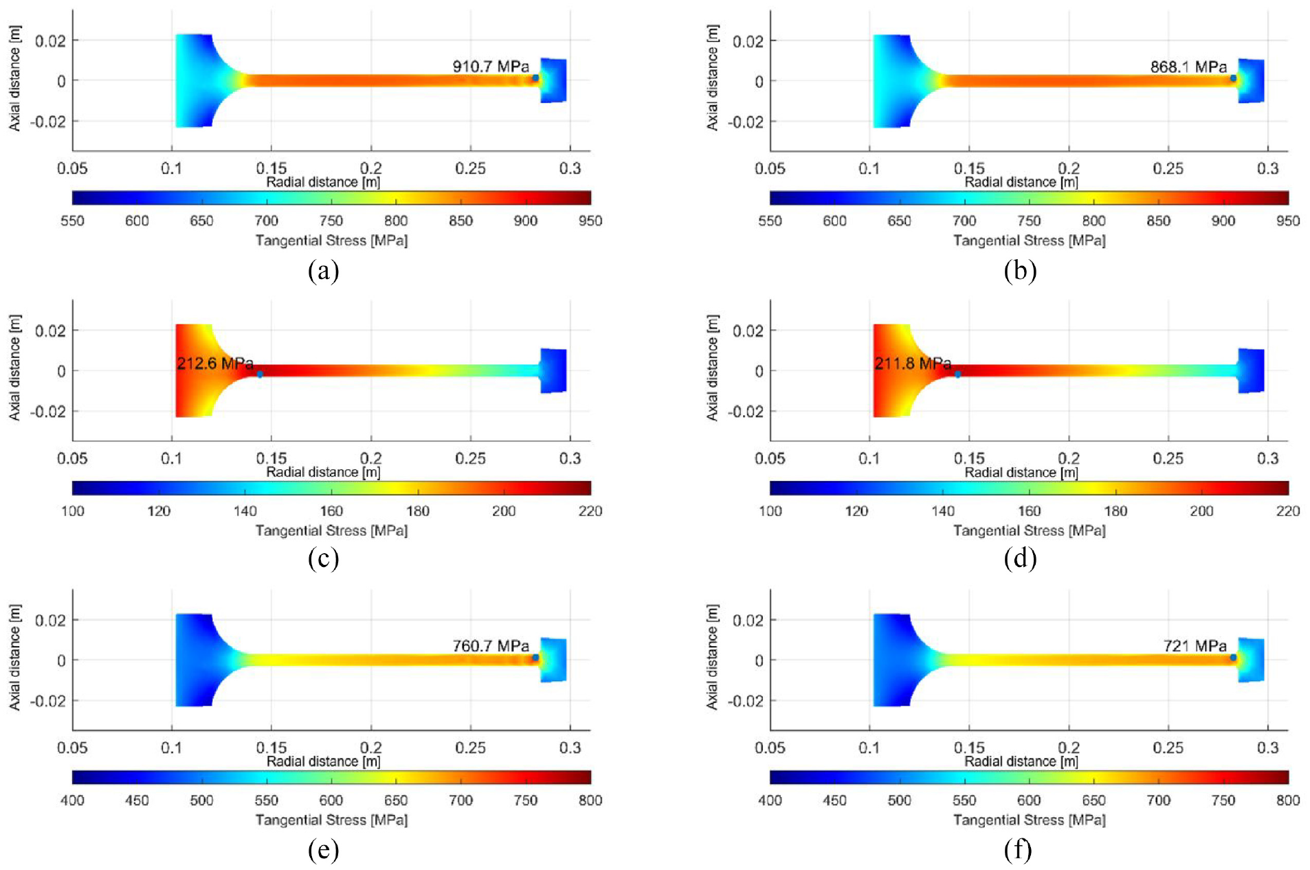The stress from the blades and rotational body force have been scaled and superimposed using the example parameters: $Ω = 800 rad / s$ , $N_{b} = 52$ , $m_{b} = 0.047 kg$ and $R_{m} = 0.35 m$ . Figure 8(c) and (e) show the FEA solutions for stress fields from each loading scheme.

Figure 8.

Tangential stresses computed by FEA and the neural network model: (a) total tangential stress, FEA, (b) total tangential stress, NN, (c) total tangential due to rotation, FEA, (d) total tangential due to rotation, NN, (e) total tangential due to blades, FEA and (f) total tangential due to blades, NN.

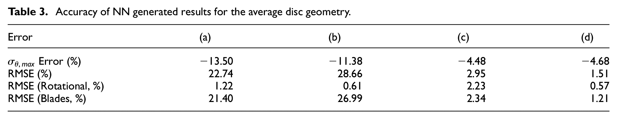
The four networks detailed in Section 10 were first tested with this geometry. The input dimensions were part of the training data set, meaning that an overfitted network would be able to map the values accurately. However, underfitting was suspected of being more likely than overfitting due to difficulty in reaching convergence in training and the large quantity of data. Results are recorded in Table 3. The circumferential stresses along the radius at the midplane $(y = 0$ ) are plotted in Figures 9 and 10 for each loading scheme.

Table 3.

Accuracy of NN generated results for the average disc geometry.

Error	(a)	(b)	(c)	(d)
$σ_{θ, \max}$ Error (%)	−13.50	−11.38	−4.48	−4.68
RMSE (%)	22.74	28.66	2.95	1.51
RMSE (Rotational, %)	1.22	0.61	2.23	0.57
RMSE (Blades, %)	21.40	26.99	2.34	1.21

Figure 9.

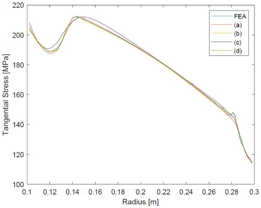
Stress across the disc midplane due to rotational loads.

Figure 10.

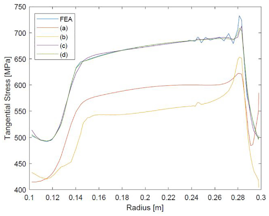
Stress across the disc midplane due to radial loads from the blades.

Accuracy

It is clear from the overall stress plots that all networks were accurate in regions of gradual stress variation. Maximum stresses were calculated with mixed accuracy and all predictions were underestimates. In the stress fields of some geometries not displayed here, the maximum stress was located nearer to the bore where the stress varied more gradually. In these cases, the maximum stress prediction was more accurate.

Rotational body force

The stress from the body force was predicted very accurately from all networks and is reflected in the low error values. This is likely due to the mostly linear nature of stress variation radially, with only a minor outlying stress concentration at $r = 0.28 m$ (where the disc widens at the rim). The regions where the disc thickness is changing are clear from the different gradients. Network (c), which passed the validation criteria before training was paused, appears the least closely matched to the FEA data indicating that the other networks may be overfitted.

Radial load

The midplane stresses from the radial load in Figure 10 show large variation in accuracy between the networks. The networks trained from the original data set are offset from the FEA result by

approximately $80 MPa$ and $120 MPa$ . This is likely due to the stresses being four orders smaller than the rotational stress in the data set. Since the MSE, which is minimised during training, is not normalised, training will favour a variable of greater magnitude. It is notable that network (a) performed better than network (b) despite having fewer nodes. This could be due to the stopping criteria allowing it more training epochs. However, network (a) predicted highly erroneous stresses towards the edge of the rim $r = 300 mm$ . Sharp fluctuations are usually characteristic of overfitted networks however the other regions of output, such as the stress concentration at $r = 280 mm$ , indicate the opposite. Networks (c) and (d) have accurately mapped the stress but have also smoothed minor fluctuations in the FEA data. The oscillations of the FEA data from $r = 240 mm$ are possibly present due to insufficient mesh refinement around the stress concentration. In this stress field the stress concentration is larger and the stress increases over a short distance. Networks (c) and (d) predict a rise in stress at the rim of approximately half of that in FEA data resulting in a 3% error. However, the result of the mesh refinement study and the fluctuations near to the maximum stress, indicate that the error in the FEA data is significantly larger than that of the networks (c) and (d). Although a small error, it highlights a drawback to this approach for stress analysis. Stresses will increase quickly around a stress concentration and a neural network may underestimate these in the manner that it would with statistical outliers. While MSE ensures very large errors will not occur as they are penalised heavily, stress concentrations are usually the points of greatest stress in a design, so utility is wasted if predictions are accurate in all regions but stress concentrations. For geometries with specific features, such as internal corners and holes, a physics guided approach could improve the accuracy of predictions in these regions.

If there were only one loading scheme, a solution to this problem would be to introduce a separate output for the maximum stress in a geometry. This output would only require the seven inputs corresponding to the disc dimensions without needing locations of integration points. With two superimposed loading schemes a maximum stress can be predicted for each scheme which is then added to the stress caused from the other loading scheme at that location. Even with accurate predictions of the maximum stress, inaccuracies will still remain at smaller local stress maxima.

Sampling accuracy

As mentioned in Section ‘Data post-processing’, sampling the stresses at points led to results which differed from the FEA data. It is common practice to not query a network outside of the range of the training data, however the integration points in the training data were located within the edges of the profile. Since stress concentrations are often located on edges, the stress data required extrapolation to the edges. Extrapolation could be done either linearly in MATLAB (similarly to a FEA package) or by querying stresses outside the geometry and interpolating. As seen in Figure 10, the internal corner of the rim is a stress concentration under radial loading. In the mesh refinement study, a relatively large error of 10% was settled upon. This resulted in the mesh in Figure 11(a) being used to produce training data for the average disc geometry. 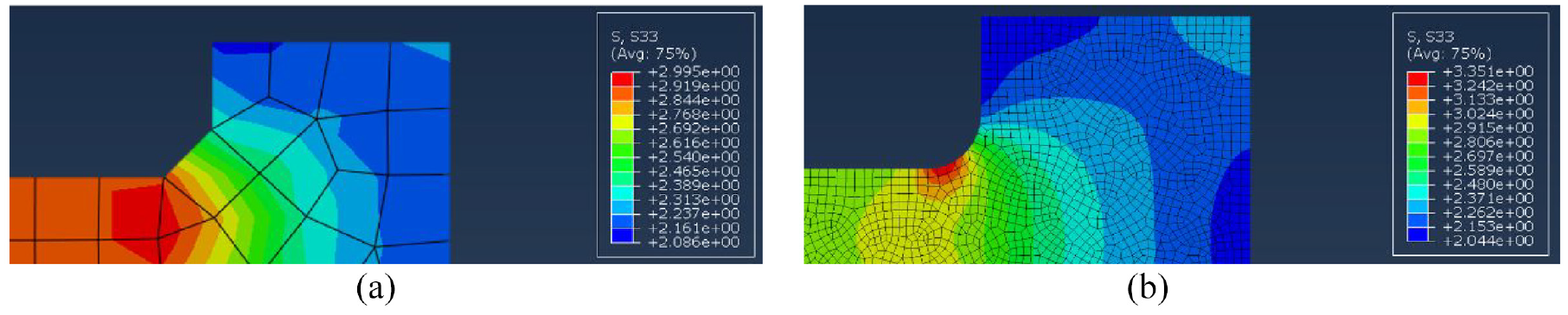From this mesh, no stress concentration effect is visible and Abaqus measured a maximum stress of $2.995 Pa$ under the unscaled radial load ( $1 Pa$ ) at the rim. When results are exported, the maximum stress at any integration point is $3.07 Pa$ . MATLAB’s linear interpolation process computes a maximum stress of $3.074 Pa$ . Figure 11(b) shows a mesh with refinement around the internal corner. The stress concentration at the corner is visible and the maximum tangential stress is $3.351 Pa$ . The error of the $σ_{θ, \max}$ in the in the exported coarse mesh relative to the refined mesh is −7.88% and the RMSE error across the geometry is 3.20%.

Figure 11.

Results of mesh convergence study – tangential stress under a 1 Pa radial load: (a) coarse mesh and (b) refined mesh.

Figure 12(a) displays the FEA data for this study after processing in MATLAB, as well as the predictions from network (d). As expected, the stress results from the neural network in Figure 12(c) did not capture the separate stress concentrations at each corner when using samples from within training data from FEA simulations which themselves did not represent this feature. However, when querying outside of the disc profile, network (d) displayed stress concentrations (Figure 12(d)) similar to those displayed by the refined mesh and predicted a maximum tangential stress of $3.288 Pa$ . This result is closer to the maximum stress of the refined mesh than the prediction when querying within the integration points ( $2.981 Pa$ ) although the MSE to the unrefined FEA solution is increased. The errors incurred by both querying strategies are summarised in Table 4. It was expected that querying outside the integration points increases the RMSE to the coarse FEA result it is trained from. However, it is interesting to note that external querying reduces the RMSE to the refined result. This is a result of the neural network extrapolating more accurately than the typical shape functions and linear extrapolation that a FEA code would use for reduced order CAX4R elements. Linear interpolation is only dependent on the ‘nearest neighbours’ to the location where stress is being evaluated. However, the neural network is trained on all of the data points from all simulations, so it is capable of mapping trends which are present across several simulations This has resulted in a model which remains adequately accurate when extrapolating a short distance outside the integration points.

Figure 12.

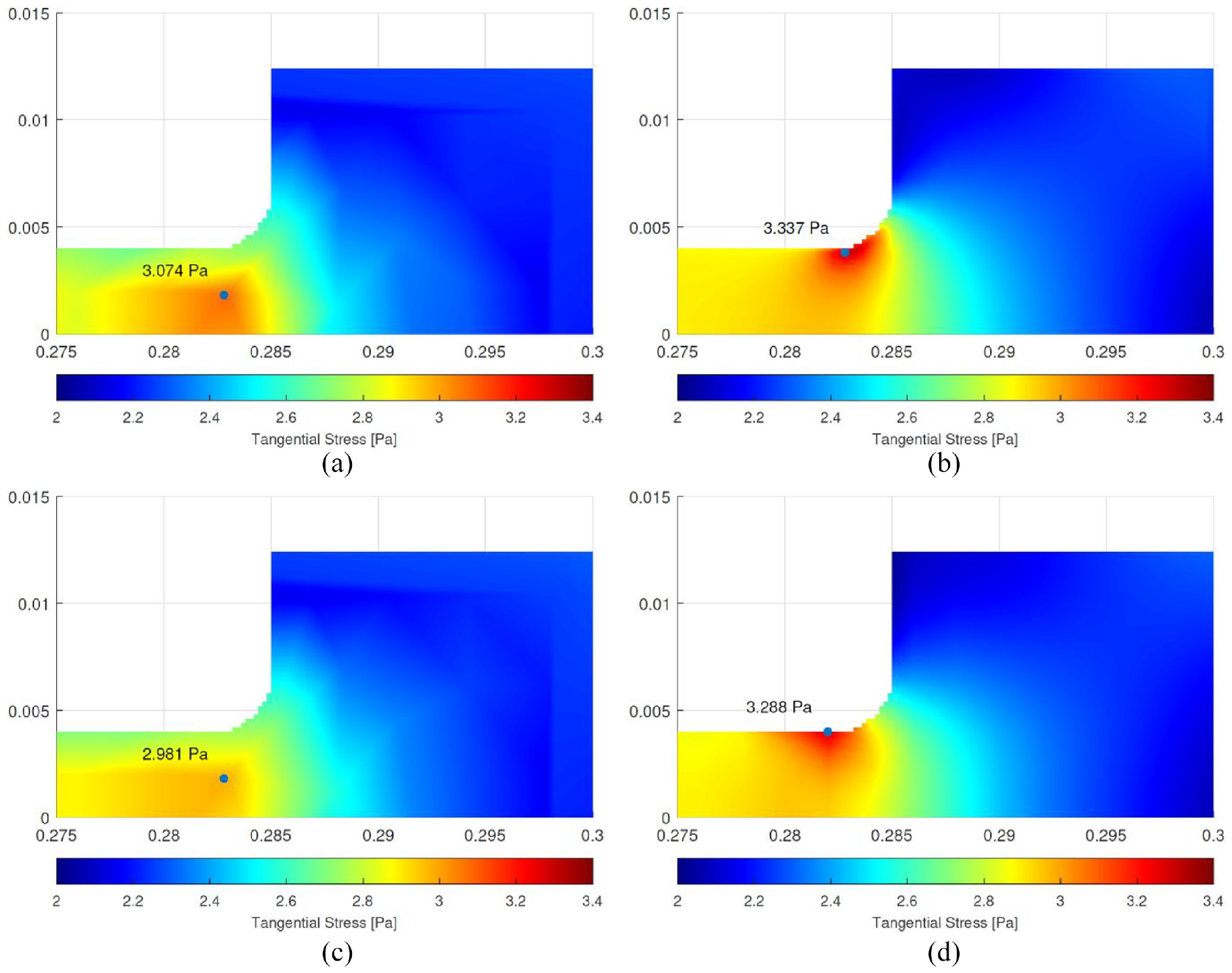
Tangential stress predictions at the rim under a 1 Pa radial load: (a) FEA data from the training data set, (b) FEA data from a refined mesh, (c) NN prediction from queries within the bounds of the integration points and (d) NN prediction from queries outside the bounds of the disc profile.

Table 4.

Errors incurred with querying methods.

Error	Internal querying only (%)	Externalquerying (%)
RMSE to coarse FEA	1.21	4.67
$σ_{θ, \max}$ error to coarse FEA	−3.03	6.96
RMSE to refined FEA	4.84	1.67
$σ_{θ, \max}$ error to refined FEA	−10.67	−1.47

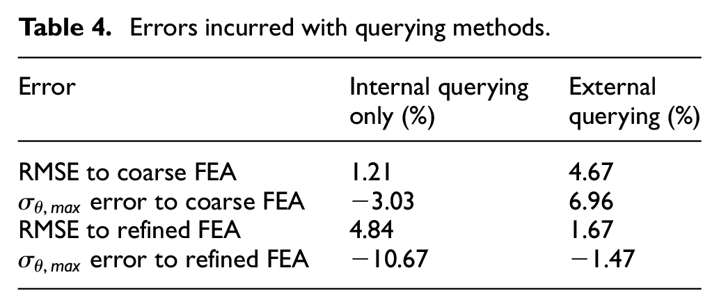
Overall, extrapolation from the integration points is performed more effectively by the NN and the error at the internal corner is reduced to −1.47%. The mean error from this approach is lower than or comparable to typical NN-based FEA surrogate models. Among the models described in Section ‘Introduction’,^3,8 an overall error of approximately 10% is commonplace. An advantage of this method is that the training data meshes are of a lower refinement to the desired output stress field. The different meshes and thus different node locations, between training data geometries allow the NN to compute stresses around the internal corner more accurately than FEA can achieve with a single mesh of similar refinement to the training data. Conversely, this approach would be ineffective at solving a problem where the geometry and node position around stress concentration features are constant across all designs, such as a cantilever beam,² unless mesh controls around the feature are intentionally varied between training meshes.

Computation time

Code profiling

Profiling the code revealed that total time to run the code was highly dependent on the resolution of the grid that queried stresses were interpolated onto. For example, a grid resolution of $1 mm$ resulted in a total time of 0.7 s but a $0.2 mm$ required 2.5 s. This is because the stress field to be plotted is first calculated as a rectangular grid of stress values. Each grid location is then individually checked so it may be discarded if it not inside the disc profile so that the final plot is in the shape of a disc. This high computation results from completing this process using a MATLAB function which checks whether the point is within any specified plotted shape. The computation time could be reduced using geometry-specific code.

Feature importance

If the machine learning-based system were to be streamlined or a similar system were made using less data, it would be beneficial to identify the variables of most importance. The mRMR algorithm explained in Section ‘Minimum redundancy maximum relevance algorithm’ was applied to check the importance of the inputs in predicting each output. Figure 13 displays the predictor importance scores for the stresses from the rotation and blades respectively. 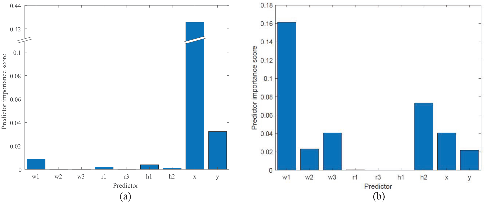Note that $x$ , $y$ and all dimensions are those of the normalised geometry.

Figure 13.

Predictor importance for tangential stress prediction: (a) predictor importance for tangential stress due to rotational load and (b) predictor importance for tangential stress due to blade load.

Figure 13(a) shows that the rotational is most dependent on $x$ and this is reflected in the stress field in Figure 8(c) where there is little variation of stress in $y$ . After the $x$ and $y$ location, $w_{1}$ and $h_{1}$ are the most important parameters which is an expected results as the mass near the rim has a greater effect on stresses than mass at the bore. Figure 13(b) shows a more even spread of importance of variables. The high importance score of $w_{1}$ is due to the pressure load applied on the rim being constant. The appropriate scaling was applied in the post-processing, however a more meaningful importance score could have been gained from scaling with respect to $w_{1}$ in the FEA code.

Across both loading schemes, the least important parameter was $r_{3}$ . Whilst $r_{3}$ may be unimportant in this data set, further investigation should be completed to determine its real effect on stresses. The radius of the internal corner was not modelled well in the FEA simulations and thus the resulting stress concentrations were not modelled accurately. Except for $r_{3}$ , no variable was of very low importance to both stress fields.

Conclusions

Machine learning techniques and their application in stress analysis have been investigated. A literature review has been conducted into existing approaches to solving similar mechanical loading problems using neural networks.

Data pre-processing methods were explored to reduce redundancy in the training data. The data reduction method – instance selection was trialled on the 2D stress analysis problem of a plate with a hole under uniaxial tension. Training data was downsampled using $k$ -medoids to remove points in areas of low stress variation. Downsampling from 6000 nodes to 100 nodes with four iterations of $k$ -medoids resulted in a NRMSE of 0.92%.

A machine learning-based system was then developed for a parameterised compressor disc geometry. The compressor disc was subject to loading from rotational body forces and from a radial force exerted by the blades. Four thousand three hundred and seventy-four FEA simulations were used to collect training data was collected from integration points leading to 495,338 samples. Four networks were trained to predict the two tangential stress from the loading schemes using inputs which represented the compressor discs dimensions and the location queried at. Overall, the network with a 9/20/20/2 structure, which used normalised training data, was most effective at minimising MSE across both loading schemes. For a disc geometry with dimensions which were averaged across the dimensions which were tested, this network produced the most accurate stress field with a NRMSE of 1.51%.

The querying locations on the accuracy of the stress field was also investigated. Query only within the bounds of the integration points of the training data produced a stress field with a NRMSE to the training data of 1.21%. Querying at points which were also outside the bounds resulted in a greater error of 4.84%. Interestingly, using external querying reduced the error to the FEA results of a finer mesh from 4.67% to 1.67%. The error from this approach is lower than the typical NN-based FEA surrogate models of a similar scope, as discussed in Section ‘Sampling accuracy’.

The inputs of the networks were ranked by importance with respect to each output using the minimum redundancy maximum relevance algorithm. It was found that the fillet radius at the disc rim $R_{3}$ was the least significant input. Whilst $R_{3}$ was unimportant in the data, this result was likely worsened by the poor mesh refinement at $R_{3}$ in the FEA models.

Overall, the machine learning-based system appears to serve a specialised role in the design of parameterised parts. The performance advantage of the neural network is greatest for problems which FEA takes longer to solve; however this increases the time required to build a training data set. The accuracy of the networks is this project were adequate. Arguably, the speed of neural network is only of use in an exploratory approach to design. The speed of the system allows results to be updated as inputs are updated by a user making it suitable for an interactive computer program. If slightly less speed is necessary, a user-friendly script/application could be used to interface with a FEA package. In this project, FEA studies took approximately 15 s and only required inputs to be entered into a script. Therefore, the neural network has applications in the initial design stages but is less useful when receiving quick results is less important.

Footnotes

Declaration of conflicting interests

The author(s) declared no potential conflicts of interest with respect to the research, authorship, and/or publication of this article.

Funding

The author(s) received no financial support for the research, authorship, and/or publication of this article.

ORCID iD

David Nowell

References

Liang

Liu

Martin

, et al. A deep learning approach to estimate stress distribution: a fast and accurate surrogate of finite-element analysis. J R Soc Interface 2018; 15(138): 20170844.

Javadi

Tan

Zhang

Neural network for constitutive modelling in finite element analysis. Comput Assist Mech Eng Sci 2003; 10(4): 523–529.

Nie

Jiang

Kara

LB.

Stress field prediction in cantilevered structures using convolutional neural networks. J Comput Inf Sci Eng 2019; 1: 1–16.

Jiang

Chen

NZ.

Graph Neural Networks (GNNs) based accelerated numerical simulation. Eng Appl Artif Intell 2023; 123: 106370.

Gulakala

Markert

Stoffel

Graph Neural Network enhanced finite element modelling. Proc Appl Math Mech 2023; 22(1): 1–6.

Rezaei

Harandi

Moeineddin

, et al. A mixed formulation for physics-informed neural networks as a potential solver for engineering problems in heterogeneous domains: comparison with finite element method. Comput Methods Appl Mech Eng 2022; 401: 115616.

Haghighat

Raissi

Moure

, et al. A physics-informed deep learning framework for inversion and surrogate modeling in solid mechanics. Comput Methods Appl Mech Eng 2021; 379: 113741.

Madani

Bakhaty

Kim

, et al. Bridging finite element and machine learning modeling: stress prediction of arterial walls in atherosclerosis. J Biomech Eng 2019; 141(8): 1–9.

Peng

Long

Ding

Feature selection based on mutual information criteria of max-dependency, max-relevance, and min-redundancy. IEEE Trans Pattern Anal Mach Intell 2005; 27(8): 1226–1238.

10.

Song

Liang

, et al. An efficient instance selection algorithm for k nearest neighbor regression. Neurocomputing 2017; 251: 26–34.

11.

Rodríguez-Fdez

Mucientes

Bugarin

. An instance selection algorithm for regression and its application in variance reduction. In: 2013 IEEE international conference on fuzzy systems (FUZZ-IEEE), Hyderabad, India, 7–10 July 2013, pp. 1–8. New York: IEEE.

12.

Kaufman

Rousseeuw

PJ.

Clustering by means of medoids. Delft: Faculty of Mathematics and Informatics, 1987.

13.

Beyer

Goldstein

Ramakrishnan

, et al. When is ‘nearest neighbor’ meaningful? In: International Conference on Database Theory, Jerusalem, Israel, 1999. Berlin, Heidelberg: Springer, pp. 217–235.

14.

Jagannath

SML

Srinivasan

Gopalakrishnan

, et al. Prediction of fatigue and fracture life of an autofrettaged turbine compressor disc using finite element analysis. In: ASME 2014 Gas Turbine India Conference, New Delhi, India, 15–17 December 2014, pp. 1–8. International Gas Turbine Institute.

15.

Giannella

Citarella

Perrella

, et al. Surface crack modelling in an engine compressor disc. Theor Appl Fract Mech 2019; 103: 102279.

16.

Jayalakshmi

Santhakumaran

Statistical normalization and back propagation for classification. Int J Comput Theory Eng 2011; 3(1): 89–93.

17.

Kůrková

Kolmogorov’s theorem and multilayer neural networks. Neural Netw 1992; 5(3): 501–506.

18.

Levenberg

A method for the solution of certain non-linear problems in least squares. Q Appl Math 1944; 2(2): 164–168.

Application of machine learning for ‘what if?’ stress analysis