Industrial application of a low-cost structural health monitoring system in large-scale airframe tests

Abstract

A small, novel, integrated SHM system has been deployed during full-scale testing of a wing fatigue test for several weeks and a fuselage pressurisation test for several months. Complementary NDE measurement techniques were combined, with inputs from visible and infrared optical sensors, as well as resistance strain gauges. Sensor units were deployed at regions of interest and integrated board computers permitted near real-time data processing. The outputs were full-field measurement datasets from digital image correlation and thermoelastic stress analysis systems. Changes in these datasets in the regions of interest were successfully quantified using orthogonal decomposition and were indicative of changes in the condition of the structure. The results from these case studies demonstrate that this system can be successfully deployed in spatially restricted areas within airframe structures to monitor crack growth. The low cost and small footprint of the system presents the opportunity for installation of arrays of similar sensors for both test and in-service data collection. Near real-time data processing would allow timely reporting to service engineers, informing maintenance or operational decisions.

Introduction

Structural health monitoring (SHM) is an important part of testing and in-service use for engineering structures and components. Damage, such as cracks in metals and delaminations in composites, can be indicated by their growth or the associated change of stress and strain distribution. Early detection of damage allows timely intervention for repair, replacement, or redesign, thereby ensuring the safety of these structures.

Several non-destructive evaluation (NDE) techniques are available to detect such changes in stress and strain, some of these are restricted to laboratory testing, whereas other more mature technologies are used routinely in industrial environments. These techniques can be broadly divided in two groups: point measurement and full-field techniques, where point measurement techniques (e.g. strain gauges) collect data from a single position, and full-field methods use array sensors, such as cameras, and are therefore able to cover a larger region of interest with one sensor.

Digital image correlation (DIC) is a full-field technique which is used to measure displacements between consecutive images of a surface on which a speckle pattern has been applied. Strains can then be calculated from these displacements. DIC has been used for damage detection in laboratory and industrial applications.^1–4 Similarly, infrared (IR) sensors are employed for NDE, with methods including passive and active thermography, and thermoelastic stress analysis (TSA).^5–11

As technology develops, visible and IR sensors are becoming smaller and cheaper. The decrease in size and cost broadens the possibilities of using these imaging sensors for NDE techniques in engineering applications. For example, packaged microbolometers costing £1,000s are an order of magnitude less expensive than photovoltaic detectors (£10,000s), but have been shown to have sufficiently high sensitivities to be used for damage detection.^9,12–16 Further developments have resulted in centimetre size imaging sensors which cost on the order of £100s, such as the PiCam (Sony IMX219 8-Megapixel Sensor) and the Lepton 3 (FLIR). The potential of these small sensors for condition monitoring has begun to be explored, for example by Eichhorn et al. ¹⁷ using the imaging sensors for DIC, and Middleton et al. ⁹ and Paiva et al. ¹⁸ using the infrared sensors for TSA.

As a large volume of data is collected when using full-field NDE techniques, approaches to data storage and processing must also be considered, particularly when tests can last months or years. Real-time processing of data is of particular importance for monitoring the progress of the test, where timely intervention is necessary to either halt a test and carry out further inspection or repair, or to inform maintenance schedules during in-service condition monitoring.

Orthogonal decomposition reduces a two-dimensional array or image to a one-dimensional feature vector. The original data is represented by a set of orthogonal polynomials, the coefficients of which make up the corresponding feature vector. This feature vector is orders of magnitude smaller than the two-dimensional array it was calculated from, and comparisons of datasets can then take place in feature-vector space.^19–23

A prototype system has been developed which combines OEM visible and infrared sensors with a resistance strain gauge (RSG) input to generate full-field data based on 2-D DIC processing and TSA processing. ²⁴ As the processing of these images does not result in traditional TSA data, for clarity, this technique has been named CATE (Condition Assessment by Thermal Emissions); similarly, it should be noted that here strains output through DIC processing are uncalibrated. Data processing is carried out on a small board computer installed with the sensors, using orthogonal decomposition techniques to provide a quantitative measure of the damage in the field of view (FOV) in near real-time.

This prototype system has been used previously in laboratory tests on simple specimens subjected to cyclic and flight-cycle loading. Figure 1 shows an example of this, where an increase in damage has been determined from the full-field thermal emission data using orthogonal decomposition, and the feature vector difference (Euclidean distance) between vectors representing an initial and the current state is shown to increase as a fatigue crack initiates and propagates. Here, we extend that work to show the application of this system in industrial settings on two full-scale airframe tests at Airbus test sites, that is, complex aircraft components subject to complicated loading regimes.

Figure 1.

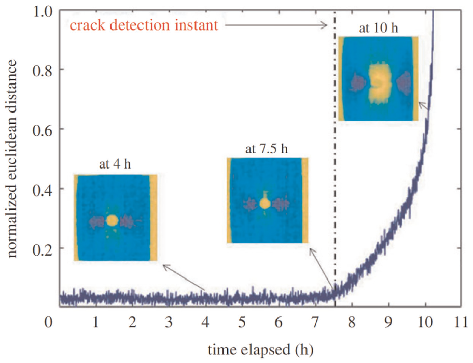
An example of damage monitoring through orthogonal decomposition of CATE data collected during cyclic loading under laboratory conditions. From Amjad et al. ²⁴

System installation

Integrated system

The integrated system consists of sensor units connected to a control computer and a network attached storage server (NAS) through an Ethernet switch. Power is supplied to the sensor units by PoE (Power over Ethernet), via the same Ethernet connections used for communication and data transfer. A bespoke graphical user interface (GUI) has been designed which the operator uses to control data collection, and to access and visualise live and historical data.

Each sensor unit is manufactured from COTS (commercial-off-the-shelf) components, and consists of a Raspberry Pi module, containing the control computer and related control boards, and a sensor module, comprising an infrared sensor (Lepton 3; Lepton 1.5 in earlier systems, FLIR) and a visible sensor (Sony IMX219 8-Megapixel Sensor) with accompanying LED ring light (Figure 2). The Pi and sensor modules can be mounted together as a fixed unit, or, for spatially restricted installations, the sensor module can be fitted at the region of interest with the Pi module at a more convenient location, constrained by the cabling between the modules. Here, a maximum of two units were used concurrently, however a higher number of units can be used simultaneously, controlled by the capacity of the Ethernet switch.

Figure 2.

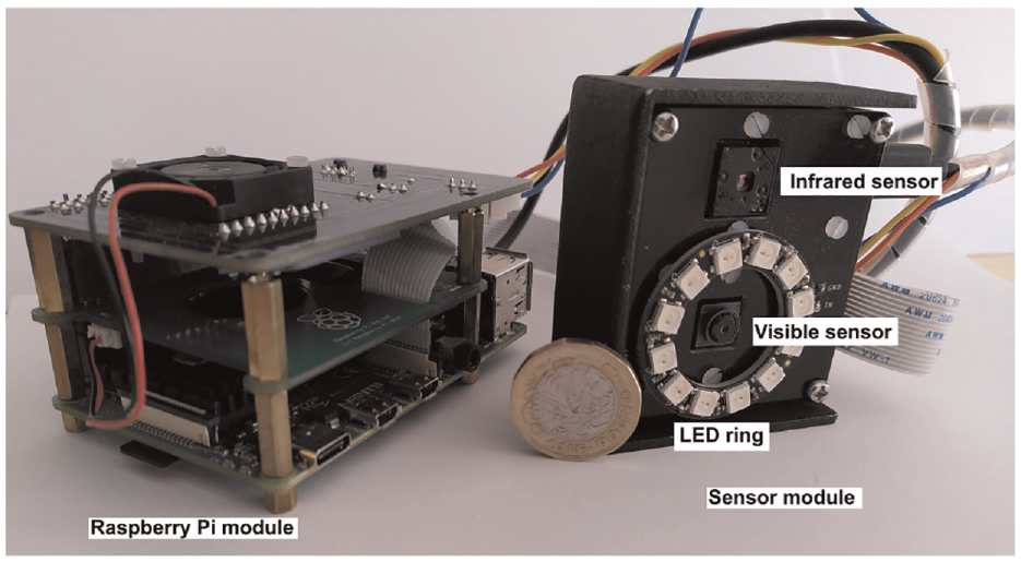
Sensor unit comprising a Raspberry Pi module (left) and sensor module (right) with £1 coin shown for scale.

Once the system is activated through the GUI, all data collection and processing occurs on the Raspberry Pi. Processed data are automatically transferred to the NAS, from which historical and live data can be accessed through the GUI.

As the default setting, resistance strain gauge data is collected continuously at 150 Hz. IR images are collected at 8.8 Hz, and 384 images are integrated to generate a CATE map. ²⁴ Once the infrared images are collected, the LED lights illuminate to allow one visible image to be collected and then processed to generate an uncalibrated DIC strain map. In this way, the LED lights are turned off when IR images are captured, and one DIC image and one CATE map are generated over the same time window.

The CATE and uncalibrated DIC strain maps are then decomposed using orthogonal polynomials,^23,25 and the difference between feature vectors of the reference maps (from the beginning of the test) and subsequent images is calculated and displayed to give a measure of the change in the maps. All codes are implemented in Python, and data processing is carried out on the Raspberry Pi in near real-time (on the order of minutes). The integration of different sensors in one module allows different techniques to be implemented with one system. This allows the system to collect useful data at a range of loading conditions, for which data collection and processing must be adapted to the particular situation.

Two full-scale industrial aerospace case-studies were identified for installation of the sensor system, a fatigue test on a wing and a cyclic pressure test on a fuselage section.

Wing fatigue test

The first industrial proof-of-concept for system deployment using an early version of the system, with Lepton 1.5 sensors was on a full-scale wing fatigue test at the Airbus AIRTeC (Aerospace Integrated Research and Test Centre) facility in Filton, Bristol UK. Two rib-bays were identified for internal installation of the sensor units before closure of the Fuel Tank Access Covers (FTACs). Modules were clamped to stringers on the topside of the wing with sensors facing down to regions of interest on the junction between the front spar and the lower cover (Figure 3). Each sensor unit received input from a dedicated RSG close to its position but out of its field of view.

Figure 3.

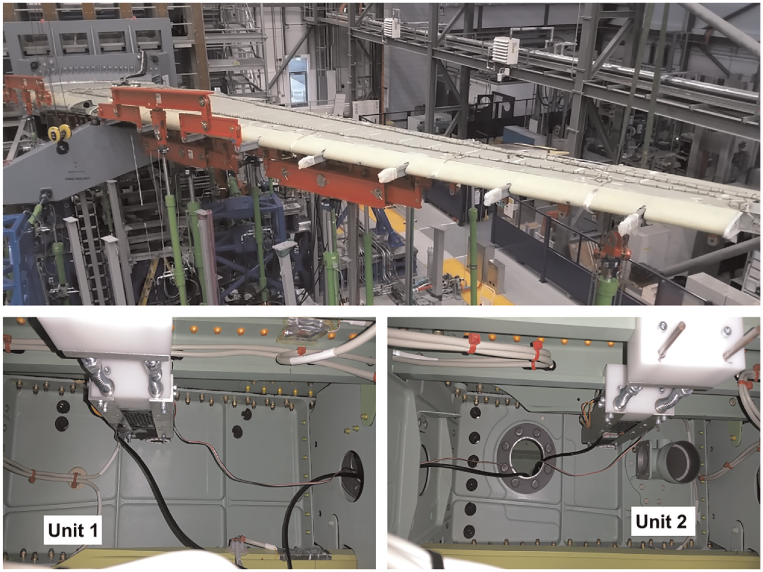
Installation of system in wing fatigue test. Top: View of the fatigue test rig, bottom: two sensor units installed in adjacent rib bays.

The wing was subject to loading representative of loads experienced during flight, and data were collected over several weeks, with output from strain gauges at nominally 150 Hz, visible images at approximately 1-minute intervals, and IR images at nominally 8.8 Hz, with integration of 384 IR images to produce CATE maps at 1-minute intervals. Due to timing and access restrictions to the wing boxes, a speckle pattern was not applied to the regions of interest, therefore visible images could not be processed to generate DIC data.

Fuselage pressurisation test

The second industrial case study was a fuselage section undergoing pressurisation and depressurisation cycles at Airbus, Toulouse, France. Due to travel restrictions during the Covid-19 pandemic, a remote installation procedure was developed in order to guide Airbus personnel through deployment of the system. A crack in the internal frame was identified, and the sensor unit was located to image this region of interest with a speckle pattern applied before data collection began. Figure 4 shows the installation of the system in the internal structure of the fuselage.

Figure 4.

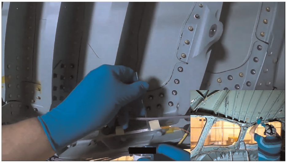
Installation of sensors in a fuselage test. Main image is a view from operator headset, inset figure shows a wide view of the installation area.

Collection of traditional TSA data would require adiabatic conditions which rely on cyclic loading at a high enough frequency.^6,7 The pressure cycle imposed on the cockpit test (on the order of minutes) was considerably slower than frequencies at which traditional TSA is possible. ⁶ The CATE approach is less reliant on the identification of stress hotspots, as the shape of the entire FOV is interrogated due to the use of orthogonal decomposition, and has been shown to give a quantitative measure of damage growth at relatively low loading frequencies, for example, 1 Hz for coupon specimens undergoing cyclic fatigue loading. ⁹ Therefore, before system installation on the case study, laboratory testing on coupon specimens was carried out at equivalent frequencies to those at the industrial site to determine if CATE data could be collected. It was determined that even with the shape analysis approach, no viable data could be collected with the CATE thermal method, therefore only RSG and DIC data were collected from the fuselage section.

For this application, an algorithm was implemented to collect visible images at the peak strain measured by the RSG during pressurisation cycles in order to show the largest uncalibrated strain concentrations in the DIC images, and allow for simpler comparison between DIC maps. A reference image was collected by the operator at the beginning of the test, and subsequent images were processed using the DIC code to generate uncalibrated maps of maximum principal strain. Processing of uncalibrated DIC strain maps and the calculation of the feature vector differences were carried out on-board the Raspberry Pi module, then transferred to the NAS.

Results

Restricted access wing installation

The system was successfully deployed within two rib bays in the wing and strain gauge data and visible and infrared images were collected during the fatigue loading. The infrared images were combined with the local strain data reported by the gauge to generate CATE data. An installed sensor unit and example outputs are shown in Figure 5. Data was successfully collected from inside the two wing boxes during representative fatigue loading over several weeks.

Figure 5.

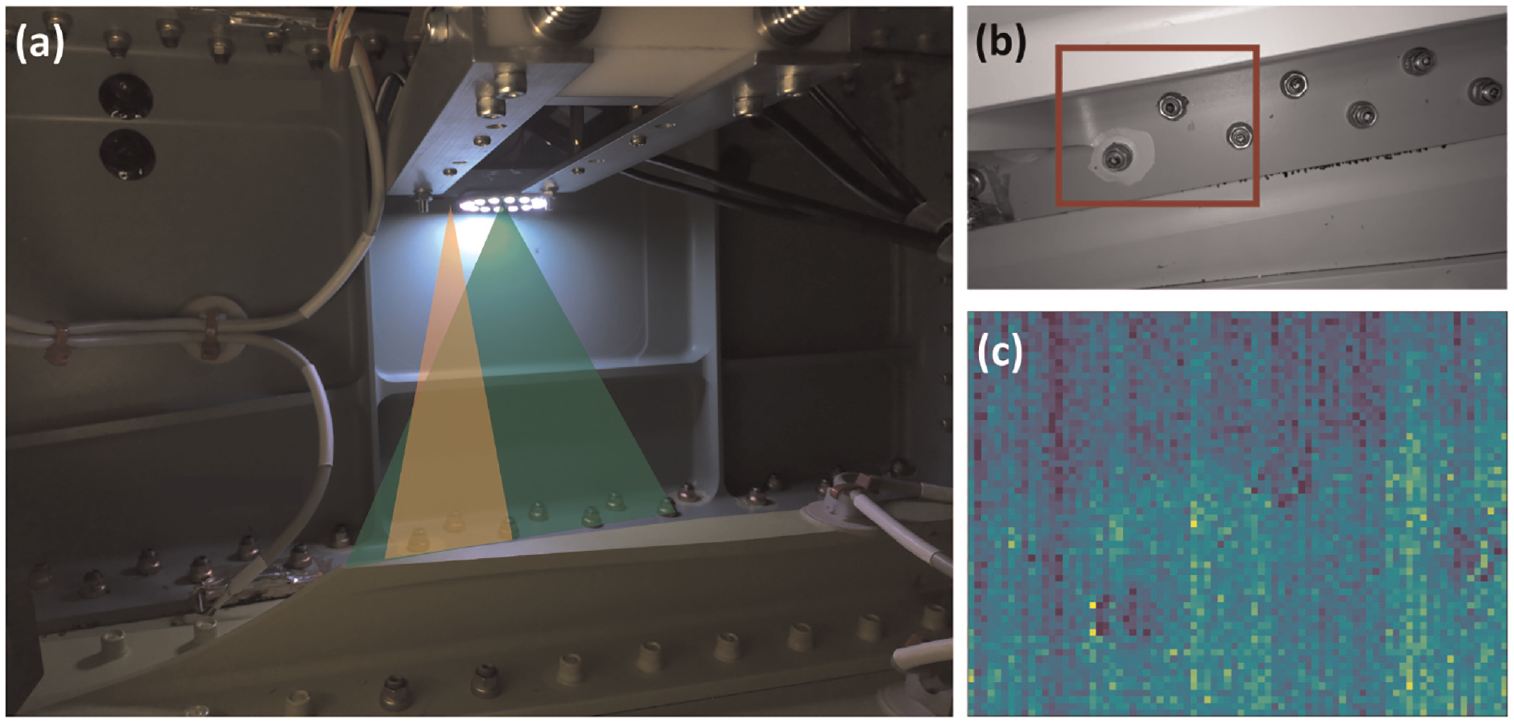
(a) sensor module installed in rib bay, overlain triangles illustrate approximate Fields of View (FOV) for infrared (left) and visible (right) sensors; example outputs from (b) visible sensor and (c) CATE data map. The red rectangle in (b) indicates the approximate FOV of the CATE map.

Although time and access restrictions did not allow for speckle application, the consistent output of visible images suggests that DIC processing would be possible using data from this, or a similar, installation. The CATE map in Figure 5(c) shows the position of rivets, likely due to the relative motion of the camera compared to the field of view, but there are no other indications of stress concentrations. No damage was expected to develop in the rib-bays monitored during the timeframe of data collection on the wing. Therefore, the absence of observed stress concentrations or changes in CATE maps was an expected result.

Damage detection in fuselage test

Data were collected from the fuselage test over a period of months, with some intervals where loading was paused, for inspection or repair. One repair was carried out on the crack in the internal frame that was inside the FOV of the system. Figure 6 shows the uncalibrated strain maps indicating the crack position pre- and post-repair. As the orthogonal decomposition technique relies on comparisons between datasets, it is not necessary for strains to be calibrated, and therefore only relative values are shown in these uncalibrated strain maps. Due to differences in pressurisation before and after repair, it was not possible to collect images at the same local strain as reported by the RSG. However, the effect of the repair can be observed, as similar local values of uncalibrated DIC strain are reported, even at higher pressurisation.

Figure 6.

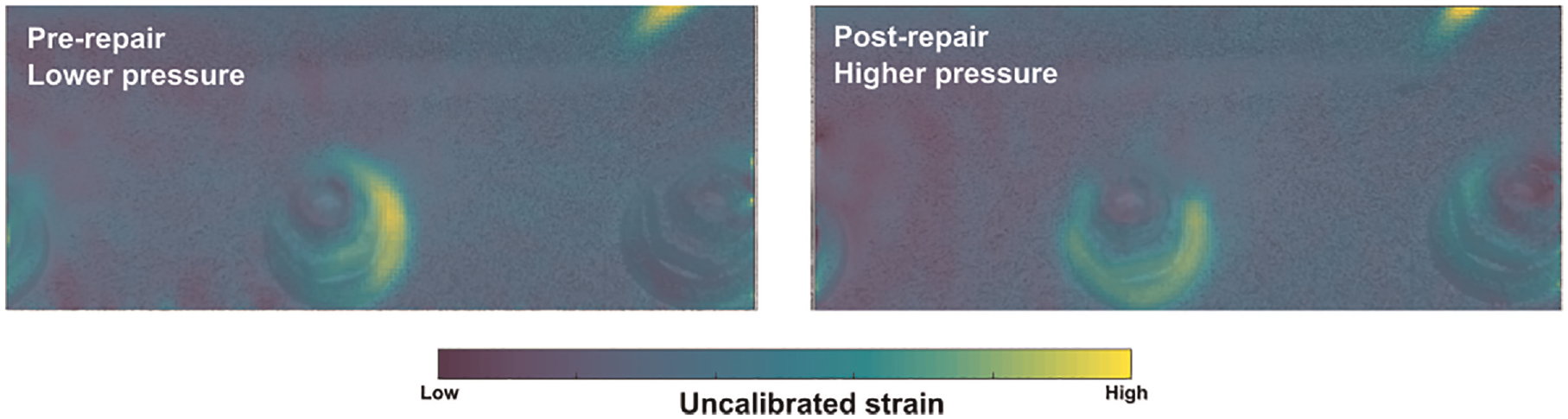
Uncalibrated maximum principal strains pre- (left) and post-repair (right). The fuselage was pressurised to a higher level after repair (by a factor of ~2), but the local strains related to the crack are similar in both.

Uncalibrated DIC strain maps were decomposed, and the feature vector difference reported between a reference image and later images. Unfortunately, after the repair shown in Figure 6, the sensor module was accidentally repositioned during a routine inspection. This resulted in a new FOV, so a new reference image was collected for the calculation of the feature vector difference.

The repositioning of the sensor unit also resulted in an irregular connection between the sensor unit and the processing computer, which interrupted the data collection algorithm. To solve this problem on a time scale that allowed data collection during the test, the algorithm was modified so that a series of visible images were collected and processed at, or near, peak strain. To exclude images collected during depressurisation and when the peak strain was no longer being experienced, the timing between images was interrogated in post-processing and only results from one image of each of these series were reported. For simplicity, the first image of each series was chosen. The feature vector difference after repositioning until the end of data collection is shown in Figure 7, along with example uncalibrated DIC strain maps at given times.

Figure 7.

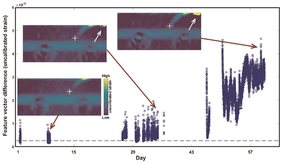
Feature vector difference against time for the FOV during the pressurisation test. Data points related to images collected during depressurisation have been excluded during post-processing (see text). Inset figures show uncalibrated maximum principal strain maps from DIC processing. Overlain white cross is shown at the same position in each inset figure and can be used as a reference for the reader to visualise the evolution of crack position with time. Arrows indicate development of a secondary strain concentration. Horizontal dashed line represents the noise floor, here defined by averaging the standard deviation of a series of uncalibrated strain datasets collected at zero load. ²⁶ Gaps indicate times when the loading was paused.

Crack growth is seen in the inset figures, as the crack tip moves further into the FOV, and a secondary strain hotspot develops. The appearance of this new strain concentration may be related to the growth of a new branch of the crack, close enough to the FOV to influence the strain field. These changes correlate to an increase in the feature vector difference. In contrast to the well-defined curve shown in Figure 1 from laboratory testing for simple loading, this line shows a significant amount of variation.

This variation in the feature vector difference may be due to slight differences in the maximum pressure experienced during each loading cycle, or visible images not being collected at the exact peak pressure for each cycle. Despite the noise, an increasing trend can be observed, particularly in data collected after day 29. Further processing of this signal could reduce the noise, but care would have to be taken to avoid removing details representing real changes if a smoothing approach were used. Alternative approaches could involve improvements in the triggering of image collection or normalisation by the applied load where known.

A band of, what appears to be, higher strain concentration above the rivets has appeared when comparing these inset figures to the pre- and post-repair data. This may be related to the problems of repositioning, and resultant images being slightly out-of-focus in this area.

Discussion

The results of the industrial installation tests show that the prototype system can be mounted stably in spatially restricted industrial environments, undergoing significant loading representative of that experienced during flight. As the system has a low volume and mass it can be positioned in a way in which it does not disrupt necessary functions of the structure or test, and allows required access for visual inspection. This, combined with the integral lighting system, expands monitoring capabilities from previous external mounting options, to allow observation and tracking from within the structure. As shown in the fuselage test, this system is capable of detecting and monitoring damage.

Despite the lower sensitivities and resolutions of the integrated sensors when compared to more expensive traditional systems, the use of orthogonal decomposition to process the collected images results in a quantitative representation of the change in full-field data. As this is reported in near real-time, this information can actively inform decision-making, for example in test protection or in-service use. As data is collected continuously during condition monitoring, this represents opportunities on different timescales – in the short-term, near real-time alerts can indicate to an operator that something has changed. Historical comparisons are also possible, for example trends in raw data from a point sensor can be used to detect a change in structure compliance.

When a sufficient number of terms is used in data decomposition, the feature vectors can be used to reconstruct the data. For long tests that produce a large amount of data, this decomposition approach would allow the full-field data to be processed and then deleted, to save only the feature vectors, which are orders of magnitude smaller than the original data. However, the number of terms would need to be carefully considered before data collection, and it should be noted that fewer terms are needed for decomposition to detect damage than would likely be required for high resolution data reconstruction.

As reported previously when applying orthogonal decomposition to damage detection, the quantitative value output from this approach does not immediately indicate crack length or location, but indicates the extent of damage in the full field of view analysed. ⁹ Some interpretation or further analysis would therefore be required to output crack measurement values. As this orthogonal decomposition technique has been shown to indicate crack growth on the order of a millimetre, ⁹ which is significantly shorter than current visual inspection methods, one possible application would be to use this technique as an early warning system to indicate to an operator where further inspection and measurement is required.

The use of the system in the two case studies has also highlighted other areas of limitations, or challenges for industrial use. For example, in the fuselage test, tracking changes due to damage using the feature vector difference was disrupted due to accidental relocation of the sensor module. As module removal and repositioning is a likely occurrence during inspections, a more robust approach is required to allow reliable results, for example by regular updating of the reference image in a Lagrangian approach.

The variability of the feature vector difference seen in the fuselage test is likely caused by image collection at different pressures. If this feature vector difference data were to be used in industrial environments, for example to make decisions regarding test interruption or to trigger a traditional inspection, the uncertainties introduced by the variability in Figure 7 would need to be considered and reduced, to ensure reliability. In the fuselage test, the algorithm located a high point in the load cycle, but this was not at a consistent level throughout the test, due to differences in the pressurisation. Therefore, one approach to reducing this variability and decreasing uncertainty would be to introduce a more effective ‘trigger’ for data collection.

Despite these limitations, the proof-of-concept case studies show that this system has great potential for use in structural health monitoring, not only in aerospace applications but across many industry sectors. The ability to apply the orthogonal decomposition approach to uncalibrated full-field strains or stresses introduces an advantage in industrial environments where calibration may be impossible. Due to the size and cost of these sensors, it is also conceivable that a network of such sensors could be installed as an array, covering a larger area or focussing on several regions of interest. An array of sensors would also allow more advanced processing, for example data from multiple point sensors could be analysed to triangulate the location of damage initiation in a structure.

The low cost of these sensors, and the units as a whole, would also allow this system to be installed in extreme operating conditions, where traditional systems would not be installed due to the risk of damage. The integration of several sensors within one module also allows different NDE techniques to be applied at different times or as loading conditions change. The decrease in size and cost of the system when compared to current sensors available on the market shows that these sensors also have the potential to be installed for in-service condition monitoring.

Conclusions

A prototype structural monitoring system has been developed which uses COTS components to combine multiple NDE measurement techniques in one unit. The combination of strain gauge input, and measurement techniques based on TSA and DIC allows data to be collected under a range of loading conditions. Data are collected and processed in near real-time, with the application of orthogonal decomposition resulting in a quantitative representation of the surface changes due to damage growth.

The system has been applied to two different industrial case studies demonstrating that it can be installed and used in spatially restricted, internal aerospace environments. The system can acquire, process and deliver appropriate data on a useful timescale to support critical decisions about fatigue tests on structural systems. This system represents a step towards in-service monitoring where damage development and growth can be indicated in near real-time.