The traditional solution for the stresses below an elliptical Hertzian contact expresses the results in terms of incomplete Legendre elliptic integrals, so are necessarily based on the length of the semi-major axis a and the axis ratio k. The result is to produce completely different equations for the stresses in the x and y directions; and although these equations are now well-known, their derivation from the fundamental, symmetric, integrals is far from simple. When instead Carlson elliptic integrals are used, they immediately match the fundamental integrals, allowing the equations for the stresses to treat the two semi-axes equally, and so providing a single equation where two were needed before. The numerical evaluation of the Carlson integrals is simple and rapid, so the result is that more convenient answers are obtained more conveniently. A bonus is that the temptation to record the depth of the critical stresses as a fraction of the length of the semi-major axis is removed. Thomas and Hoersch’s method of finding all the stresses along the axis of symmetry has been extended to determine the full set of stresses in a principal plane. The stress patterns are displayed, and a comparison between the answers for the planes of the major and minor semiaxes is made. The results are unchanged from those found from equations given by Sackfield and Hills, but not previously evaluated. The present equations are simpler, not only in the simpler elliptic integrals, but also for the “tail” of elementary functions.
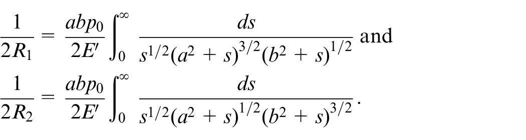
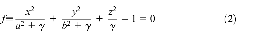
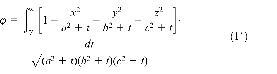
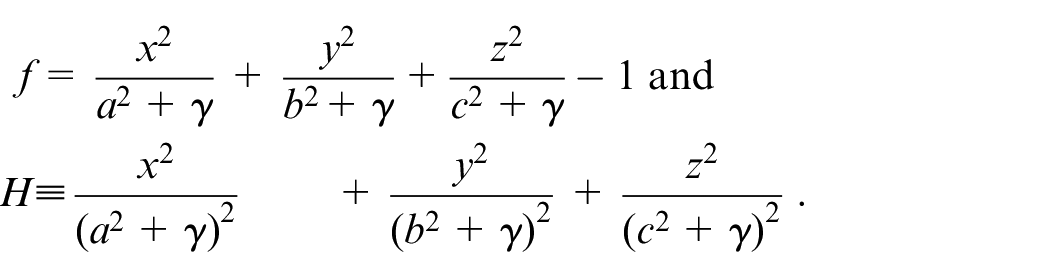
The analysis of elliptical Hertzian contacts is most conveniently done using Love’s potential function1, where is the positive root of
Thus, from Johnson’s Contact Mechanics,2 the displacements due to a Hertzian pressure distribution are ,
Within the loaded region we require , so that (since within the loaded region ), we have
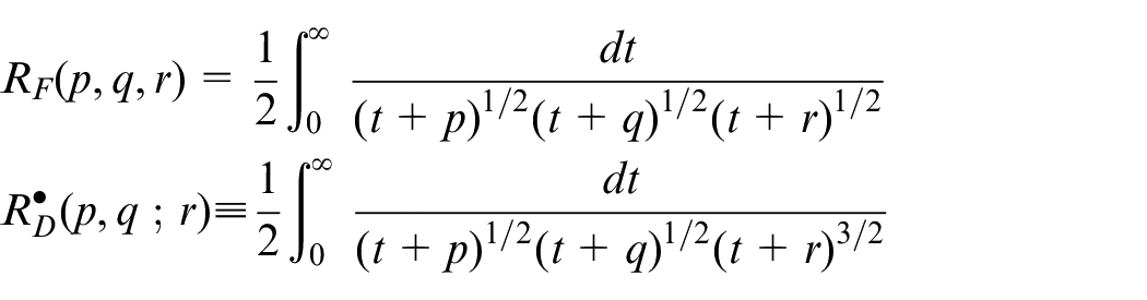
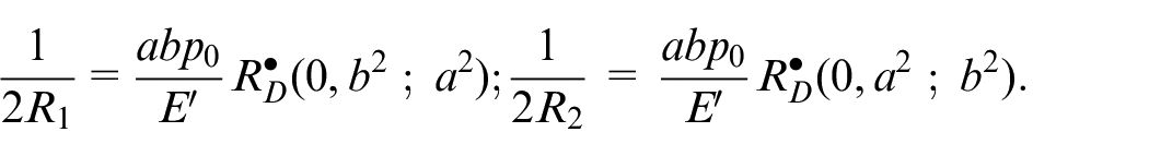
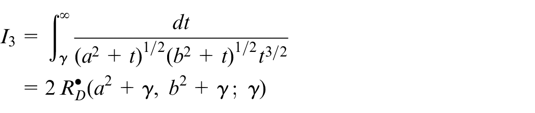
Those with considerable mathematical dexterity can transform these integrals into Legendre elliptic integrals ( and (where )); but an easier alternative is to use Carlson elliptic integrals, defined as
(Carlson3 or Greenwood4 (Note that all three parameters in are interchangeable, but only the first two in . indicates that this is one-third of Carlson’s )). Now no mathematical dexterity is required to see that
(Equally readily, the displacement is found to be .)
Thus, using the natural affinity between Love’s potential function and Carlson elliptic integrals, we have replaced a pair of strongly differing equations by a pair of simple equations. Actually, we have done better than that: we have replaced the pair by asingleequation. For the curvature in the x-direction, the square of the semi-axis in the x-direction is the third argument: for the curvature in the y-direction, the third argument is the square of the semi-axis in the y-direction. We have a single equation, readily obtained, with no mention of major and minor axes.
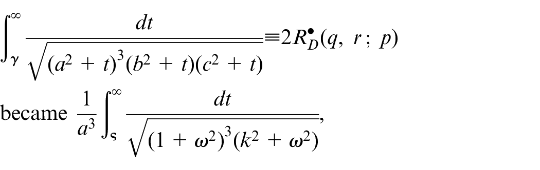
True, there are no tables of Carlson integrals, and it appears that the two functions K(e) and E(e) of a single variable have been replaced by two functions of two variables. But here the Carlson scaling laws come in. A simple change of integration variable (substitute ) shows that and , so that one argument can readily be reduced to 1. Thus the complete Legendre integrals of a single variable can be replaced by Carlson integrals with two passive arguments (0, 1) and calculated as functions of the single remaining variable. The incomplete Legendre integrals, functions of (more often denoted by or ) and the modular angle could be replaced by Carlson integrals with just two active arguments (i.e. differing from unity). In the computer age, this will probably never be done: a very simple, very rapid algorithm for calculating Carlson integrals is available. It is as simple as the recommended algorithm for the complete Legendre integrals, and since the same algorithm is used for all arguments, is distinctly preferable to the usual method for incomplete Legendre integrals.
A previous article4 shows the advantages to be gained by the use of Carlson integrals in the analysis of the surface properties of Hertzian contacts: the determination of the contact geometry as cited above, the determination of the surface stresses under normal pressures as discussed by Hertz, and those caused by tangential loads as studied by Mindlin and others. Here we consider to what extent the analysis of the subsurface stresses could equally benefit.
The prospective advantages are of course the same: (1) Natural affinity between Love’s potentials and Carlson integrals (2) No need to distinguish between major and minor semi-axes: to assume and focus on the ratio : (3) Treating the two directions equally promotes a beneficent mind set: (4) The convenience of ending with a single equation instead of two, usually very different, ones. And to the author, perhaps alone, the advantage of dimensioned equations, providing an immediate check for errors: others may not need this!
The convenience of Carlson integrals over complete Legendre integrals is perhaps minor, the real gain is in the easier derivation: but see Discussion for what happens when we encounter incomplete Legendre integrals.
Analysis of Elliptical Hertzian Contact
The basis of the solution is spelt out by Love,1 and taken on from there by Thomas and Hoersch,5 [“T&H”] and it is hard to improve on their presentation, up to the point where they are reduced to converting their answers into Legendre integrals, and so forcing their admirable, symmetric, equations into the inevitable contorted form.
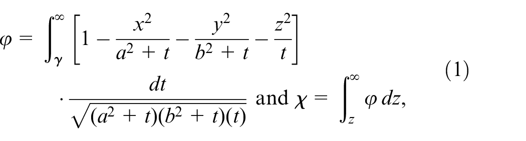
Love introduced two potential functions ϕ and χ, defined as
where is the largest root of
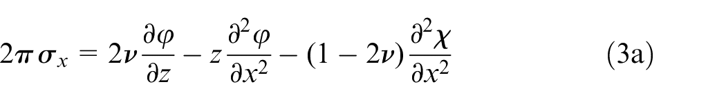
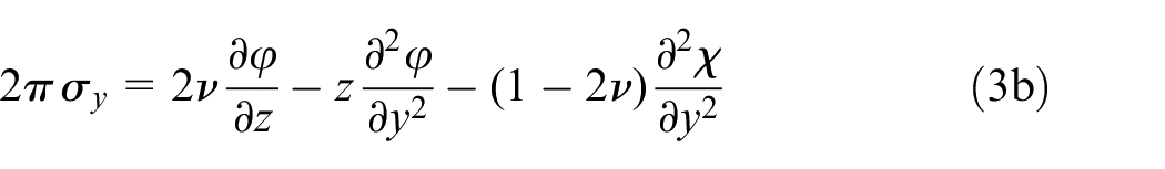
Love gives equations only for the displacements: it seems that T&H were the first to continue and find the strains and hence obtain the basic equations for the stresses (see also Johnson2 or Hills et al.6 (HNS)).
(A factor will subsequently be inserted for a Hertzian pressure distribution.)
The equation for , which we do not need, is given by Johnson2 and Hills et al.6 added
Note the complete symmetry between the pairs and : this is lost in the final answers when Legendre integrals are used, but is preserved when we use Carlson integrals.
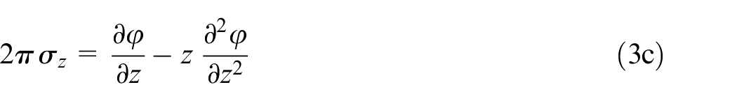
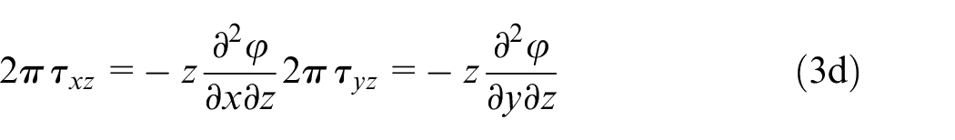
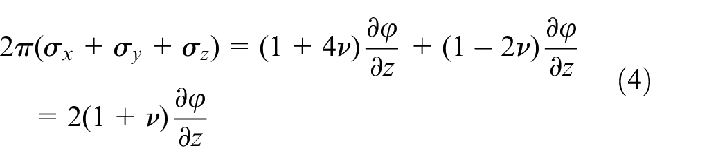
Since ϕ and χ are both harmonic, and so that , then from equations (3)
We note that is independent of the second potential function . Indeed, not all the stresses involve χ, or elliptic integrals; for are all elementary functions, independent of ν.
Extracts from Thomas and Hoersch’s analysis
We introduce a spurious , which is identically zero, in order to make clearer the permutations to obtain from : thus we write the potential (1) as
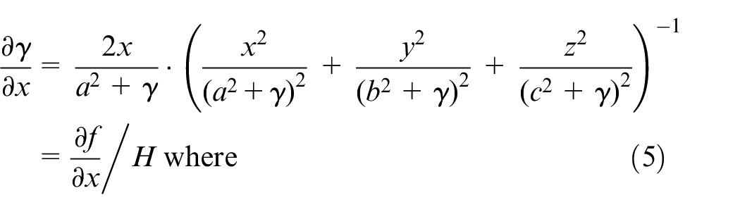
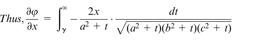
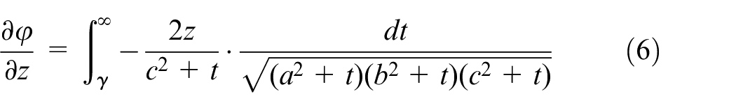
Differentiating is straightforward, but lengthy. The derivatives of both integrand and lower limit are needed, (though not for the first derivative, for there the integrand vanishes) and T&H show that
and permuting,
This is readily seen to be .
Hence, for our Hertzian contact,
The second derivatives involve both terms: thus
which, by writing ; ; , becomes
Using Carlson integrals this is
Permuting the symbols gives
Note that .
For the derivative of the integrand vanishes, leaving (using (5)) just
From the basic equation (3) it will be clear that for an incompressible solid these are all we need: reduces to , while for all values of , (and equally from (3d) we can obtain ).
Otherwise we need the second potential χ. T&H begin by showing
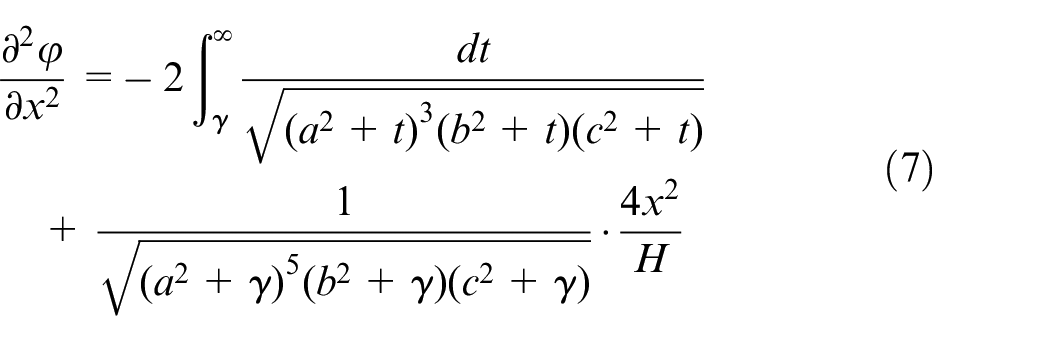
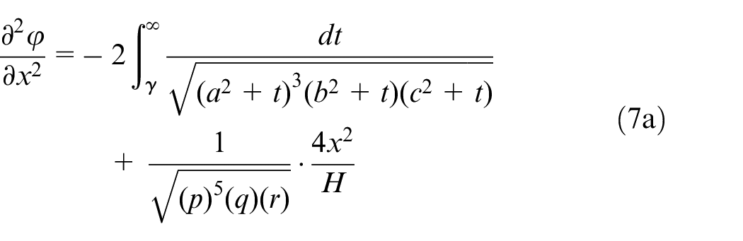
and we need to differentiate (7a): .
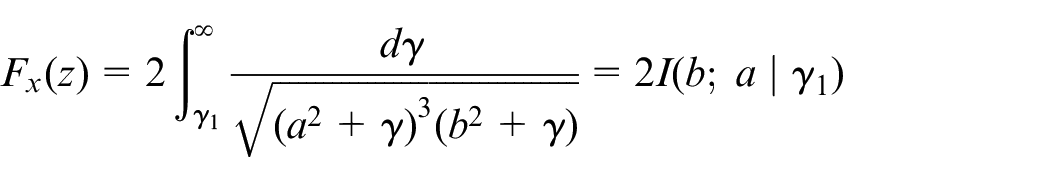
The differentiation is practicable only when the second term is absent: so for (only) we have
where the in the numerator is itself and makes the integration difficult! But on the axis we have simply : so substituting (and dropping ) we get:
and T & H show that the integral equals as is readily checked by differentiation. T&H stop there, with an equation that appears to fail for a circular contact, but a little algebra gives
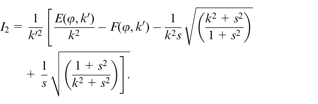
However T&H needed numerical answers for their stresses, and in 1930 the only elliptic integrals available were Legendre’s: so they transformed (spoilt?) their beautiful, symmetric, integrals by substituting and writing , so that, for example, the integral (7a)
which they identified as (where and . (Inconsiderate of Love to use for his potential the standard symbol for the modular angle)).
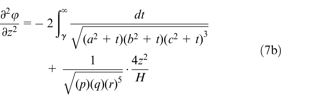
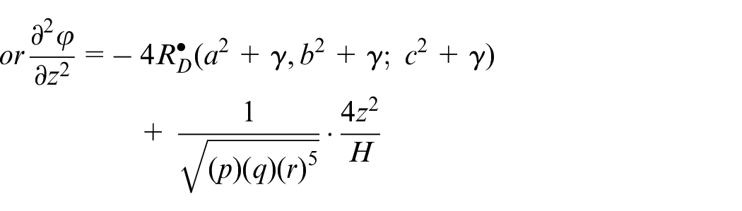
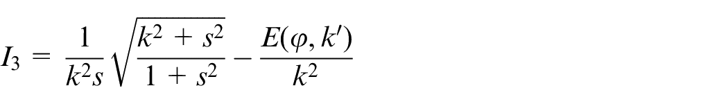
But the integral (7b), which we know from symmetry to be ,
was found to become +algebraic terms (see Discussion).
The Carlson forms needed no changes of variable or careful mathematics, and retain the natural symmetry.
Stresses on the axis of symmetry
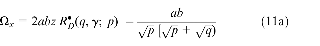
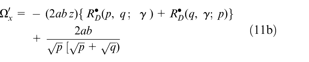
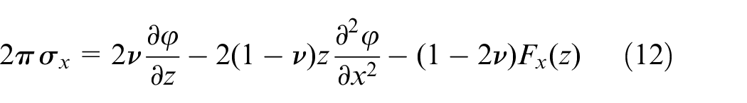
The stresses are conventionally given as the sum of the answer for and a term proportional to , as , so we have (after restoring the factor )
Using Carlson integrals, and ,
(on the axis the algebraic term disappears). and also, from (9), (10), .
Then since on the axis , the stresses are
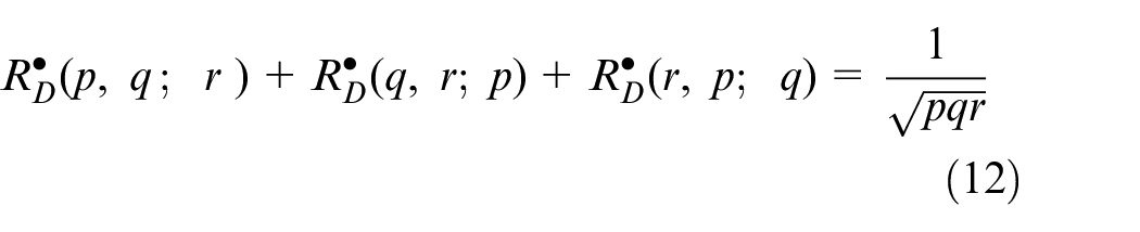
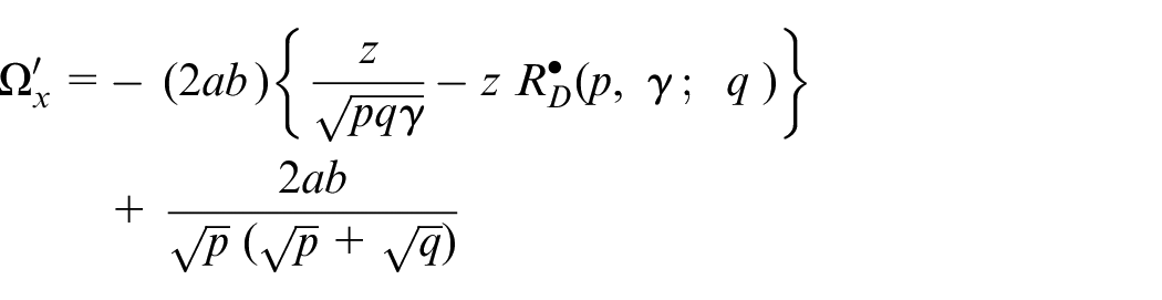
There is a problem here, for at , is infinite (though the product is finite): but we evade this by using the identity
(proved in Greenwood4 (Appendix A3); quoted (in a different notation) in Hills et al.6 (10.52)).
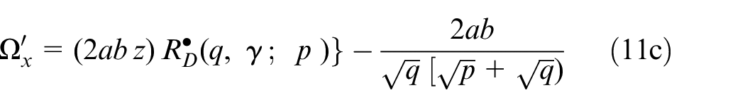
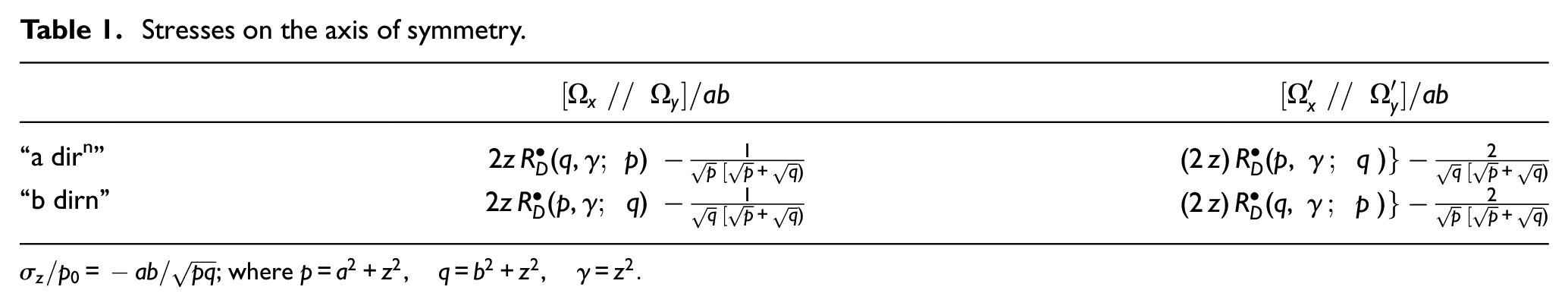
To bring out that a simple permutation is all that is needed to give the stress in the b-direction, the two results (11a and 11c) are displayed as Table 1 (We have used the permuted ).
Stresses on the axis of symmetry.
“a dirn”
“b dirn”
; where
It must be emphasised that these are not the two distinct equations for the stresses along the directions of the major and minor axes: they are the stresses along the “a” and “b” directions, either of which might be the major semi-axis of the ellipse: there is really only a single equation.
Verification
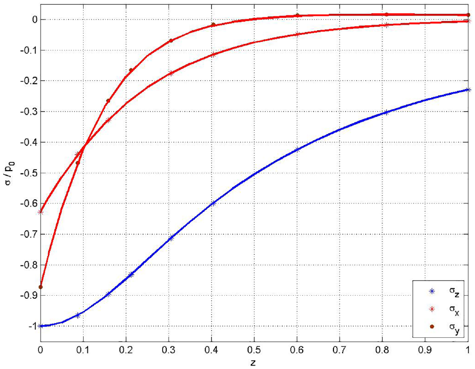
Thomas and Hoersch,2 with the handicap (in 1930) of working from tables of incomplete Legendre functions at intervals, tabulate the stresses on the axis for and a number mildly elliptical geometries (appropriate for wheel on rail contacts). Their answers are related to the principal curvatures at the contact, but have been converted to values of by taking the value they give for at to be . For their moderate case, there is almost perfect agreement with the present calculations (occasional in the fourth decimal). Figure 1 shows the (less good) comparison for , the markers being the T&H scaled values: the lines the present ones. It is clear that the present equations using Carlson integrals are completely equivalent to the T&H equations using Legendre integrals.
Comparison of present answers with results tabulated by Thomas and Hoersch.
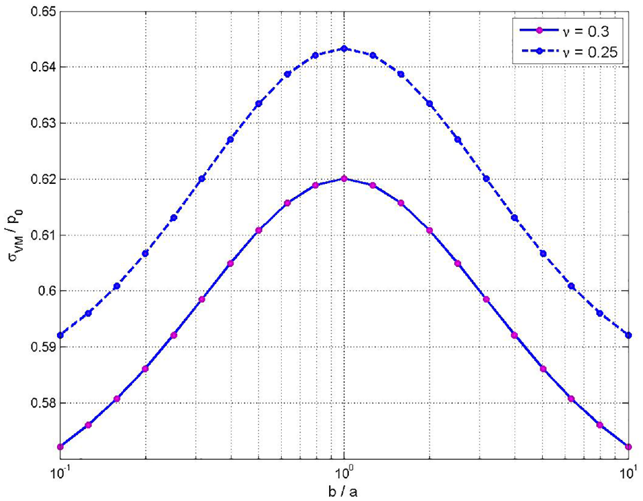
It is well-known that for a circular contact the value of the critical stress on the axis depends on Poisson’s ratio, and T&H’s equations have always allowed an investigation of how this result transfers to elliptical contacts, but seems not to have been done. It is very readily accomplished using the equations above, and Figure 2 shows the result.
Maximum von Mises stress. Poisson’s ratio has a significant effect.
Note that we plot the values of the greatest von Mises stress on the axis, defined as . The maximum is for a circular contact, and for is . Johnson6 quotes a critical stress of , but this is for the maximum principal shear stress, here equal to . For a circular contact where this is indeed just half our von Mises stress.
Progress so far
A single, simple equation has been derived from which both the stresses on the axis and can be found by permuting the variables. These replace the pair of more complicated equations derived by T&H. T&H regard converting their symmetric integrals into Legendre incomplete elliptic integrals as “the authors’ innovation”: and comment “The direct derivation of these results is rather tedious” (it is not given). Perhaps I should write “the present innovation is converting the integrals into Carlson elliptic integrals” and “The direct derivation of these results is quick and straightforward”!
The full stress distribution on a principal plane
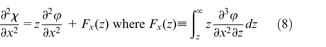
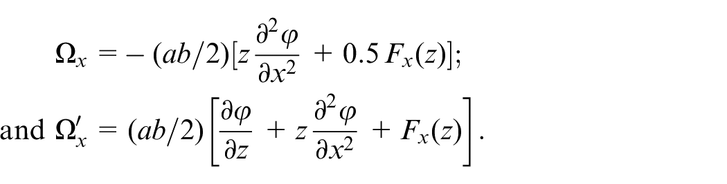
The general equations still hold, so combining (3a) with (8), we get
where providedx = 0.
In describing the evaluation of for points on the axis, the actual significance of has been glossed over. It is a contribution to from points in the y-plane . For points on the x-plane →the plane containing the major axis →we need to use , and this will only give us , not the in-plane stress . However since equation (4) for does not involve , (nor does ) this is good enough: so oddly, to find the in-plane stresses on a principal plane, we find the out-of-plane stress!
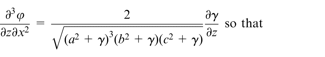
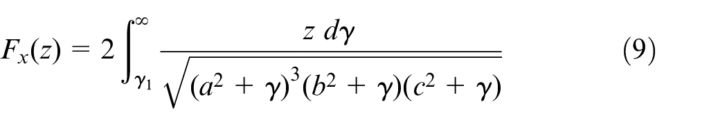
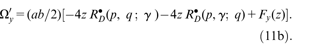
The switch from to simply requires the interchange of and , but the evaluation (of either) will now be harder, for again the integrand contains both explicitly and implicitly as . But the relation is no longer the simple : instead (for the plane) it is . However the reverse relation is usable, and converting the original integration wrt into integration wrt becomes possible. The somewhat involved procedure is described in the Appendix: we note here that the forward relation – finding as the positive root of a quadratic – is still needed, but now only to determine the lower limit of integration: it does not enter the integrand. Recalling equation (9) for but using its dual to benefit from y = 0 on the x-plane and so obtain , we have
From the Appendix, we have
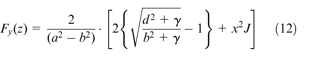
where
where (but see Appendix for d = b, i.e. for )
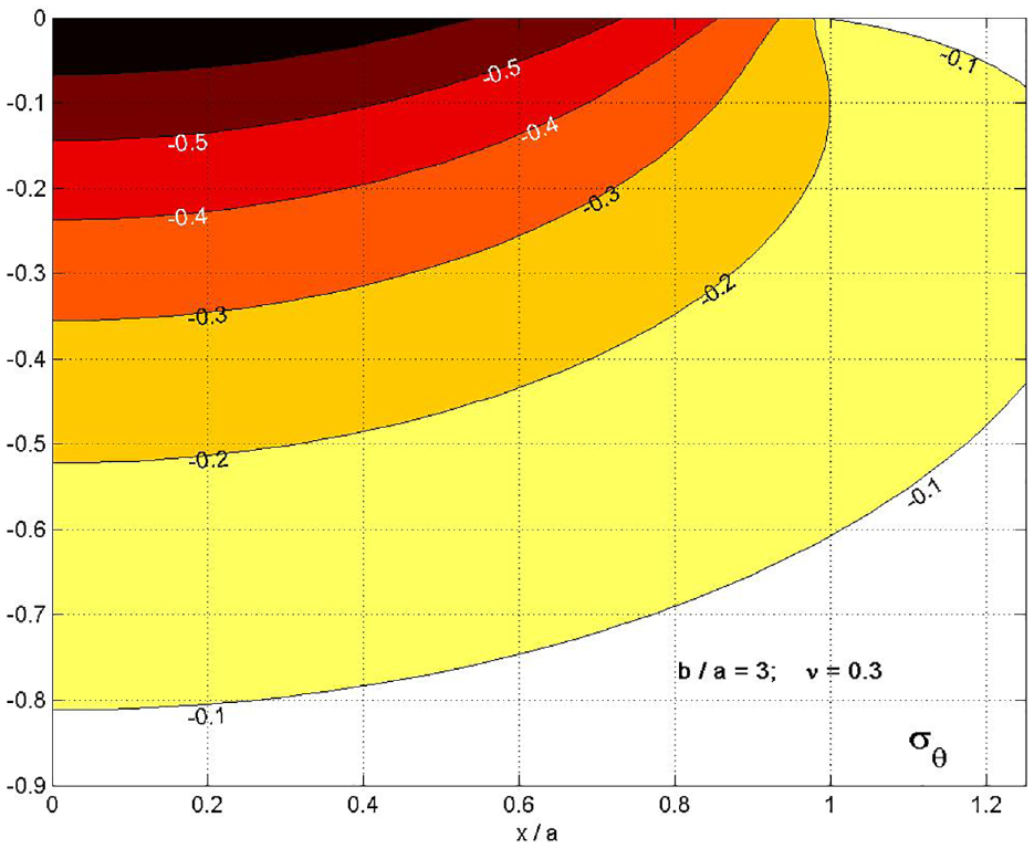
To avoid the confusion of denoting the in-plane principal stress as when on the plane but as for the plane, we shall (as for a circular contact) use for the radial, in-plane, stress and for the out-of-plane stress. Thus, equations (11) are for and give the hoop stress
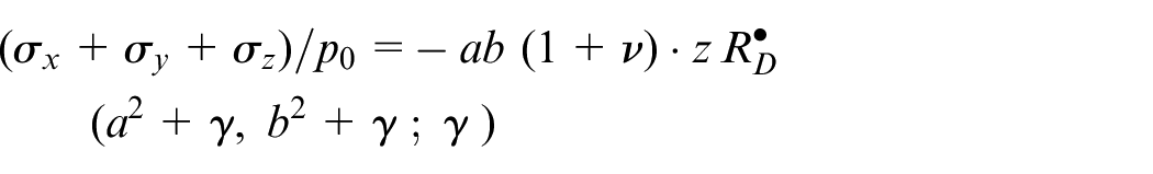
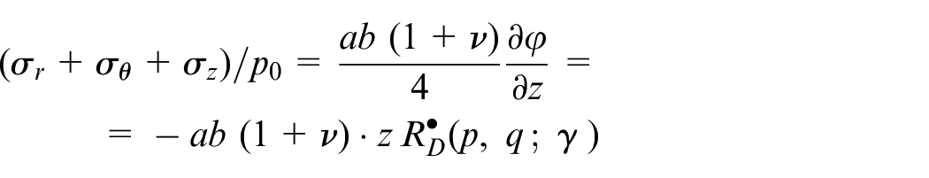
The sum of the principal stresses is given by equation (4), which with the factor included becomes (using (6)):
(Note that on the surface within the contact area, the product must be replaced by its limiting value (the mathematical limit, not just copied from Hertz!)).
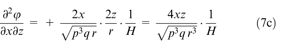
Then, since for the normal stress we have (7c) we at last obtain the radial stress .
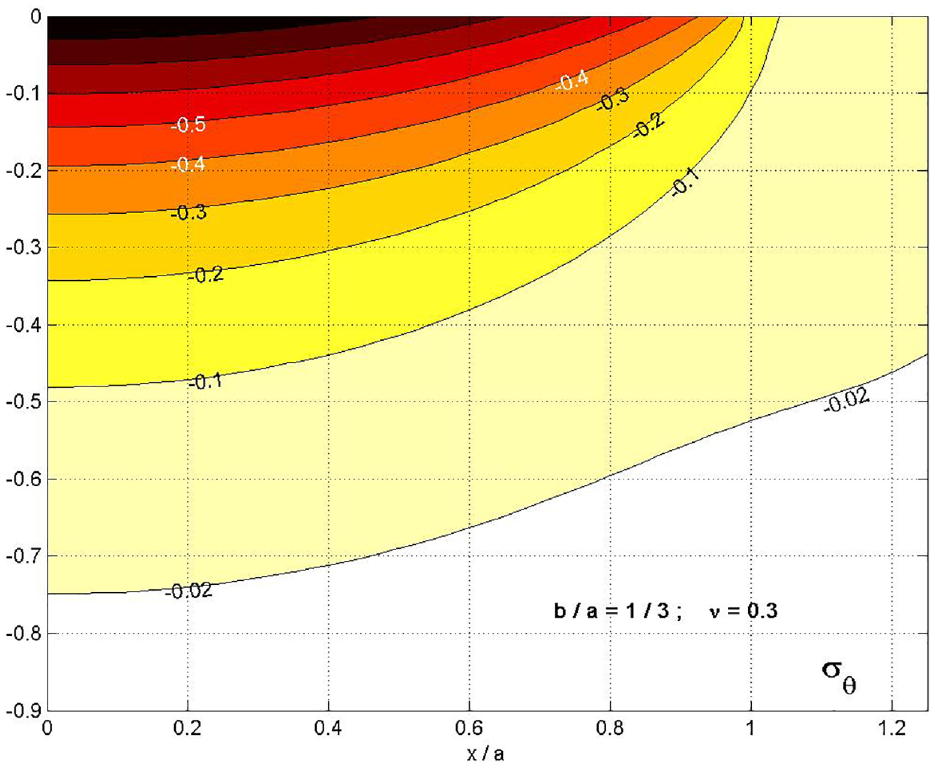
Figure 3 shows a typical hoop stress distribution. It is indeed much the same as for a circular hertz contact. In the region shown, the hoop stress is entirely compressive, and almost entirely confined to the region below the contact area. The greatest values are of course on the axis, and the greatest value is (for ) close to . But as is known for a circular contact, and as found by Thomas and Hoersch (and here: see Figure 1), at greater depths very small (hoop) tensile stresses are found. Note a problem of identification here: on the axis , which is the hoop stress?].
Hoop stress distribution on the principal plane containing the major axis.
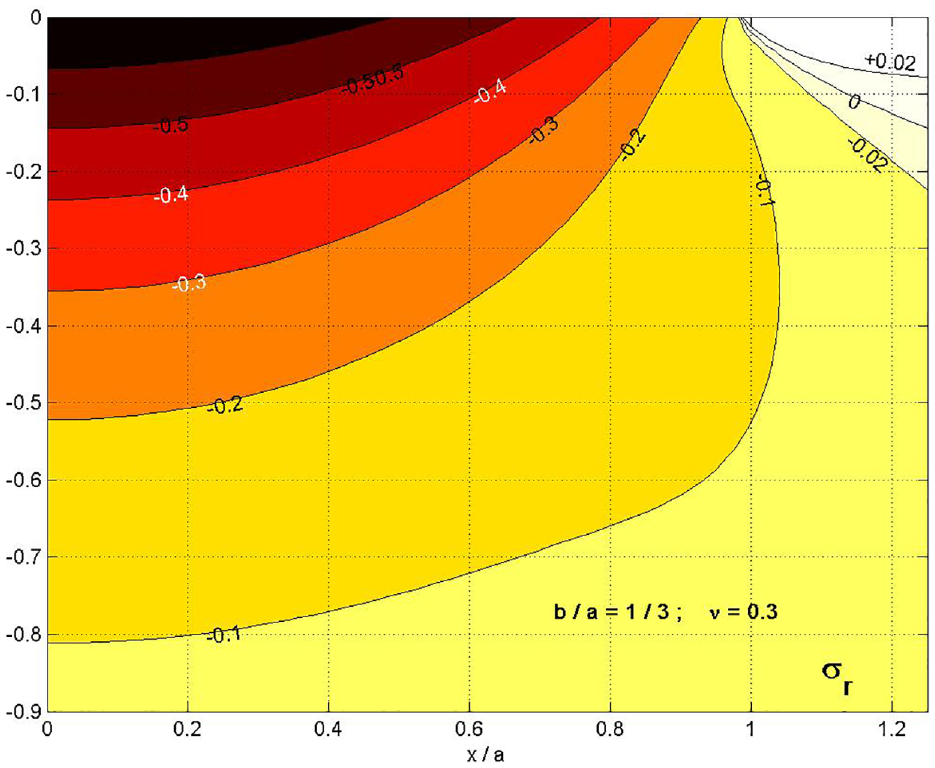
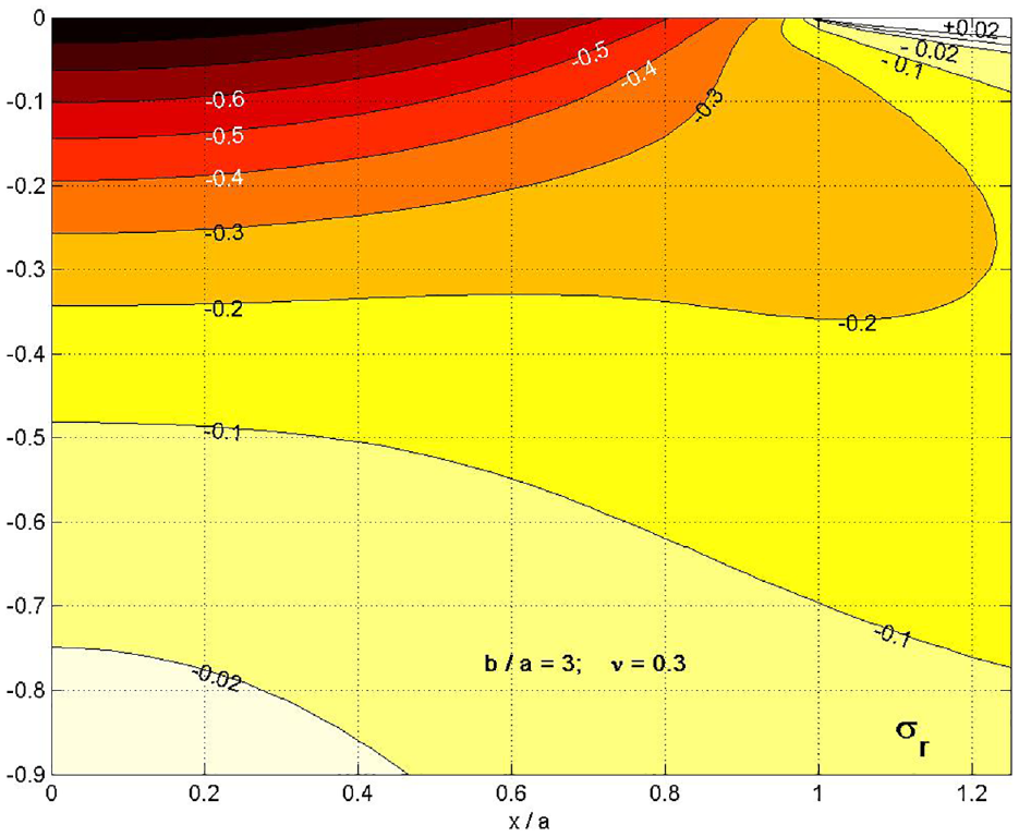
Figure 4 shows the matching radial stress distribution. Some differences from the hoop stress distribution are clear. The radial stresses extend substantially further down than the hoop stresses; but this we have already seen from Figure 1 showing the stresses along the axis (for a similar geometry but ). For , we find that at on the axis, while the hoop stress has fallen to , so this is quite different from a circular contact, where on the axis, the two must be equal.
Radial stresses on the principal plane containing the major axis.
In contrast, Figure 5 shows that the surface stresses do behave as for a circular contact, with the hoop stress not falling to zero at the contact edge, while the radial stress has become tensile there; and as for a circular contact becoming equal and opposite outside the contact. Figure 4 brings out that the tensile region is not purely at the surface, extending to perhaps (though whether this is a sensible measure, here on the a-axis, is not clear for comparison, we need to examine the stresses on the principal plane along the minor axis.
Hoop stresses in the principal plane of the minor axis.
Not surprisingly, significant hoop stresses exist much further beyond the edge of the contact area, although Figure 7 shows that actually on the surface, the behaviour is the same as for a circular contact. The radial stresses (Figure 6), somewhat to my surprise, show the same tendency more strongly.
Radial stresses in the plane of the minor axis.
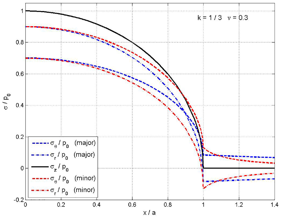
Surface stresses along major and minor axes for .
Figure 7 compares the surface stresses along the major and minor axes. We see that they are what one might expect from a knowledge of the pattern for a circular contact. Here they decay from the values at the origin to the known values at the ends of the axis2 (CM 3.68a), followed by a state of pure shear (). The surface stresses outside the contact area decay, but the variation as for a circular contact is found only when or is large: otherwise we have (for ) or (where ) depending on whether or .
Note that in order to display the comparison, the “major” and “minor” axis results were obtained by setting and taking “b” successively as 1/3 and 3: the different decay rates of the stresses along the two axes is partly due to this scaling. Note also that the equations (3.68a,b) in Hills et al.6 are incorrect: the arguments of the and terms should have been and , not as printed.
Discussion
Equations for the full stress distribution are not new: indeed Sackfield and Hills,8“S&H,” give equations for the complete subsurface stress distribution, not only, as here, for the stresses on the principal planes.
But they give no derivation. (The outline in HNS6 (chapter 12) suggests that χ was obtained by field point integration over the ellipse as described by Barber,9 but while this could certainly be used to obtain , it is not clear how it could be used when the kernel is replaced by .) S&H give a simpler form for the stresses on the principal plane of the major axis, but do not evaluate their equations, possibly dissuaded by the Legendre incomplete integrals. It is easy to sympathise.
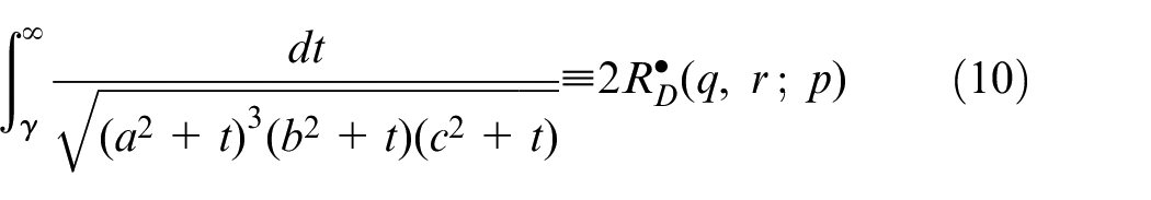
For the S&H solution (and ours) depends on the Thomas & Hoersch integrals , declared by S&H to be elliptic integrals, as indeed they are. Thus
and is just the third permutation of the same three parameters. The Carlson forms above are immediately found (just set ) from the integrals in the form in which they first appear in T&H’s analysis.
But are not “Legendre elliptic integrals”: while is indeed just the difference of two Legendre integrals, and are each the sum of one or two Legendre integral integrals and algebraic terms. To derive them T&H begin by setting : then (dropping a factor ) ; (the relation to the Hertz problem is now lost). They then find (laboriously)
two apparently unrelated equations, which cannot immediately be checked.
Unfortunately, the elliptic integrals are only a part of the solution, and are accompanied by a “tail”: our or S&H’s , which are complicated “elementary” quantities. It is not clear how the very different expressions are related, but numerical tests (but using our forms for ) establish that the answers are the same (A different form of the Sackfield and Hills equations for the full stress distribution is given by Hills et al.,6 from which the tail for the stresses on the plane may be abstracted. But our attempt to evaluate this gave impossible answers). So equations for the subsurface stresses have been available since 1983. What is new, is that the derivation of our equations is given; and that for the first time the stresses have been evaluated and plotted, so that the (minor) distortion of the stresses under a circular contact by the ellipticity may be seen and evaluated. The undoubted easing of the calculation of the elliptic integrals is somewhat offset by the existence of the “tails,” although we would claim that our tail is the simpler.
And indeed, with a computer program capable of complex arithmetic, the need to distinguish between and finally disappears: we found (using MATLAB) that the single equation (A5) does produce the same answers as the alternative two real equations (A6) and (A5b).
Conclusion
The simple, direct, link between the equations for the stresses underneath an elliptical Hertzian contact and (readily calculable) Carlson elliptic integrals has been used to obtain equations for the stresses in the principal planes, while avoiding the distinction between major and minor axes. The stresses along the axis of symmetry, well known from the work of Thomas and Hoersch,5 are now given by a single (simpler) equation, in which “a” and “b” appear on an equal basis. Away from the axis of symmetry, the equations for the stresses involve both elliptic integrals and a long “tail” of complicated elementary functions. The considerable gain from using the immediately obvious, neatly matched, Carlson integrals instead of the rather messy transformation into non-matching incomplete Legendre integrals is diluted by the existence of the tails, though we would argue that ours is the simpler. The final numerical answers are the same as those obtained from the equations given in 1983 by Sackfield and Hills, now for the first time evaluated: but our equations are complete with a derivation.
Maps of the principal stresses and for a typical elliptical contact () are presented. These are much as might be guessed from a knowledge of the stresses under a circular contact, but some differences are noted, particularly when the stresses in the plane of the minor axis are compared to those in the plane of the major axis.
Sadly, the interchangeability of a and b in the elliptic integrals is not maintained in the tails.
The tail for the stresses in the plane of the major principal axis contains a term in arctanh (or a logarithm): the corresponding term in the tail for stresses in the minor principal plane is an arctan. But this was there already in the equations for the surface stresses, and so unavoidable.
Footnotes
Appendix 1
Appendix 2 (crib)
For y = 0 plane
(5) Find:
(6) Find:
where, defining ,
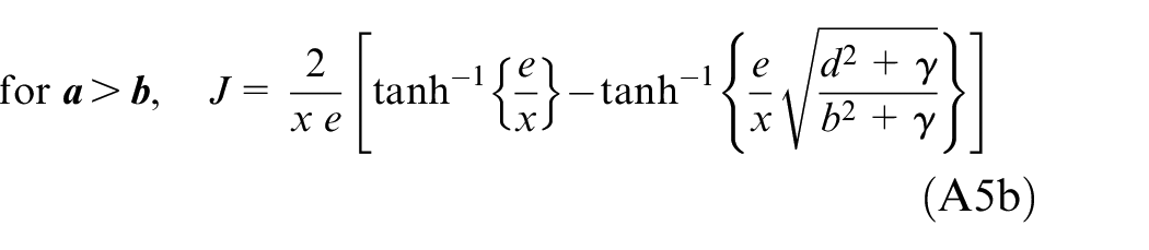
for a > b
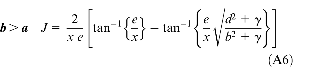
but for b > a
Limiting values as
Declaration of conflicting interests
The author declared no potential conflicts of interest with respect to the research, authorship, and/or publication of this article.
Funding
The author received no financial support for the research, authorship, and/or publication of this article.
ORCID iD
JA Greenwood
References
1.
Love AEH. Mathematical theory of elasticity. 3rd ed.Cambridge: CUP, 1920.
CarlsonBC. Elliptic integrals. Digital library of mathematical functions (DLMF) chapter 19, http://dlmf.nist.gov/ (2010).
4.
GreenwoodJA.Hertz theory and Carlson elliptic integrals. J Mech Phys Solids2018; 119: 240–249.
5.
ThomasHRHoerschVA.Stresses due to the pressure of one elastic solid upon another. Bull. Engng. Exp. Station No. 212. Champaign, IL: University of Illinois, 1930.
6.
HillsDANowellDSackfieldA.Mechanics of elastic contacts. Oxford: Butterworth-Heineman, 1993.
7.
FesslerHOllertonE. Contact stresses in Toroids under radial loads. Br J Appl Phys1957; 8: 387–393.
8.
SackfieldAHillsDA. Some useful results in the classical Hertz contact problem. J Strain Anal Eng Des1983; 18(2): 101–105.