The validation of a full-field deformation analysis of an aircraft panel: A case study

Abstract

The increased use of optical measurement techniques in industrial environments has the potential to increase knowledge and creates an opportunity for a more comprehensive validation of computational predictions. In this paper, a quantitative validation methodology is applied to a 1 m × 1 m panel from an aircraft fuselage subject to compression and torsion, in order to evaluate the predicted response of the panel. A test matrix with four loading cases, namely pre-buckling and post-buckling compression with and without torsion, was used to demonstrate the capabilities of the validation methodology on the industrial component. The out-of-plane displacement fields were analysed with the aid of image decomposition and a validation process was successfully performed using a quantitative metric. The feature vectors, obtained through image decomposition, representing the surface curvature of the physical and virtual specimens were analysed to assess the similarity of the component’s overall curvature. Then, the feature vectors representing measured and predicted displacements for the four loading cases were used to analyse the deformed shapes and conduct a validation process for the simulation outcomes. The predictions of the deformation of the fuselage panel were found to have a high probability of representing the measured data.

Introduction

A comprehensive verification and validation process is key in developing credible engineering models and building confidence in their predictions. In this context, a verification process is implemented first to assure accurate mathematical representation of the relevant physics in the model, which is then followed by a validation process to evaluate the predictions of the simulation from the perspective of the intended use of the model. ¹ Along with the process of building confidence in the model’s predictions, model calibration activities can also be undertaken, the aim of which is to adjust model parameters to improve agreement between the simulation results against a specified benchmark. The current paper focuses on the steps and methodologies in the validation process with the aid of a case study.

It is a common practice during the validation process to evaluate simulation outputs against experimental measurements, which is emphasised in the validation guides produced by ASME ¹ and CEN. ² However, there is a lack of consensus on the methodology to compare the predictions and measurements. The choice of the methodology depends on the field of engineering and the type of predictions being evaluated, amongst other factors. Strain and displacement data are typically of interest for models predicting structural behaviour, and optical measurement techniques are being increasingly used to obtain experimental measurement results ³ equivalent to the colour maps of deformation generated as output by a simulation. In the field of solid mechanics, a series of European collaborative research projects, including ADVISE, ⁴ VANESSA ⁵ and MOTIVATE ⁶ have explored the challenges of utilising full-field maps, such as strain fields, and implementing a validation process in an industrial environment. Research activities in the frame of these projects have led to the development of effective tools for processing full-field maps using image decomposition ⁷ and for comparing the outputs using quantitative statistical methods ⁸ at different length scales, that is ranging between small and large scale components.

Over the last decade, image decomposition techniques have been intensively studied to process measured and predicted strain and displacement fields.^7,9–11 The measured fields obtained using an optical measurement technique, such as digital image correlation (DIC), are typically treated as images, and can be visually compared with the corresponding images obtained from a simulation, for example using finite element analysis. However, for a quantitative comparison within the scope of validation, further processing is necessary because the image pairs could have different co-ordinate systems, pixel spacing or colour bars, which does not allow a direct comparison between two sets of data. These differences can be overcome by decomposing both images and obtaining two unique yet equivalent feature vectors that represent the measured and predicted data, while preserving the key information about the deformation of the entire surface and also reducing the dimensionality of the data from the order of 10⁶ to the order of 10² data points. Following image decomposition, the two feature vectors can be directly compared using a validation metric as part of the validation process.

The aim of the current work is to demonstrate the implementation of the data processing and comparison methodologies in a validation process for an industrial case study. In addition to the lack of standardised validation methodologies identified earlier, there is a scarcity in the literature of detailed industrial examples especially for large-scale components. Most of the previously published studies consider small components in laboratory tests or validate predictions only from a particular area measured by strain gauges. A successful application to an industrial component will demonstrate the robustness of the methods and their progression from lower technology readiness levels to higher levels. Moving from controlled laboratory settings and standard test components to large scale industrial components can present challenges in collecting and processing the data. Similarly, the increase in the complexity of the response of an engineering component and the increase in the amount of data to be analysed, present challenges for which the decomposition and comparison methodologies need to be matured and translated from a research laboratory into an industrial environment. This is key to a wider acceptance of these methodologies across industrial sectors. This paper aims to address these challenges by presenting a complete validation case study based on evaluating surface deformation of a 1 m × 1 m aircraft panel subject to compression and torsion.

Testing and simulation of the fuselage panel

A 1 m × 1 m aircraft fuselage panel subject to compression and torsion was used in this case study. The physical component and the corresponding CAD (Computer Aided Design) data were provided by Airbus. The panel consists of riveted sections with a smooth exterior face and assembled with longitudinal and circumferential skin joints on the interior face, as shown in Figure 1.

Figure 1.

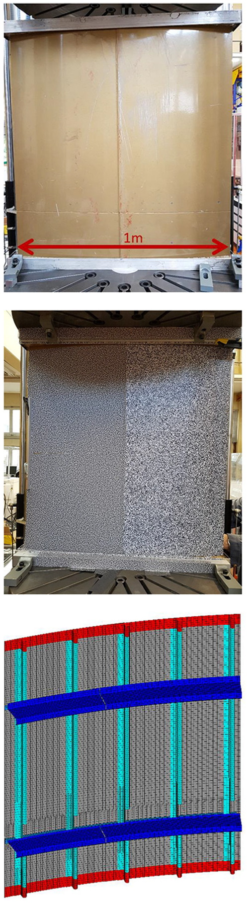
A 1 m × 1 m panel from an aircraft fuselage showing the smooth front face without speckle pattern (top) and with printed speckle patterns (middle) and the corresponding FE mesh (bottom) with equivalent boundary conditions (in red colour). The skin is shown in grey, stiffeners in cyan and frames in blue colour. (For interpretation of the references to colour in this figure legend, the reader is referred to the web version of this article.).

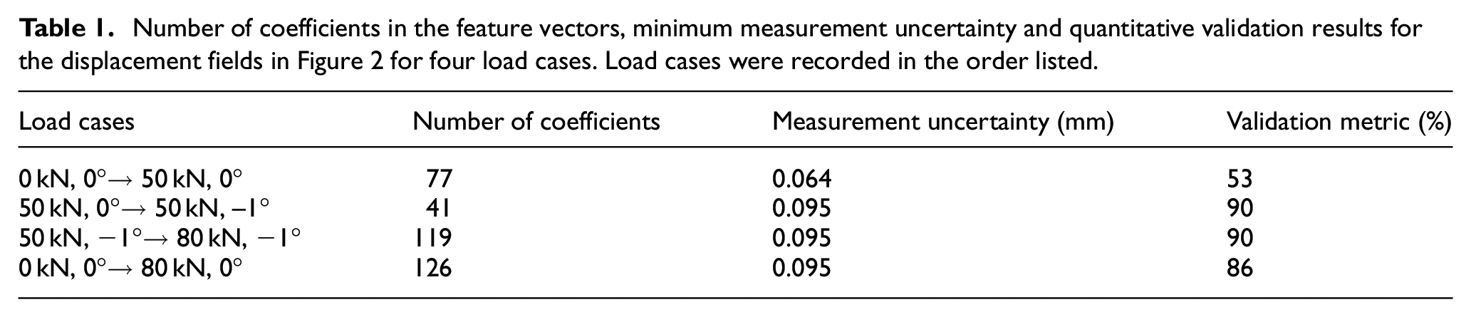
Prior to the physical test, the panel was inspected for any irregularities and damage. No damage was found; however, small geometrical deviations were identified between the CAD model and the real artefact. During its preparation, the edges of the panel were trimmed where necessary to provide a smooth perimeter, and the top and bottom ends were potted in a frame to ensure a secure fit in the test machine and a distribution of the applied load. Speckle patterns printed on self-adhesive vinyl sheets were applied on the front surface, that is the exterior face of the fuselage panel. After the preparation, the panel was mounted in an Instron 1346 test machine and loaded in displacement control. A commercial stereovision DIC system Q-400 (Dantec Dynamics GmbH) was used, consisting of two Baumer VCXG 51M cameras with 2448 × 2048 pixel resolution, 12 mm Schneider Kreuznach lenses and an HILIS LED illumination unit. The DIC system was set-up at 1.9 m from the panel and the cameras were 0.64 m apart. A calibration was performed to establish the minimum measurement uncertainty, u_calibration and the values are reported in Table 1. A novel two-step calibration approach was utilised, which combines a standard DIC calibration process with an additional step to account for the sources of error arising from the test set up. The second step is based on assessing a rigid-body translation between the DIC system and the test component. Further details of the experimental set up and the calibration procedure can be found in Siebert and Splitthof. ¹² The data captured was evaluated using a facet size of 23 × 23 pixels and a pitch of 17 pixels. The measured data fields were stored in an .hdf5 file format during the measurement process.

Table 1.

Number of coefficients in the feature vectors, minimum measurement uncertainty and quantitative validation results for the displacement fields in Figure 2 for four load cases. Load cases were recorded in the order listed.

Load cases	Number of coefficients	Measurement uncertainty (mm)	Validation metric (%)
0 kN, 0°→ 50 kN, 0°	77	0.064	53
50 kN, 0°→ 50 kN, –1°	41	0.095	90
50 kN, −1°→ 80 kN, −1°	119	0.095	90
0 kN, 0°→ 80 kN, 0°	126	0.095	86

A numerical model representing the fuselage panel was developed in the commercial code ANSYS. The panel was represented using shell elements of type ‘shell63’, except for the bolts and rivets which were modelled using rigid beam elements of type ‘beam4’. The resulting finite element mesh is shown in Figure 1. After a mesh convergence study, the average element edge size was set to 10 mm, resulting in 31,740 nodes, 30,220 shell elements and 1198 beam elements. All translational degrees of freedom were constrained at the upper and lower edges of the panel (red elements in Figure 1), except for the displacements in the loading direction at the lower moving edge. The compressive load was applied by gradually increasing the displacement at the nodes located at the lower end of the panel. The predicted data fields were saved as .png files for the validation process.

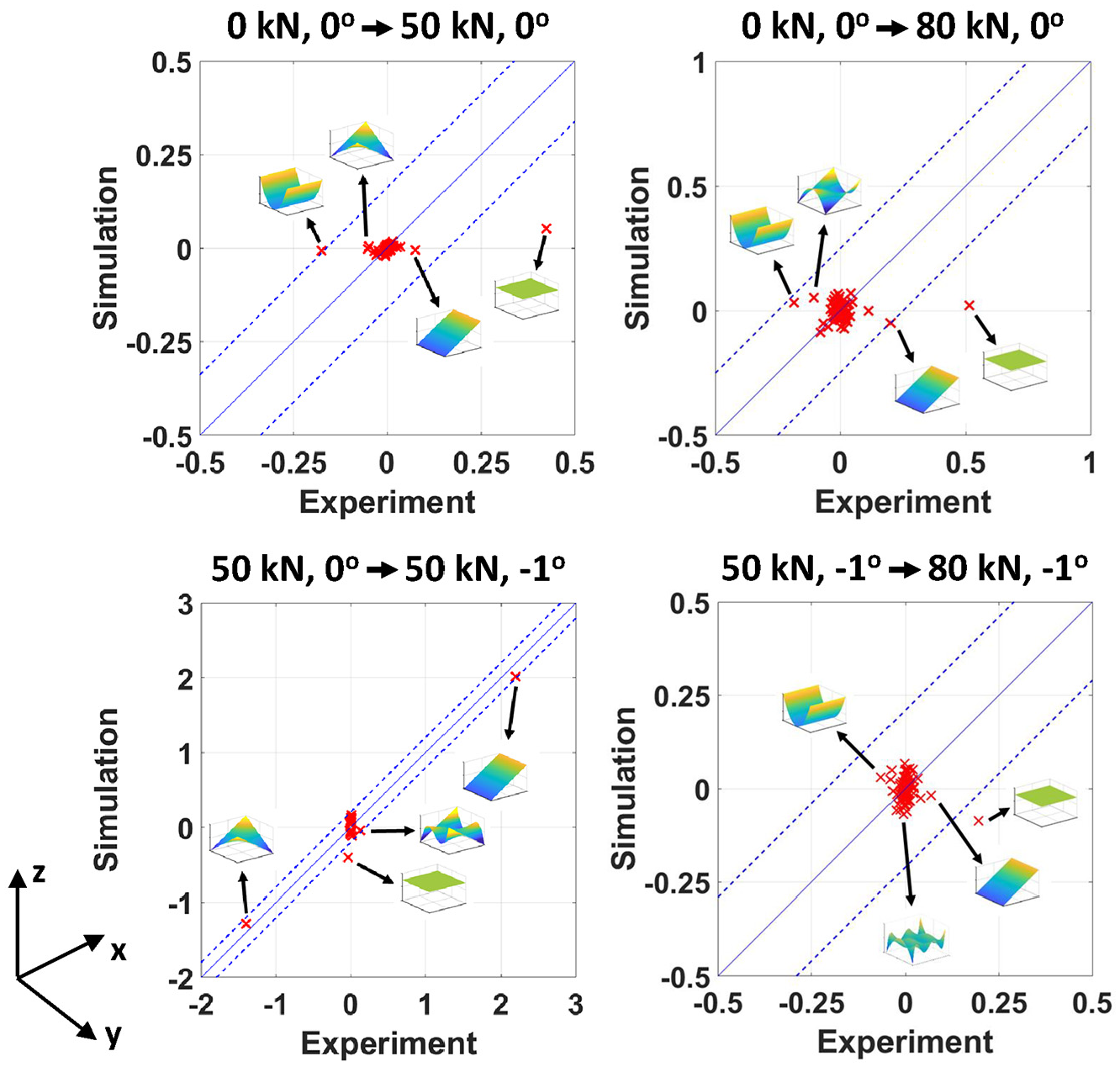
Measured and predicted displacement fields were obtained for four load cases, namely pre-buckling and post-buckling compression with and without torsion. Only one panel was available and so it was not possible to determine its buckling load by experiment in advance of the tests; hence, values of 71.9 kN and 80 kN were calculated using the simulation and buckling theory respectively and used as a guideline. The four data sets were captured during the test at the following stages:

1. From 0 kN to 50 kN in compression;

2. From 50 kN at 0° to 50 kN at −1°, that is a torsion of 1° was applied in the counter-clockwise direction at a constant load of 50 kN;

3. From 50 kN at −1° to 80 kN at −1°, that is a compressive load was increased from 50 kN to 80 kN at a constant torsion angle of −1°;

4. From 0 kN to 80 kN in compression.

The counter-clockwise direction was defined looking from the bottom to the top of the panel, and in the last case, the loading was applied continuously between 0 kN to −80 kN. The measured displacement fields were computed using pairs of DIC images captured at the beginning and the end of each stage, that is reference and object images respectively. For example, for the second load case a pair of reference images were captured at 50 kN and 0° angle of torsion, and the loaded state was captured at 50 kN and −1° angle of torsion. The data was collected over two tests performed on two consecutive days and the calibration was performed on each day to take into account any changes to the experimental set-up and the environmental conditions. Specifically, the panel was unloaded between the first and the second load case, thus two values for the minimum measurement uncertainty were obtained and reported in Table 1. The measured and predicted displacement fields are presented in Figure 2.

Figure 2.

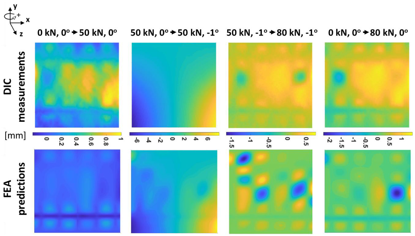
Measured (top) and predicted (bottom) out-of-plane z displacement fields for the aerospace panel in Figure 1 subject to compression and torsion. The four load cases correspond to pre- and post-buckling of the panel, and a negative angle corresponds to counter-clockwise direction of the applied torsion.

Validation methodology

Image decomposition

The displacement and strain fields obtained from the simulations and the optical measurements are typically presented and compared as images. Instead of a visual, essentially qualitative and subjective, side-by-side comparison of such deformation data, it has been previously proposed to utilise image decomposition to process the data from both experiments and simulations to support model updating ¹³ and later for validation.^10,14 By treating a data field, for example a displacement field, as an image in which the magnitude is represented by a colour or grey level value, image decomposition techniques can be easily applied to both simulation and experimental outputs. Image decomposition is a form of orthogonal decomposition based on the principle of fitting a set of selected orthogonal polynomials to an image and is commonly used to both compress data and to identify shapes or features in images for applications such as object tracking, face and natural structures recognition. ¹⁵ A number of different polynomials are described in the literature on decomposition techniques; however, in this case study, Chebyshev polynomials were used because they are discrete orthogonal polynomials defined in a Cartesian coordinate system on a rectangular domain and because of previous experience of their application to engineering exemplars. Not only does decomposition using polynomials reduce the dimensionality of the data, that is from an image that is defined by a two-dimensional matrix to a one-dimensional feature vector, it also provides a unique way of transforming the data from different sources and in different co-ordinate systems into the same format ¹⁶ because the process is invariant to rotation, scale and translation. In addition, information-preserving shape descriptors, that is coefficients of the polynomials, are generated which allow the outputs from simulations and experiments to be compared directly when they are decomposed using the same set of polynomials.

Each of the coefficients in the feature vector corresponds to a specific shape in the image, and the magnitudes of the coefficient corresponds to the prominence of that shape in the image, as shown in Figure 3 for the kernels of the first fifteen Chebyshev coefficients. Following the decomposition of displacement fields, individual coefficients can be analysed and compared to extract further information about, for instance, the curvature of a specimen or a dominant deformation shape.

Figure 3.

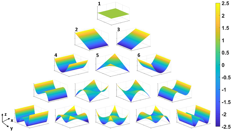
An illustration of the shape of the first fifteen kernels of the Chebyshev polynomials.

In this case study, decomposition was performed using the ‘Euclid’ decomposition tool, ¹⁷ which is available to the public and was developed as part of the EU H2020 project, VANESSA. ⁵ The measured and predicted displacement fields were imported and decomposed separately for each load case over a common region of interest using a large number of coefficients, for example 200. It has been previously shown in Lampeas et al. ¹⁸ that the data sets can be further condensed by removing coefficients with smaller magnitudes, that is removing coefficients that do not significantly contribute to the shape of a data field. This approach was employed here by applying a percentage threshold to obtain four pairs of feature vectors containing only coefficients with significant values; for example, removing coefficients whose magnitude was below 5% of the absolute magnitude of the largest coefficient in the feature vector. 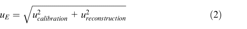The quality of decomposition was assessed against the criteria recommended by the CEN validation guideline ² to ensure that the resulting feature vector accurately represented the original data. The recommended criteria state that the average squared residual, $u_{\mathrm{reconstruction}}$ between the reconstructed and original images must not be more than the minimum measurement uncertainty in the measured data, that is $u_{\mathrm{reconstruction}}<u_{\mathrm{calibration}}$ , and that there should be no cluster of data points in the data field, where the residual is greater than three times the average squared residual. A cluster is defined as a region of adjacent pixels in the image corresponding to more than 0.3% of the image. When some of the criteria are not met, the number of coefficients needs to be increased. The number of significant coefficients in the four feature vectors used for the validation is summarised in Table 1. In the present study, it was not always possible to satisfy all three criteria when decomposing the simulation data due to artefacts in the image files; in such circumstances it was ensured that at least the $u_{\mathrm{reconstruction}}$ criteria was satisfied, as it is further used as part of the validation criteria, and that the measurement data satisfied all three criteria. Once satisfactory decomposition results were obtained, they were exported in .mat format for further analysis. The exported information includes not only the feature vector, but also the reconstructed image and the reconstruction uncertainty.

Validation metrics

The CEN validation guideline ² also provides a methodology for comparison of the feature vectors for the purpose of validation. The methodology is based on plotting the coefficients of the feature vector representing the measured data, $S_E$ against the coefficients of the feature vector representing the predicted data, $S_M$ and graphically comparing the deviations against the uncertainty limits defined by

$$S_E=S_M\pm 2u_E$$

(1)

where $u_E$ is the total measurement uncertainty in the measured data, which comprises, at least, of the minimum measurement uncertainty and the reconstruction uncertainty:

$$u_E=\sqrt{u_{\mathrm{calibration}}^2+u_{\mathrm{reconstruction}}^2}$$

(2)

The CEN methodology was implemented in this case study for all four load cases to make an initial comparison and to visualise the discrepancies between measured and predicted displacement fields. This methodology allows a qualitative comparison of displacement fields, but does not lead to a quantitative validation outcome.

Dvurecenska et al. ¹⁴ have recently proposed a validation metric that extends the CEN methodology and quantifies the similarities between predicted and measured responses. The metric is based on evaluating relative errors, $e_k$ between the components of two feature vectors against a threshold, $u_{\mathrm{threshold}}$ such that

$$\mathrm{VM}={\sum }_i{w}_i{\Vert }_{e_k<u_{\mathrm{threshold}}}$$

(3)

where VM is a weighted sum of errors that are below the threshold, while $w_i$ is the error relative to the sum of the errors expressed as a percentage and the $u_{\mathrm{threshold}}$ is usually taken as the normalised total measurement uncertainty $u_E$ , as in equation (2). ‖ is an indicator function that takes a value of 1 when $e_k<u_{\mathrm{threshold}}$ , otherwise it has a value of 0. As a result, a probabilistic statement about the quality of predictions can be made based on the VM.

Results and discussion

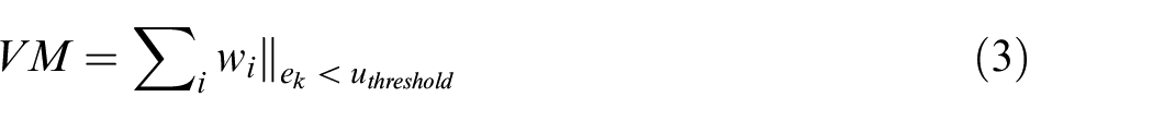
Prior to validation, in addition to the initial comparison of the geometric details in the physical specimen and the numerical model, the global curvature of the panel was evaluated using digital image correlation to measure its shape and utilising image decomposition to assess the difference between the specimen and model. The results are illustrated in Figure 4 and confirm the panel’s initial curvature around its vertical axis as shown in Figure 1. For a more detailed and quantitative comparison of the curvature of the model and the physical panel, corresponding out-of-plane measurements were decomposed. By employing image decomposition, both data sets were translated into equivalent format and the details of the curvature were studied further by analysing individual coefficients of their feature vectors. The difference between the two feature vectors was then calculated and the resulting feature vector was reconstructed to visualise the difference in curvature; this is illustrated in the bottom image in Figure 4. It is evident that, for the majority of the area of the panel, the curvatures are very similar, apart from towards the top edge where the radius of curvature is smaller in the numerical model. This localised discrepancy probably arose during disassembly of the panel from the aircraft or during transportation to the test lab. However, it was considered to not be substantial relative to the overall dimensions and geometry of the panel, and it was agreed to proceed to the validation of the displacement predictions.

Figure 4.

The initial out-of-plane curvature of the aerospace panel in Figure 1 obtained by measurement using DIC (top) and from the CAD data used to generate the FEA model (middle), together with the plot of the absolute difference (bottom) between the two out-of-plane geometries. All dimensions are in mm.

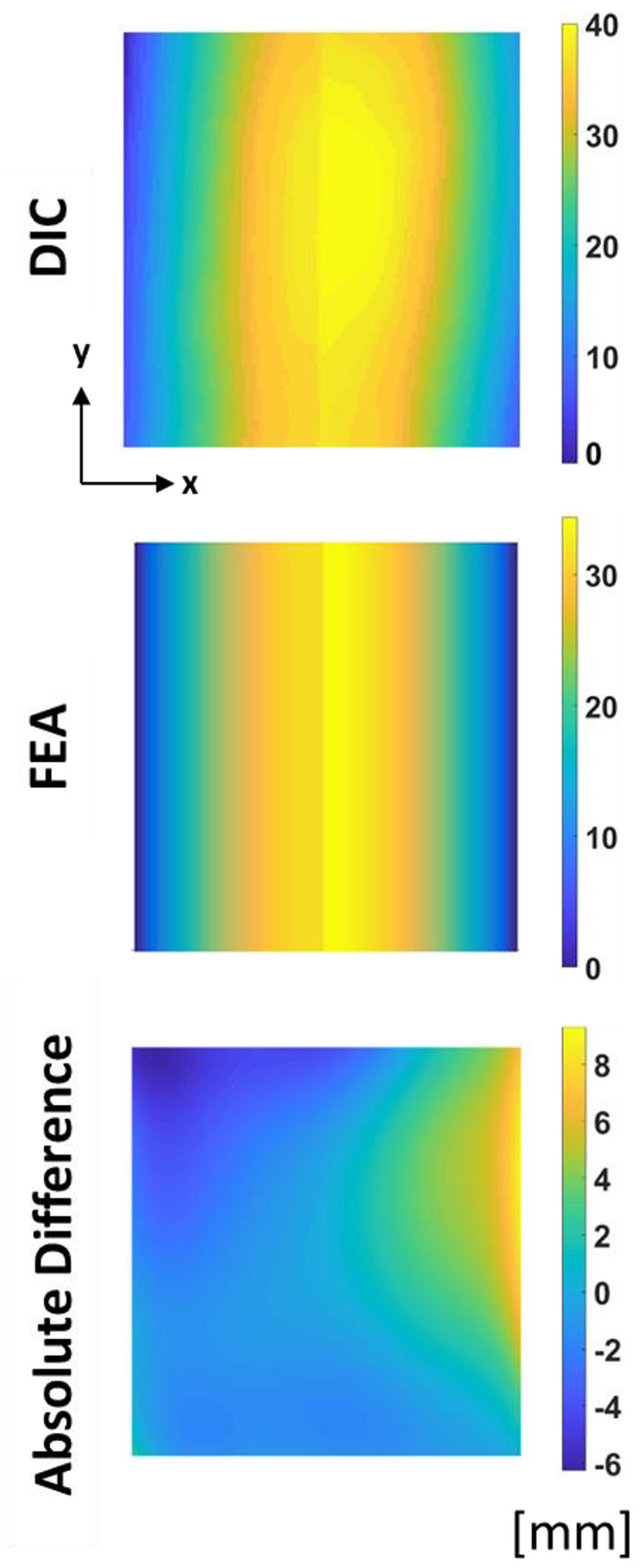
An initial comparison between the measured and predicted data fields was performed using the CEN methodology and the results are summarised in Figure 5. Plotting and evaluating the coefficients with respect to the total measurement uncertainty indicates a number of similarities and differences between predicted and measured displacement fields. Due to the nature of the Chebyshev polynomials, it is possible to explore these similarities and discrepancies further by illustrating the shape of the kernel represented by each coefficient. To illustrate some of the features present in the displacement fields, the four coefficients with the largest absolute magnitude for each load case have been superimposed on the graphs in Figure 5. For example, it can be seen that the fourth coefficient is one of the dominant coefficients in the displacement fields for the 50 kN and 80 kN compression load cases. This coefficient relates to the curvature around the horizontal axis, which clearly corresponds to the dominant shape expected as a result of a compressive load applied along the vertical axis. Also, the third and fifth coefficients are dominant coefficients in the displacement fields representing the 50 kN load case with torsion. These two coefficients correspond to rotation around the vertical axis and bending around the negative x = y line, which were expected to be the dominant shapes due to the torsion around the vertical axis coupled with compression along the vertical axis. The third coefficient can also be related to the initial change in curvature in the physical panel. In contrast to the measured data, this coefficient does not significantly contribute to the description of the predicted data fields in the 50 kN compression load case and in the 80 kN compression load case with and without torsion, that is the magnitude of the third coefficient in the predicted feature vector is much smaller than the magnitude of the corresponding coefficient in the measured feature vector and is very close to zero. Despite this discrepancy between the two data fields, as shown in Figure 4, the third coefficient always falls within the uncertainty limits.

Figure 5.

Plots comparing measured and predicted displacement fields in Figure 2 using the approach described in CWA16779 which involves plotting against one another the coefficients of the feature vectors representing the data fields from the simulation (y-axes) and experiment (x-axes) together with lines representing equality (solid) and equality plus and minus the expanded uncertainty in the measurements (dashed lines). The feature vectors were obtained using image decomposition and the inset kernels illustrate dominant features in the measured and predicted displacement fields. A visual representation of the first fifteen Chebyshev coefficients is shown in Figure 3.

Following the qualitative analysis of the feature vectors, the relative error validation metric was applied to quantitatively compare predicted and measured displacement fields and the results are summarised in Table 1. A relatively low probability was computed for the predictions of the displacement under a 50 kN compressive load. This was expected following the visual comparison of the displacement fields in Figure 2, where it was evident that the simulation underestimates the measured response. This is also supported by the result presented in the top left graph in Figure 5, where the first coefficient is far outside the uncertainty limits indicating unacceptable agreement between predicted and measured results according to the criteria in the CEN guideline. For the other three load cases, namely 80 kN compression and 50 kN and 80 kN compression with torsion, a high probability of the model being representative of the measured data is indicated by the computed VM values. The refinement of the simulation and reconsidering the relevance of the experiment in order to achieve greater congruence between the predictions and experiments is beyond the scope of this study which is focussed on the methods of comparison. However, the information embedded in the Figure 5 concerning which pairs of coefficients are not within the measurement uncertainty could support a diagnosis of the issues causing the lack of congruence.

Implementation of the image decomposition method and the application of the validation metric presented in this paper have demonstrated the depth of analysis that is possible to perform for an industrial case study. Most of the previous studies concentrated on applications in laboratory environments, whereas this paper presents a complete validation case study based on an aircraft fuselage panel. The measured and predicted displacement data fields were fully utilised to interpret the response of a relatively large component and to quantify the discrepancy between measured and predicted responses. DIC was used in this case study to obtain measured data, as it is a common technique used in the aerospace industry during structural testing. However, the methodologies presented in this paper are applicable to a variety of data sets obtained by other measurement techniques, provided that the data can be presented as a map or an image.

Conclusion

A detailed demonstration of a quantitative validation process to an industrial component was presented. The case study was based on evaluating the predicted deformation of a 1 m × 1 m aerospace panel subject to compression and torsion. A more in-depth analysis of the fidelity of the model’s behaviour was achieved through the application of image decomposition and a quantitative validation metric, in comparison to previous validation studies. The validation process presented here included compressing the data fields into feature vectors without losing the key information, and then quantifying the similarities between the predicted and measured responses by comparing the corresponding feature vectors. Individual components of the feature vectors were further studied to identify the dominant shapes of the deformation which contributed to the similarities and differences between the predicted and measured responses. A series of validation outcomes for four load cases were obtained, and it was found that predictions of the deformation of the fuselage panel generally have a high probability of corresponding to the measured data.

The methodologies and the steps described in this paper demonstrate a successful translation of laboratory research into the industrial environment. The validation process that was implemented in this aerospace case study is based on recently published CEN Workshop Agreement (CWA 16799:2014) ² with addition of a probabilistic validation metric ¹⁴ that allows the relative difference between fields of data to be assessed against their uncertainty. These methodologies and the sequence of steps that constituted the validation process can be employed in other industrial sectors where data can be treated as two-dimensional fields or images and the simulations are used for critical decision making. They have the advantages of utilising the entirety of fields of measurements and providing a quantitative evaluation of the extent to which a simulation represents a physical experiment which is the essence of a validation process.