
Abstract
In vibration experiments demanding long-duration measurements, traditional point-wise techniques are often employed, despite the availability of high-speed digital image correlation. This is due to the high volume of images generated by the latter technique, which limit acquisition times and lengthen post-processing times. In this experimental investigation, it is demonstrated that standard frame rate charge-coupled device cameras yield results for the mean deflected shape of a reinforced aerospace panel subject to a random broadband excitation between 0 and 800 Hz that are not statistically different to those from high-speed cameras. The images from both types of camera were processed using digital image correlation to generate out-of-plane displacement maps, which were then decomposed using Chebyshev descriptors for ease of comparison and to determine the mean deflected shape. The results indicate that, with appropriate sampling rates and durations, standard frame rate charge-coupled device cameras can be used to study broadband random excitation behavior of structures when mean behavior needs to be characterized over long time scales compared to the excitation wavelengths. This is contrary to accepted procedures, but offers comparable accuracy with substantially reduced computational resources compared to using high-speed cameras, as well as effectively unlimited data acquisition periods, which is useful in condition monitoring, for example.
Introduction
Structural dynamics is concerned with the behavior of structures subject to dynamic loading that might arise from a number of sources, both natural and man-made. The knowledge of the dynamic behavior of a structure is often important in its design and changes in its dynamic behavior can be used as an indicator of damage in a structure. 1 Computational simulations can be used to optimize designs, but require validation using experimental data, while damage analysis is usually conducted using measurement data. Empirical data, describing the dynamic or modal behavior of a structure, can be obtained from experimental modal analysis when the measured input to the structure is available and from operational modal analysis when only the measured response or output is available. 2 Hence, once natural or resonant frequencies have been identified, mode shapes can be found when external excitation is applied to a structure at a single, known resonant frequency; however, when subject to random broadband excitation, a structure exhibits a random time-varying response that can be characterized by its mean shape over a time period, that is, mean deflected shape. The latter is the focus of this study.
Traditionally, measurements of deformation have been performed using accelerometers, or strain gauges that must be physically attached to the structure, which is both costly and can modify the performance of the structure, and that provide spatially infrequent, separate point-by-point measurement data, which limits the effectiveness of damage detection techniques. 3 Newer technologies, such as laser Doppler vibrometers (LDVs), do not require contact and, with scanning systems, permit high spatial resolution fields of measurements to be generated; however, the sequential measurements can result in excessive test periods, especially when the region of interest is large. 4 Whereas, stereoscopic digital image correlation (DIC) provides a way to measure the displacement of the entire surface of an object simultaneously. 5
Recent advances and availability of high-speed cameras and computer processing technology have stimulated research into a number of approaches to vibration analysis including forms of stereogrammetry, 6 phased-based motion estimation (PME),7–9 combinations of stereogrammetry and PME, 10 fringe projection, 11 and combinations of fringe projection and DIC. 12 However, high-speed cameras are limited by their memory, typically up to 64 GB, that permit data acquisition at their maximum frame rates for only tens of seconds, which would be insufficient for a long-duration test to acquire the mean deflected shape under random broadband excitation, or to monitor the change in dynamic behavior due to structural degradation, induced by service loads or external sources of damage. In addition, high-speed cameras are very expensive and tend to have a lower pixel count compared to standard low-cost charge-coupled device (CCD) cameras used in machine vision applications. However, such standard cameras can record indefinitely in a proper arrangement with a data storage device; but, they are limited to tens or possibly hundreds of frames per second, that means they cannot be used to provide complete spatiotemporal information about structures vibrating at frequencies beyond 50–100 Hz without deploying a stroboscopic light source to “freeze” the motion, 13 which may not be practical for random excitations. These combinations of advantages and disadvantages thwart the low-cost acquisition of vibration shape data with a high spatial resolution and tracking its evolution during long-duration tests on structures excited by random broadband excitation, because high-speed cameras are fast, but expensive and of lower spatial resolution with limited data storage, while standard cameras are cheap, have high spatial resolution and capable of almost indefinite data acquisition, but at limited frame rates. Hence, the goal of this study was to explore the potential overlap in performance of these two types of camera when applied to the experimental measurement of the mean deflected shape of an aerospace panel subject to random broadband excitation, that is, when not attempting to reconstruct the complete time-varying shape of a structure or its modal shapes, but to characterize its behavior based on its shape averaged over time.
Background
As described in the previous section, there are a number of ways of using cameras to capture information about the deformation of structures. In all these techniques, digital images are acquired and processed to generate information about the three-dimensional deformed shape of the structure of interest. A number of methodologies are available to generate this information; for example, motion magnification2,7 has been used to extract modal shape information in the form of edge profiles, for instance, of wind turbine blades, 14 but needs to be combined with photogrammetry 15 or DIC to provide full-field three-dimensional shape data. 11 However, recently Reu et al. 16 have shown that stereoscopic DIC using high-speed cameras is very competitive when compared to LDV, which they considered as the “gold standard”; hence, stereoscopic DIC was adopted in this study to process the data from both the high-speed and standard cameras. The published literature about the use of high-speed DIC to measure random broadband vibration events is limited, perhaps due to the high cost of purchasing two high-speed cameras and the subsequent effort in processing the images. However, one of the major advantages of DIC is that it does not involve contact, so it can be used in applications where other methods might affect the measured response. One such example is provided by Ha et al., 17 who used high-speed DIC to obtain the mode shapes of a beetle’s hind wing, which is quite small and light (85 mm × 43 mm approximately). They used a random base excitation of 0–400 Hz and measured 2000 frames per second for 2 s; then, the out-of-plane displacement at a point was used to calculate the frequency response function (FRF). Another example is provided by Hagara et al., 18 who used high-speed DIC to calculate fast Fourier transforms (FFTs) for a grid of points on a thin panel excited over a 0–500 Hz range by a loudspeaker and recording 1024 images at 1000 frames per second and then harmonic excitation was employed to obtain mode shapes.
Beberniss et al. 19 used high-speed DIC for the measurement of a panel subjected to flow in a wind tunnel. They were interested in measuring several modes of vibration below 1000 Hz in an approximately 250 mm × 130 mm panel subjected to impingement by a high-speed shock flow. The high-speed cameras recorded at 5000 frames per second, which was approximately 10 times the frequencies of interest, and their 32 GB memory was filled in 21 s with more than 100,000 images. The experiment was conducted over a period of 60 s; so, to capture the entire test period, strain gauges and an LDV were also used. They concluded that the results confirmed the viability of using high-speed DIC for nonlinear dynamic displacement and strain response measurements; however, the mode shapes were constructed from the vibrometer data.
Beberniss and Ehrhardt 20 and later Ehrhardt et al. 21 used a similar setup to capture the nonlinear response of a thin beam driven with a shaker. In these studies, the data at only a few locations were utilized to produce an FRF, which was compared to the results from strain gauges and an LDV. They found that a longer recording time, which provided more images to compute the FRF, lowered the noise floor. This concurs with work of Reu et al., 16 who found it was possible to achieve an effective noise floor of 1/10,000 pixel, which produced a displacement noise floor on the order of 10–50 nm and 0.01–0.02 µε. Wang et al. 22 calculated an FRF from full-field vibration measurements of a car bonnet using orthogonal decomposition of displacement maps23,24 to generate shape descriptors. The car bonnet (hood) liner was subject to a random excitation input in the 0–128 Hz frequency range and the response was measured using a pair of high-speed cameras operating at 300 frames per second for 24 s to acquire 7200 frames. They recognized the appropriateness of utilizing the large amount of data in its totality rather than computing an FRF at a few locations, which could be considered wasteful of the rich data produced by the measurement technique. Therefore, they decomposed the full-field DIC data using adaptive geometric moment descriptors (AGMDs) to construct the FRFs. It was found that reconstructing the data fields using the 20 most significant descriptors provided approximately 97% correlation with the original fields. In this case, 14,000 data points were reduced to 20 descriptors with a compression ratio 700:1 and with minimal loss of information. The frequency response of each of these 20 descriptors was then computed to produce the so-called shape descriptor frequency response function (SD-FRF), and the first 11 mode shapes were constructed from the 20 shape descriptors. Subsequently, Allemang et al.25,26 explored the use of principal component analysis (PCA), based on singular value decomposition (SVD), to perform similar transformations on their data. They concluded that the results obtained from SVD-PCA and orthogonal decomposition techniques were comparable, but the former was more straightforward to implement. More recently, Sebastian et al. 13 have used orthogonal decomposition based on Chebyshev (or Tchebichef) polynomials to compare predicted and measured modal shapes for the aerospace panel used in this study.
It can be concluded that the potential of DIC using high-speed cameras as a measurement system in vibration experiments has been demonstrated and the results shown to be reliable for both modal17,18,22,24 and random16,20,21 excitations. The use of decomposition methods to reduce the dimensionality of the resultant data and enable more straightforward comparisons has also been established.13,25–27 While, recently, Berke et al. 28 have shown the correlation between modal shapes for simple rectangular plates and the kernels of the Chebyshev polynomials used in orthogonal decomposition. Hence, orthogonal decomposition based on Chebyshev polynomials was chosen for use in this study to reduce the dimensionality of the out-of-plane displacement fields measured using stereoscopic DIC. The experimental setup and procedures are described in the next section; but, as a precursor, the principles of the orthogonal decomposition are outlined below.
Wang et al.,
29
and subsequently Patki and Patterson,
30
explored the concept of treating maps of measured or predicted strain fields as images that could be decomposed using standard decomposition techniques. The concept has been used to compare measurements and predictions,
27
and its application in this context is described in the CEN guide for the validation of computational solid mechanics models
31
where Chebyshev polynomials are preferred. Hence, the approach described in the CEN guide was utilized in this study and was identical to that used for an earlier study involving the same panel.
13
The data sets were assumed to be rectangular and discrete so that the shape descriptors of an M × N image describing
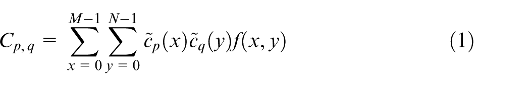
where
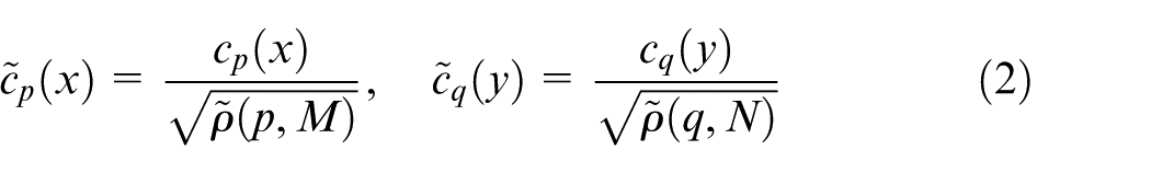
and
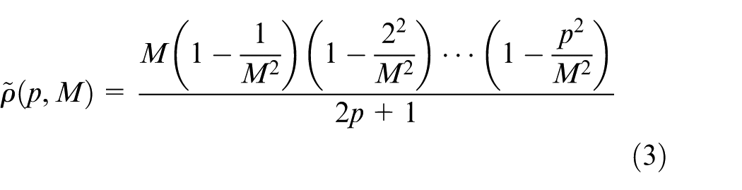
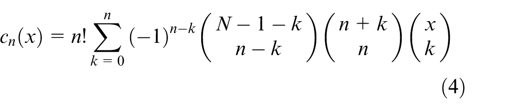
The discrete Chebyshev polynomials are given by
This methodology was implemented in a purpose-written MATLAB code that was originally developed as part of the inter-laboratory study performed during the preparation of the CEN guide. 31 The specifics of its application to the data in this study are described in section “Deflected shape analysis.”
Experimental setup
Data were collected during the random broadband excitation of a prototype aerospace panel using two DIC systems: one system (Q-400; Dantec Dynamics, Ulm, Germany) based on a pair of standard frame rate CCD cameras and the other system (Q-450; Dantec Dynamics, Ulm, Germany) on a pair of high-speed cameras. The 800 mm × 400 mm panel, which had been used in earlier work on modal analysis, 13 was suspended from a portal frame on an optical table, as shown in Figure 1. The detailed geometry for the panel is shown in Figure 2, and the panel has a nominal thickness of 2 mm. The front surface of the panel was machined flat and painted with a random speckle pattern whose size was based on the guidelines provided by Sutton et al. 5 and for which the close-up view is shown in the inset in Figure 2. The back side of the panel has bosses and stiffening ribs machined into it. These can be seen in the bottom of Figure 2. The excitation was provided using a shaker (V100/DSA5-1K; DataPhysics, San Jose, USA) and controller (ABACUS; DataPhysics, San Jose, USA). The controller was used to produce a broadband, random excitation force covering the frequency range of 0–800 Hz.
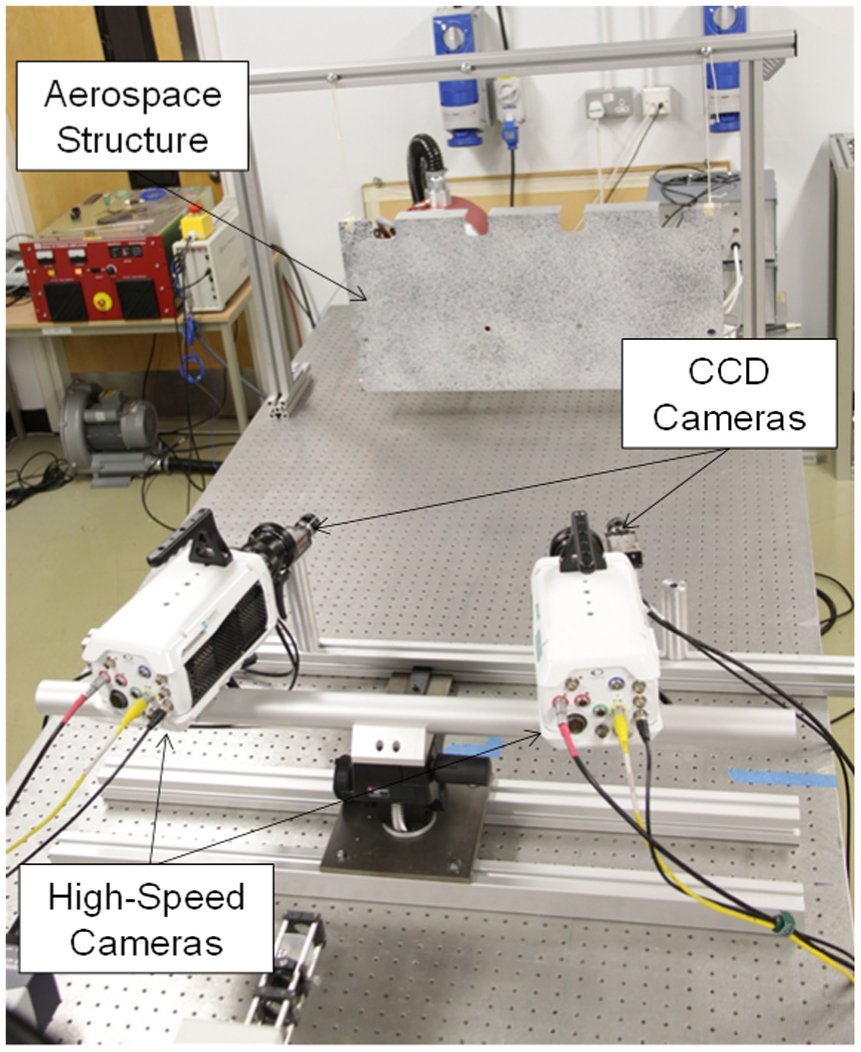
Picture of the experimental setup showing the arrangement of the standard frame rate CCD and high-speed cameras.
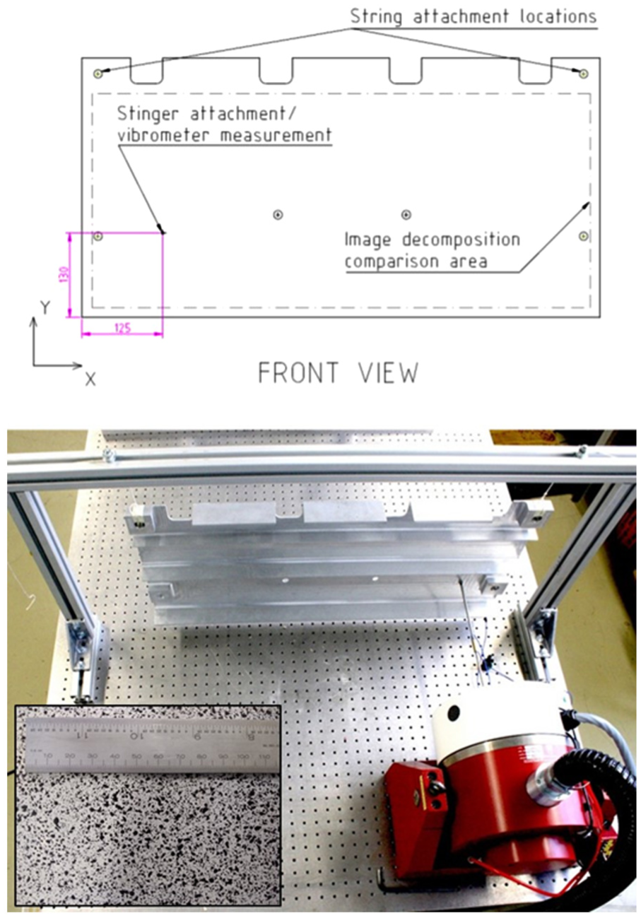
Drawing of the 800 mm × 400 mm aerospace panel showing the attachment and excitation point used in the experiments (top); a photograph of the back face of the panel showing the stinger attachment to the shaker (bottom) and an inset showing a close-up view of the speckle pattern on the front face.
The DIC systems were positioned together on the optical table. The cameras were positioned approximately 135 cm from the panel with a spacing between the cameras of 80 cm producing an angle of approximately 30°. The high-speed cameras, being larger and more cumbersome to place, were positioned on the table first. The CCD cameras were then positioned as close as possible to the high-speed cameras to provide the same angle and field of view of the aerospace panel. The CCD system (Q-400) utilized a pair of FireWire cameras (Stingray F-201 with Sony CCD ICX24 4AL/AQ image device; Allied Vision, Stradtoda, Germany) with a resolution of 1624 × 1234 pixels. A matched pair of 12 mm lenses was used with an f-stop of 1.4. The high-speed system (Q-450) used a pair of CMOS cameras (Phantom v711; Vision Research, Wyne NJ, USA) with a resolution of 1280 x 800 pixels. A matched pair of 35 mm lenses was used with an f-stop of 2.0. Figure 1 shows the physical arrangement of the two camera systems and the aerospace panel during the experiments; Figure 3 shows the control and data acquisition arrangements.
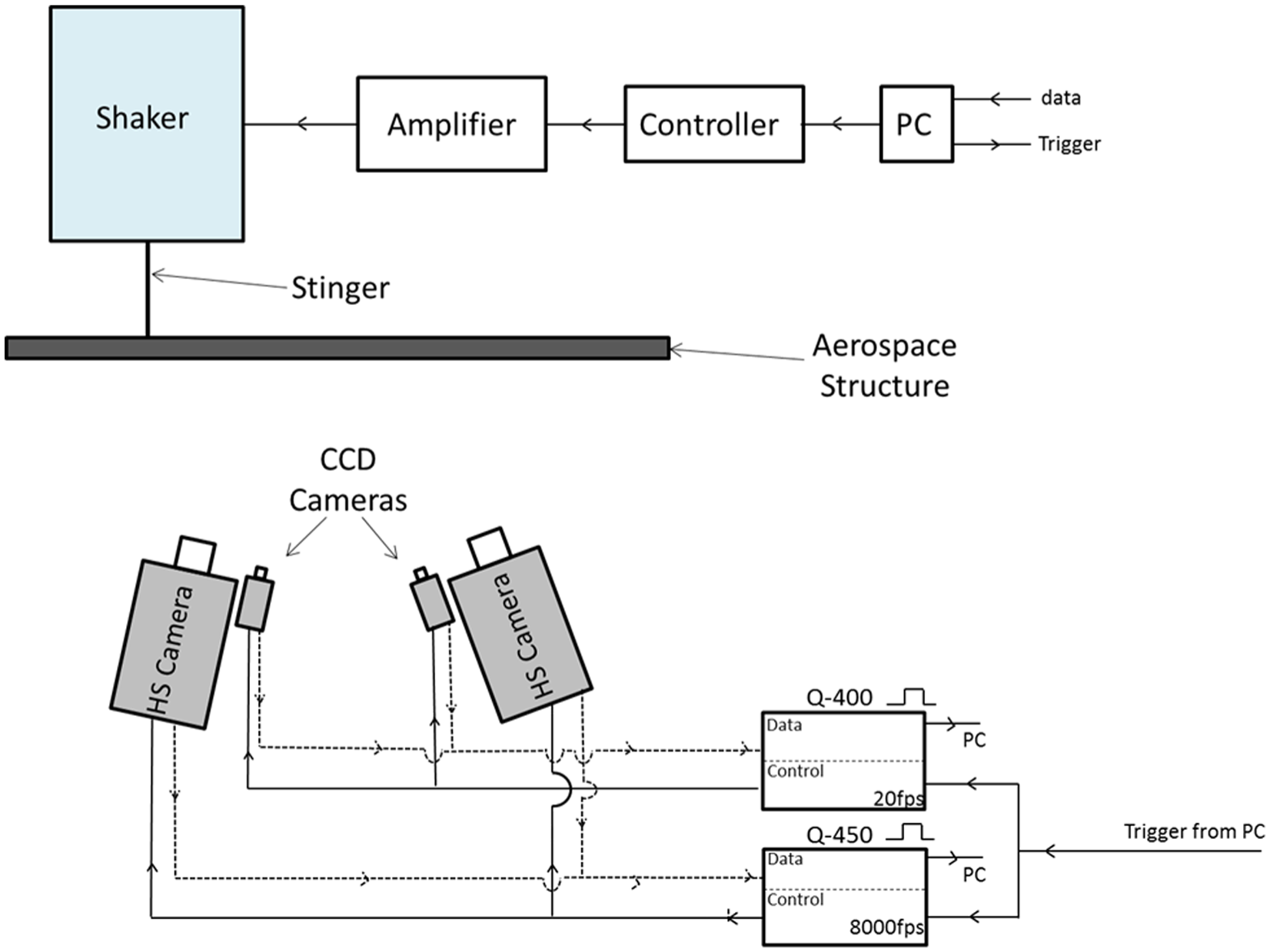
Schematic showing the arrangements for control and data acquisition.
The high-speed cameras were set to record 8000 frames per second, that is, at 10 times the maximum excitation frequency to ensure that the temporal response of the plate was captured, while the CCD cameras were used at their maximum frame rate of 20 frames per second. For the acquisition of the two systems to be in synch, the CCD cameras were triggered at every 400th (=8000/20) image captured by the high-speed cameras. This was achieved using the timing boxes supplied with the standard and high-speed DIC systems. The high-speed timing box output pulses at 8000 Hz were used to trigger the two high-speed cameras. This signal was also routed to the timing box for the CCD cameras, where it was down-sampled to a 20-Hz signal using the software provided with the DIC system.
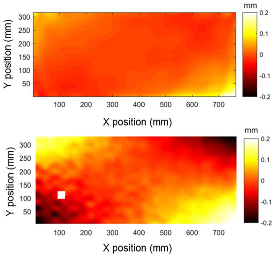
The same experimental setup was used in an earlier study 13 on the same panel, and the FRF from this study is shown in Figure 4 together with the first two modal shapes (14 and 44 Hz) which were obtained using single-frequency sine wave excitation.
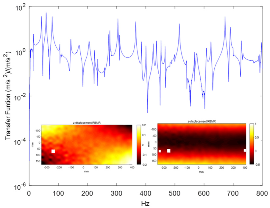
The frequency response function (FRF) for the panel computed using the input excitation provided from the shaker and the output measured by the laser Doppler vibrometer, that is, performing experimental modal analysis; insets are the out-of-plane displacement fields (for the dashed box shown in Figure 2) corresponding to the first two modal frequencies at 14 Hz (left) and 44 Hz (right) with small areas of decorrelation (white).
Deflected shape analysis
The experimental setup described in section “Experimental setup” was used to capture the out-of-plane displacement of the panel using the CCD and high-speed cameras when it was excited by an unknown broadband, random input. The result of the simultaneous measurements was a series of 500 out-of-plane displacement maps based on images from the CCD cameras recorded at a rate of 20 Hz for 25 s and 32,000 out-of-plane displacement maps based on images acquired at a rate of 8000 Hz for a total of 4 s from the high-speed cameras, which was the maximum acquisition time available with memory capacity of the cameras. Hence, only the first 4 s of recording with the CCD cameras corresponded with the data from the high-speed cameras and, at a recording rate of 20 Hz, which corresponded to 80 measurements by the CCD cameras. The captured stereoscopic pairs of images were processed using the DIC algorithm supplied with the systems (Istra; Dantec Dynamics) to produce the full-field maps of out-of-plane displacement. The image magnification was 1.45 and 1.42 pixels/mm, respectively, for the standard and high-speed cameras. The images were processed using 25 pixel subsets with a grid spacing of 21 pixels, which gave arrays of displacement vectors of 53 × 23 and 52 × 23, respectively, for the CCD and high-speed cameras. A flowchart for the processing of the stereoscopic image pairs is shown in Figure 5.
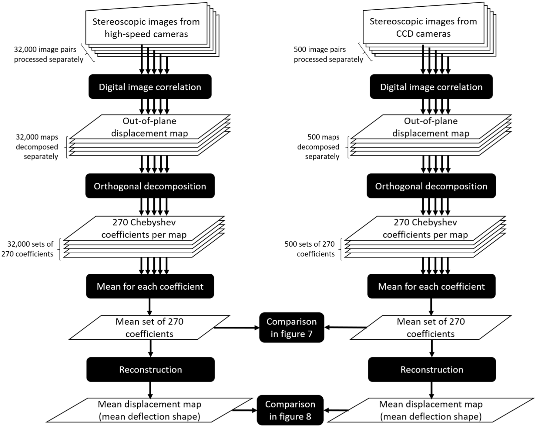
Flowchart showing the processing of the stereoscopic images from the two camera systems obtained during random broadband excitation for 25 s. The CCD cameras recorded 500 image pairs at 20 Hz for the duration of the test, while the high-speed cameras recorded at 8000 Hz for the first 4 s of the test.
The displacement data were decomposed using the Chebyshev descriptors, following the same process described in Sebastian et al. 13 for the same panel subject to modal excitation. The number of shape descriptors used was chosen so that 95% of the displacement fields from the high-speed cameras could be reconstructed to yield a reconstruction error of less than 6%, as shown in Figure 6. The choice of 95% was arbitrary, but the reconstruction error was selected following the CEN guide, 31 which recommends the decomposition process should not introduce errors that are larger than the minimum measurement uncertainty. A calibration process for establishing the minimum measurement error is recommended in the CEN guide 31 and had been used previously to calibrate the same DIC system. 33 The results of this prior calibration established that the minimum measurement errors were 1% and 6% of the maximum out-of-plane displacements in mode 1 and 2, respectively, and hence, the larger value was selected as the mean deflected shape can be considered as a combination of all the mode shapes, thus the highest measurement uncertainty encountered during modal analysis was used in this deflected shape analysis to set an initial criterion for the quality of the decomposition process. To achieve this criterion, 270 descriptors were used, and the resultant reconstruction errors are shown in Figure 6. For each shape descriptor, its mean value was calculated for the 500 out-of-plane displacement fields from the DIC system with the CCD cameras and separately for the 32,000 out-of-plane displacement fields from the high-speed DIC system.
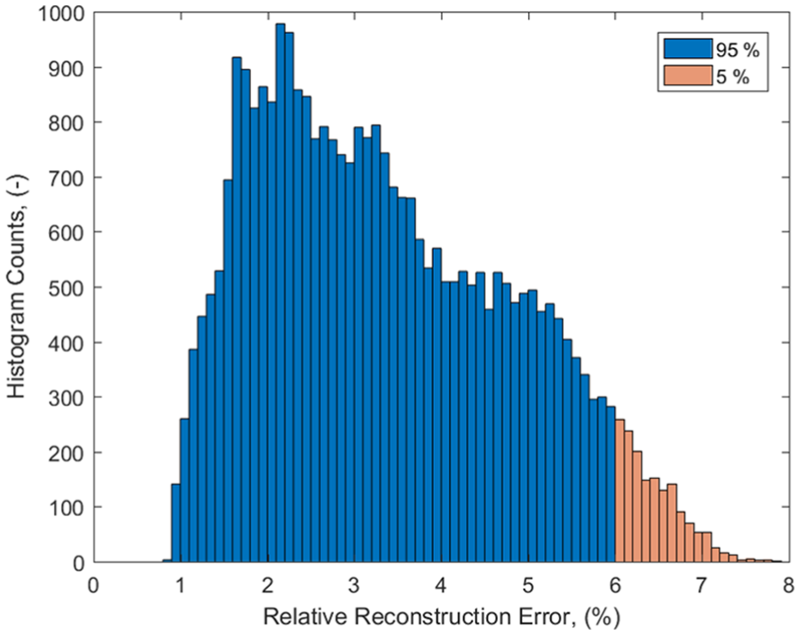
Histogram showing that 95% (dark blue) of the decomposed displacement fields have relative reconstruction errors below 6% for data obtained from the high-speed cameras during random broadband excitation.
Figure 7 shows a scatter plot of the mean Chebyshev shape descriptors, with the data derived from the CCD cameras on the x-axis and from the high-speed cameras on the y-axis. The expanded uncertainty,
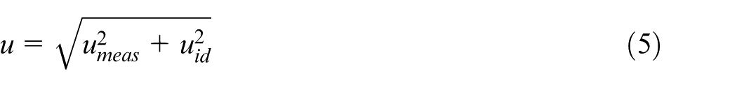
where
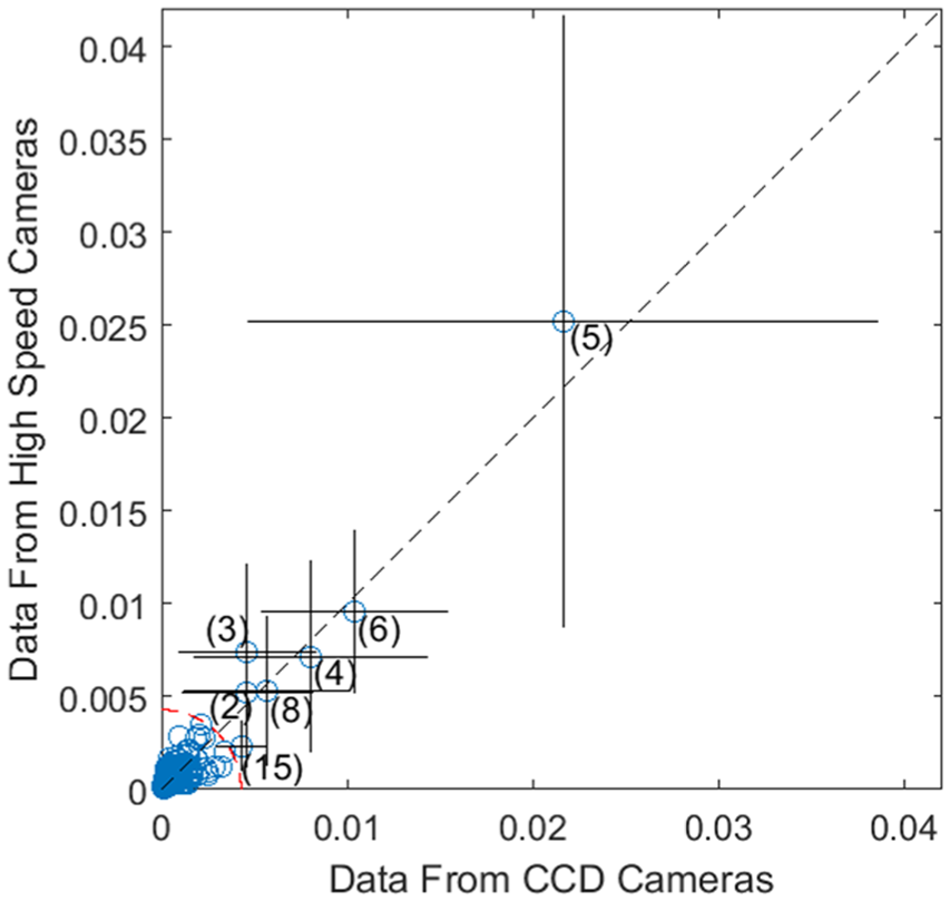
Mean values of the first 270 Chebyshev moments representing the average out-of-plane displacement fields during the data acquisition periods of the high-speed and CCD cameras when the panel was subject to random broadband excitation. Standard deviations are shown as error bars and the unexpanded uncertainty as a quadrant arc in the bottom left.
Discussion
Ideally, all of the data points on Figure 7 should fall on the x = y line, which would indicate that for this metric, the CCD cameras and the high-speed cameras produce the same results. In reality, there will be deviations arising from variations in the data caused by differences in the experimental setup, such as the small differences in viewing angle and magnification, and from the measurement uncertainties. Hence, the data falling within the expanded uncertainty of the measurement systems can be omitted from the comparison, as they fall below the effective resolution capability of the systems. The shape descriptors which have values greater than the expanded uncertainty have been plotted along with the standard deviation of the measurements in Figure 7 beyond the quadrant. This provides information about the variability in the data, and so for those shape descriptors whose error bars of one standard deviation intersect the x = y line, it can be concluded that there is no significant difference between the data from the CCD and high-speed cameras.
Figure 8 shows the mean values of the Chebyshev shape descriptors derived from the data from the CCD and high-speed cameras, along with the reconstruction of the out-of-plane displacement map from those shape descriptors, which represents the mean deflected shape of the panel when excited by random broadband vibrations over the specified frequency range. These two reconstructions appear to be nearly identical, which is highlighted by plotting the difference between the two sets of shape descriptors and the resultant reconstructed map of differences in the bottom of Figure 8. As expected, the mean deflected shape in Figure 8 corresponds closely to the first modal shape, as shown in Figure 9.
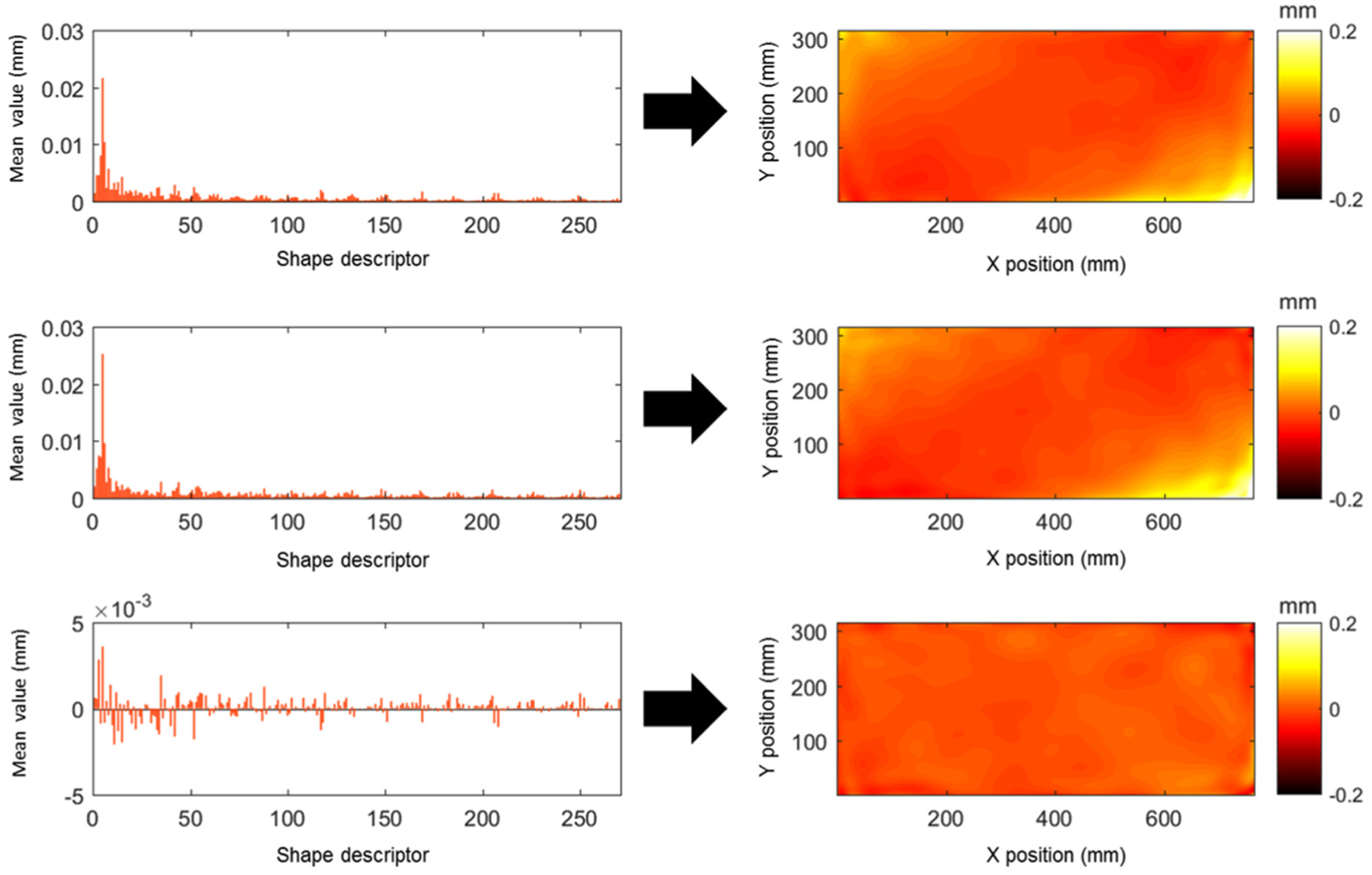
Mean Chebyshev moments or shape descriptors (left) and the corresponding reconstructed out-of-plane shapes or mean deflected shapes (right) for the dashed box in Figure 2 based on the data from the CCD cameras (top), high-speed cameras (middle), and the difference between the two sets (bottom).
The results presented in Figures 7 and 8 imply that CCD cameras can be used in place of high-speed cameras in a DIC system to characterize the overall behavior of a component subject to random broadband excitation, when orthogonal decomposition is used to process the resultant out-of-plane displacement fields to generate the mean deflected shape. In this study, data were collected from the CCD cameras for 25 s, yielding 500 data sets, which the results in Figures 7 and 8 demonstrate is sufficient to represent the mean behavior of the panel; however, this representation will become less reliable with shorter acquisition times and smaller data sets. This is illustrated in Figure 10, in which the Euclidean distance between the feature vectors containing the mean shape descriptors obtained from the high-speed and CCD camera systems is plotted as a function of the number of maps acquired using the CCD cameras. It can be observed that the Euclidean distance between the feature vector obtained using the 32,000 maps from the high-speed system and that obtained using the displacement maps from the CCD cameras decreases as the number of maps from the CCD cameras increases. The Euclidean distance decreases by a factor of almost two when the number of maps is increased from 20 to 500, and when more than 400 maps are used, it is approximately constant at 0.0095 mm, or 4.75% of the maximum out-of-plane displacement in the mean deflected shape, which implies that the number of CCD maps used in this study was sufficient to ensure a reliable measurement. In the range of 135–315 maps, the Euclidean distance is approximately constant at 5.5% of the maximum out-of-plane displacement, which suggests that 140 CCD maps could be used to generate a reasonably reliable result for the mean deflected shape, and this would require data to be collected for only 7 s. Acquiring data in short bursts of around 7 s would allow the degradation of a structure to be monitored for effects that caused a larger than 5.5% change in the mean deflected shape. In general, the required number of displacement maps will be dependent on the frequency range of the broadband excitation, which was from 0 to 800 Hz in this study. When a larger difference of the order of the minimum measurement error, that is, 6%, is acceptable, then the number of displacement maps can be reduced to about one-fifth of the maximum frequency of excitation, assuming the CCD cameras are sampling at 20 frames per second. These limits would have to be scaled appropriately for different CCD sampling rates and perhaps also for maximum excitation frequency, that is, 400 CCD image pairs would be required to define the mean deflected shape, within the minimum measurement uncertainty, for random excitation of a structure between 0 and 2000 Hz using CCD cameras sampling at 20 frames per second.
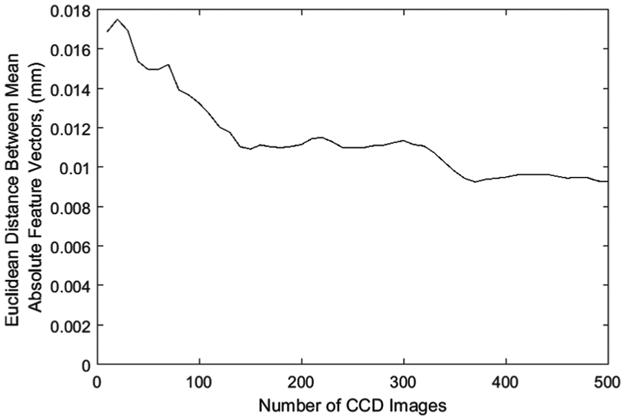
Euclidean distance between the feature vectors containing the mean shape descriptors derived from data from high-speed and CCD cameras as a function of the number of image pairs acquired using the CCD cameras when the broadband excitation is between 0 and 800 Hz, and 32,000 image pairs are acquired using the high-speed cameras.
In this study, 270 Chebyshev coefficients were needed to ensure that 95% of the displacement fields could be reconstructed with an error of less than 6%, which is large compared to the 20 descriptors used in a previous study on the same panel. 13 However, in the previous study, only well-defined modal shapes were decomposed, which could be more easily defined by the Chebyshev descriptors than the more complicated shapes induced by broadband excitation in this study. The effect of using fewer coefficients was examined by comparing the resultant reconstructions with those obtained using 500 coefficients, which is equivalent to 40% of the number of data values in each displacement field and hence expected to give a near-perfect reconstruction. The results are shown in Figure 11 for both the mean deflected shapes and the corresponding Pearson correlation coefficients. The Pearson correlation coefficient decays slowly with the reduction in coefficients and is approximately 0.98 for the 270 coefficients used in this study, which is a compression ratio of 4.4. The reconstructions show that reducing the number of coefficients effectively leads to smoothing of the mean deflected shape as the high-frequency components of the shape are no longer represented; however, if this was acceptable, then a compression ratio of 60 could be achieved. This is an issue of elegance rather than computation efficiency because the difference in resources required to decompose with 500 or 270 coefficients is negligible compared to those required for the DIC described below.
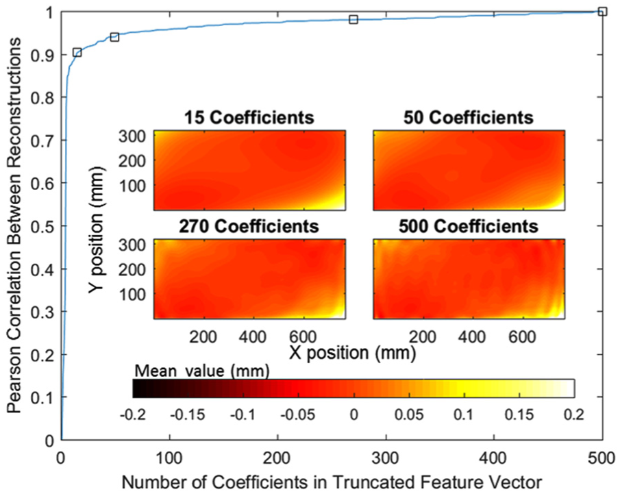
Pearson correlation between the mean deflected shape based on CCD camera data reconstructed using a feature vector containing the full 500 coefficients and the corresponding shapes reconstructed using truncated feature vectors. Four exemplar reconstructions are shown as insets with their corresponding Pearson correlation marked with squares on the graph.
The results from this study imply that high-speed cameras are not always necessary to characterize the behavior of components subject to random, broadband excitation. The mean behavior, in terms of the mean deflected shape, can be obtained using standard frame rate cameras that are capable of effective infinite data acquisition. This capability would allow such a system to be used to monitor the change in behavior of a structure due to operating or material conditions when subject to long-term random broadband excitation, providing the changes occurred at a relative slow rate compared to the excitation frequencies. The instantaneous behavior could also be obtained using CCD cameras combined with a pulsed-laser system triggered by an LDV, as described in previous work. 13 The advantages of not using high-speed cameras include lower cost, physical size as well as data output and processing overheads.
The study represents an advance on machine vision techniques that rely on camera calibration 6 and edge detection algorithms34,35 to evaluate changes in component profile during excitation because the mean deflected shape for the complete component can be obtained. The use of a pair of stereoscopic CCD cameras combined with DIC and decomposition of the displacement fields provides a simpler route to the mean deflected shape than combining PME with DIC or stereogrammetry8–10 and could also provide the FRFs using the approach, based on shape descriptors, as shown by Wang et al.; 22 however, neither PME nor the SD-FRF approach has been demonstrated on long time duration tests with random broadband excitation, as used in this study. The computer resources required for the high-speed DIC measurements of the random nonlinear response of a panel made by Beberniss and his co-workers19–21 were substantial requiring several hours to process 24 s (122,895 frames) of data, 20 and similarly, in this study, the high-speed camera data took about 8 h to process, whereas the data from the CCD cameras were processed in a few minutes on the same computer. Thus, in circumstances where the mean deflected shape needs to be monitored over long time periods, the use of CCD cameras, with appropriate sampling rates and durations, can provide data that is not significantly different from that obtained with more sophisticated and expensive systems.
Conclusion
A method has been proposed to utilize standard frame rate CCD cameras for measuring the mean deflected shape of components during random broadband excitation using, for the first time, feature vectors to determine the mean deflected shape. The out-of-plane displacement fields from a standard stereoscopic DIC system (500 images at 20 Hz) were compared to those from a high-speed system (32,000 images at 8 kHz) by decomposing the displacement fields with the Chebyshev descriptor. It was found that there was no statistical difference between the mean feature vectors derived from the data from the two camera systems. The number of displacement maps required from the CCD cameras, to ensure the differences in the results from the two systems was less than the minimum measurement error (6%), was found to be one-fifth of the maximum excitation frequency. This new finding implies that for long-term recording during random broadband excitation tests, which are not currently possible with high-speed cameras due to difficulties handling and processing the quantities of data generated, it is possible to use CCD cameras to monitor the mean deflected shape of the structure with appropriate sampling rates and durations. This provides the opportunity for low-cost straightforward monitoring of the dynamic response of a structure subject to random broadband excitation, which will enable long-term condition monitoring and the evaluation of evolving boundary conditions on the dynamic response of a structure.
Footnotes
Acknowledgements
The US Government is authorized to reproduce and distribute reprints for governmental purpose notwithstanding any copyright notation thereon. The authors are grateful to Dr Ravi Chona, Structural Sciences Center, US Air Force Research Laboratory, Dayton, OH, and Professor Randy Allemang, University of Cincinnati, for a number of discussions that motivated this study.
Declaration of conflicting interests
The author(s) declared no potential conflicts of interest with respect to the research, authorship, and/or publication of this article.
Funding
The author(s) disclosed receipt of the following financial support for the research, authorship, and/or publication of this article: This work was sponsored by the European Office of Aerospace Research and Development (EOARD) and the Air Force Office of Scientific Research (AFOSR), USAF under grant number FA9550-16-1-0091. Lt. Col. Dave Garner (EOARD) and Dr David Stargel (AFOSR) were the program officers for these grants.