Sage Journals: Discover world-class research

Abstract

In recent years, the number and capability of Synthetic Aperture Radar (SAR) sensors in ow Earth orbit has grown considerably, with multiple commercial satellites now capable of capturing sub-metre resolution imagery. In this study, we present the first application of such very-fine resolution SAR imagery to measure ice velocity of a high mountain glacier. To achieve this, we apply feature tracking to a pair of Capella images in spotlight mode (0.35 m resolution) acquired in July 2021 over Baltoro Glacier in the Karakoram, Pakistan, and compare the results to ice velocities derived from feature tracking using more commonly employed TerraSAR-X Stripmap (3 m) and Sentinel-1 Interferometric Wide (IW) (5 × 20 m) imagery. We show that Capella-derived velocities reveal subtle features that are not evident in velocities derived using coarser resolution imagery. In particular, slower moving ice at the glacier margin, variations in velocity between different flow units, and lateral fluctuations reflecting the local topography are all more clearly resolved. However, the small footprint of the imagery and lack of stable ground within the frame poses a challenge for co-registration, resulting in an inherent, and spatially varying, bias of up to 0.5 m/day in the measured offsets. We reduce this error to ∼0.1 m/day using a global shift and propose that the derived data then show potential to advance knowledge in a range of glaciological disciplines.

Keywords

Synthetic Aperture Radar (SAR)feature tracking ice dynamics sentinel-1 Capella TerraSAR-X

Highlights

1. We apply feature tracking to a pair of Capella images acquired of Baltoro Glacier in July 2021.

2. We compare the feature tracking results with those derived from Sentinel-1 and TerraSAR-X.

3. Velocity data from Capella imagery show detailed ice flow patterns that coarser sensors cannot discern.

Introduction

Mountain glaciers are currently losing more mass than the Greenland and Antarctic ice sheets combined, contributing 27 ± 22 mm/a to global sea level rise (Zemp et al., 2019). Anthropogenic climate change has driven accelerating mass loss (Hugonnet et al., 2021), and altered glacier dynamics (Dehecq et al., 2019) with glaciers in the Himalaya contributing disproportionately to the most recent changes when compared to other glacierized regions worldwide. This trend is expected to continue, with a projected loss of 26–41% of the global mountain glacier mass by 2100, relative to 2015, and up to 71–94% in the eastern Himalaya in particular (Rounce et al., 2023). Runoff from such glaciers provides drinking water, irrigation, and hydropower for millions of people (Pritchard, 2019) but is expected to peak for many catchments in High Mountain Asia around the middle of the century (Huss and Hock, 2018) before declining thereafter. Accurately forecasting how mountain glaciers will respond to climate change necessitates a thorough understanding of their current behaviour, including the various processes that govern the transport and distribution of mass.

Often located in remote locations, in situ measurements of mountain glacier mass balance and ice flow are sparse. In contrast, satellite-based measurements are now abundant, thanks to a growing number of constellations, cloud-based computing, and lengthening image archives. Repositories such as ITS_LIVE (Gardner et al., 2019) and RETREAT (Friedl et al., 2021) contain automatically processed ice flow data derived from openly available satellite imagery and provide the main input into estimations of key glacier parameters, such as ice thickness and ice emergence (Miles et al., 2021; Millan et al., 2022). These ice velocity data are most commonly derived using feature tracking (sometimes referred to as offset tracking or speckle tracking), as the algorithm is relatively simple, such that broad scale analysis of glacier movement can be efficiently implemented (Strozzi et al., 2002). However, because of their broad area coverage, the spatial resolution of available outputs (e.g. 240 m for ITS_LIVE) is necessarily coarse, and thus finer details of the glacier flow field are rarely resolved. Many existing velocity measurements are also derived from optical data that are frequently hampered by the presence of clouds and variable solar illumination (Kääb et al., 2016). On the other hand, SAR, being an active instrument, can penetrate cloud cover and generate its own illumination due to its microwave antenna, thus providing consistently high-quality images suitable for feature tracking. SAR feature tracking offers one further, important advantage – it can track not just physical features on the glacier surface, such as debris, supraglacial ponds, or crevasses, but also speckle patterns, given they maintain coherence between image acquisitions.

The last decade has seen the launch of several commercial SAR satellites (e.g. Capella, Umbra, and ICEYE) which offer sub-metre resolutions and have planned fleets comprising tens of satellites promising short revisit times (Villano et al., 2022). In particular, Capella’s Spotlight mode features a swath width of 5 km at a spatial resolution of up to 0.5 m (ground range pixel spacing of 0.35 m), in contrast to the 250 km swath width and 5 × 20 m resolution of Sentinel-1 (S1)’s Interferometric Wide (IW) mode. Although they do not yet possess a substantial archive of imagery, these commercial image sources promise to revolutionize the detail that can be obtained from mountain glacier surfaces that are normally characterized by only a handful of pixels across the main tongue. Feature tracking has previously been applied to ICEYE data to assess the dynamics of Jakobshavn Isbrae, a large, fast-flowing outlet glacier in Greenland, demonstrating that imagery from these satellites has potential for measuring ice speed (Łukosz et al., 2021). However, their ability to produce robust velocity data at smaller, slower flowing mountain glaciers, where fine resolution is more important, is yet to be comprehensively tested.

This paper aims to fill this gap by applying feature tracking to a pair of sub-metre resolution Capella Images of the Baltoro Glacier separated temporally by just over a week and comparing the results to those obtained from coarser resolution imagery. Specifically, we compare the results from very-fine resolution Capella Spotlight imagery (0.35 m) to those derived from fine-resolution TerraSAR-X (TSX) Stripmap imagery (3 m), and from medium-resolution Sentinel-1 IW (5 × 20 m), both of which are commonly applied in studies of glacier flow (Friedl et al., 2021; Quincey et al., 2009). We highlight challenges around image co-registration for scenes with limited swath extent and present a method for correcting any misalignment, as well as making a quantitative comparative evaluation of images with differing resolution to resolve fine-scale characteristics of glacier flow. The potential for operationalising detailed measurements of glacier flow across broad areas, as the sub-metre SAR image archives lengthen in coming years, is also discussed.

Study area

Baltoro Glacier (Figure 1) is a large (63 km long) debris-covered glacier located in the dry, cold, and high altitudes of the Karakoram mountains. Located at the strategically important intersection of Pakistan, India, and China, the Karakoram mountains provide meltwater and runoff to millions of people within the Indus River basin (Immerzeel et al., 2020). Glacier-driven variability in water supply has historically been a point of conflict between the major powers in this region and has the potential to be reignited in the face of diminishing supplies (Azam et al., 2021).

Figure 1.

Overview map of Baltoro Glacier, showing the outline of the main glacier and its tributaries (in red), as well as nearby mountain peaks (green triangles). The footprint of the Capella scene used in this study is outlined in blue. The background image is a true colour composite of optical planet imagery (Planet Labs PBC, 2017) Image © 2017 Planet Labs PBC”.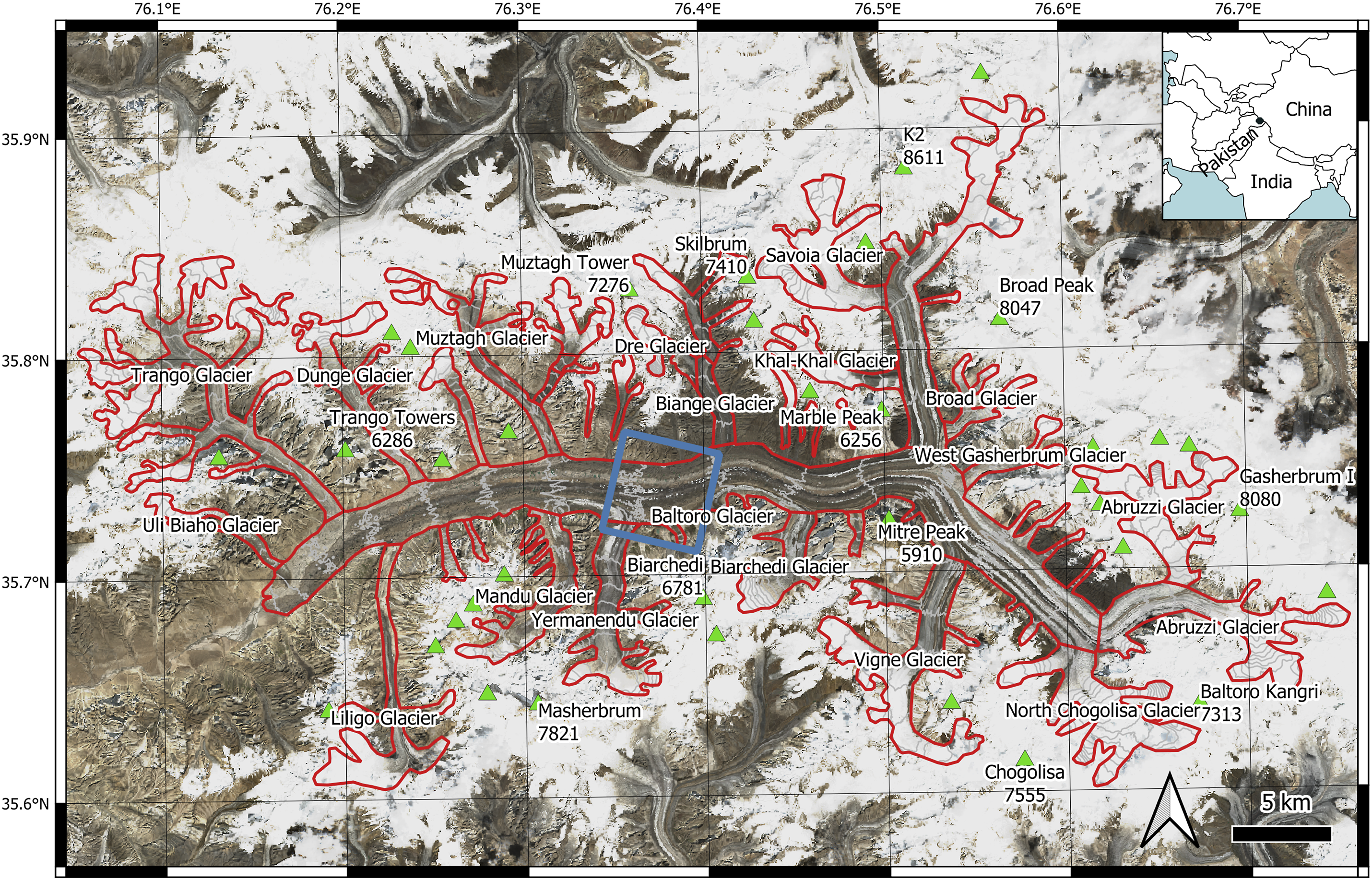

Baltoro Glacier has been relatively well studied, with multiple surveys of glacier velocity from field campaigns and satellite data (Copland et al., 2009; Mayer et al., 2006; Quincey et al., 2009; Wendleder et al., 2018, 2023). These studies show clear seasonal differences in velocity, as well as apparent multiannual cyclicity, perhaps linked to precipitation and supraglacial lake evolution (Wendleder et al., 2018). Baltoro’s surface velocities are known to reach a maximum of around 0.6 m/day at Concordia, the confluence between the Godwin-Austen Glacier and the Baltoro South branches. As commonly observed in mountain glaciers, surface velocity gradually decreases towards the terminus as the ice becomes thinner, with some variability linked to the changing width of the valley and to tributaries adding mass to the main tongue.

The numerous tributaries of Baltoro Glacier have been less studied (Gibson et al., 2017), mainly due to the poor ability of medium-resolution sensors to resolve the dynamics of small, slow-flowing glaciers. Several of Baltoro’s tributaries are known to be of surge-type, including Trango and Muztagh (Paul, 2015).

Baltoro Glacier’s distinct surface is ideal for feature tracking, as its ablation zone is largely covered by debris, which is rich in texture, and pocked with other surface features as it thins from the terminus up-glacier (Mayer et al., 2006) (Figure 2). Numerous supraglacial ponds are present in surface depressions, covering between 3.6 and 5.8 km² of the glacier surface in recent years (Wendleder et al., 2021). Ice sails protrude up to 20 m above the glacier surface (Evatt et al., 2017), and surface streams cut their way across the glacier surface between topographic highs. The topographic highs and lows, brought about by differential ablation (Rowan et al., 2021), also provide a coherent pattern that is ideal for an automated feature matching approach.

Figure 2.

Annotated Capella spotlight image (near full 5 km swath extent) of the central section of Baltoro Glacier captured on 15 July 2021 with inset panels highlighting surface glacial features distinguishable in the SAR imagery. Relatively stable features such as the ice sails are ideal for feature tracking, and the detail captured at the lateral shear margin enables fine-resolution measurements for the velocity gradients.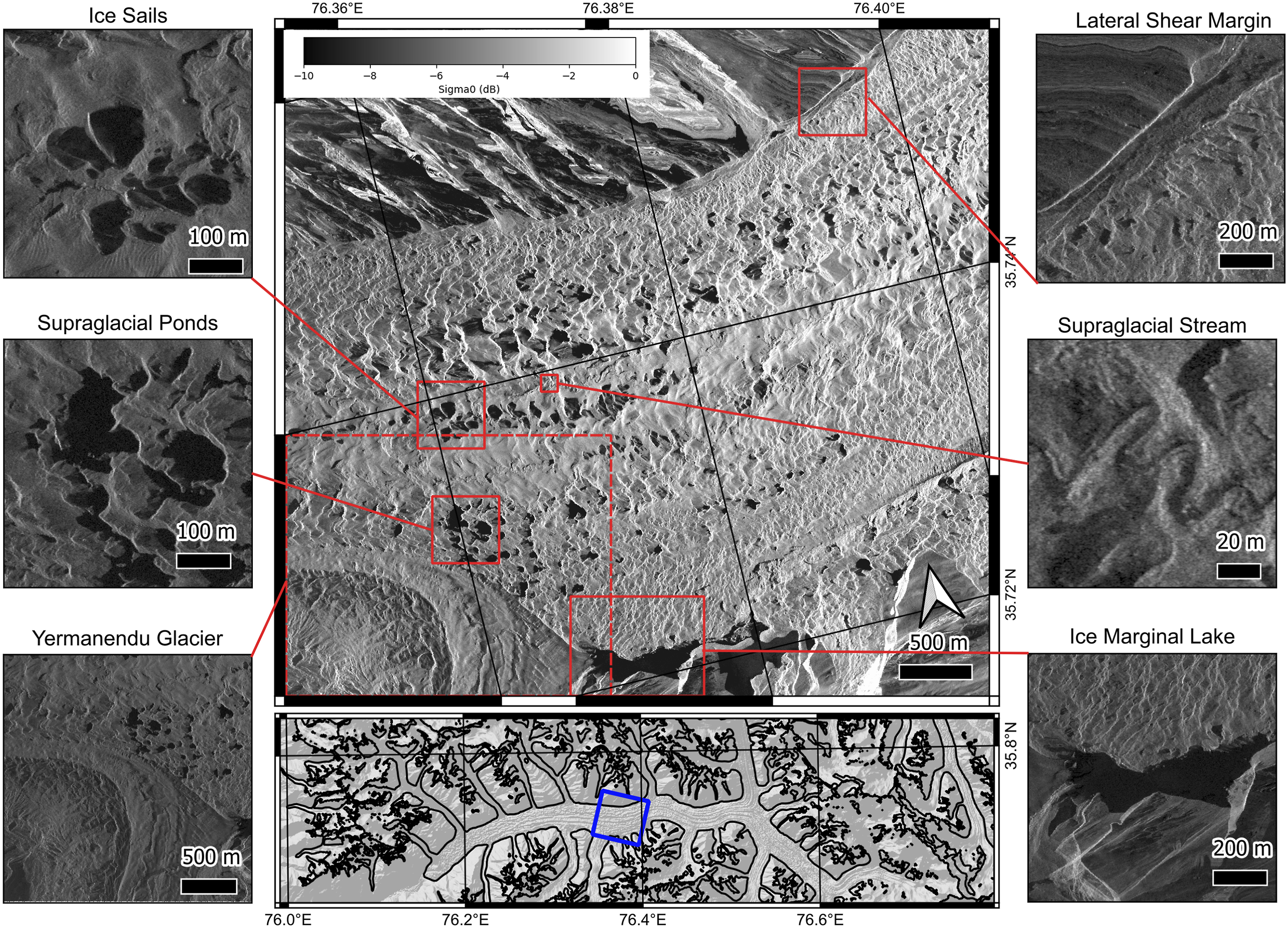

The climate around the Baltoro Glacier is characterized by cold, wet winters, mostly driven by westerly winds, and mild, dry summers. Summer precipitation is rare, although occasional intrusions of the Indian monsoon cause warm, wet spells (Farinotti et al., 2020). There is some evidence for an increase in Westerly driven precipitation in the Karakoram since 1979 from satellite and reanalysis data (Cannon et al., 2016) although some studies show no change (Palazzi et al., 2013), suggesting that the effect is minimal if present. As with precipitation, there is some evidence of recent summer cooling in the Karakoram (Hasson et al., 2017), although tree ring records suggest that the region has undergone warming in line with the rest of High Mountain Asia (Asad et al., 2017).

Unlike elsewhere in High Mountain Asia, Karakoram glaciers have, until recently, been observed to have balanced or even positive mass budgets (Farinotti et al., 2020; Hewitt, 2005). Some studies have attributed this anomaly to these climatic changes (Bashir et al., 2017), whereas others have invoked changes in irrigation practice as a primary control (de Kok et al., 2018). Most recent analyses suggest that this anomalous period of mass gain is now over, however, meaning glaciers like Baltoro Glacier may enter a phase of slow-down and surface lowering, as most debris-covered glaciers further east in the range have experienced over recent decades (Dehecq et al., 2019; Hugonnet et al., 2021).

Data sources and methods

We measure the ice flow velocity of Baltoro Glacier by applying feature tracking to images acquired by three different satellite SAR sensors (Table 1). The sensors have multiple imaging modes with different resolutions from which we select a mix of medium (5–20 m), fine (3 m), and very-fine (0.35 m) resolutions for our analyses. We focus primarily on a pair of Capella images acquired on July 15 and July 21 2021 with a difference in incidence angle of just 0.3° (Table 2).

Table 1.

Comparison of SAR satellites used in this project.

Satellite	Sentinel-1	TerraSAR-X	Capella
Operator	ESA	DLR	Capella Space
No. of satellites (as of April 2025)	2^a	2	10
First launch year	2014	2007	2018
Revisit time	12 days^a	11 days	<1 day^b
Centre frequency	5.405 GHz (C-band)	9.65 GHz (X-band)	9.65 GHz (X-band)
Imaging mode	Interferometric wide	Stripmap	Spotlight
Spatial resolution	5 × 20 m	3 m	0.35 m
Swath width	250 km	50 km	5 km
Noise equivalent sigma0	−30 dB to −23 dB	−19 dB	−14 dB to −10 dB
References	Geudtner et al. (2014)	Werninghaus and Buckreuss (2010)	Stringham et al. (2019)

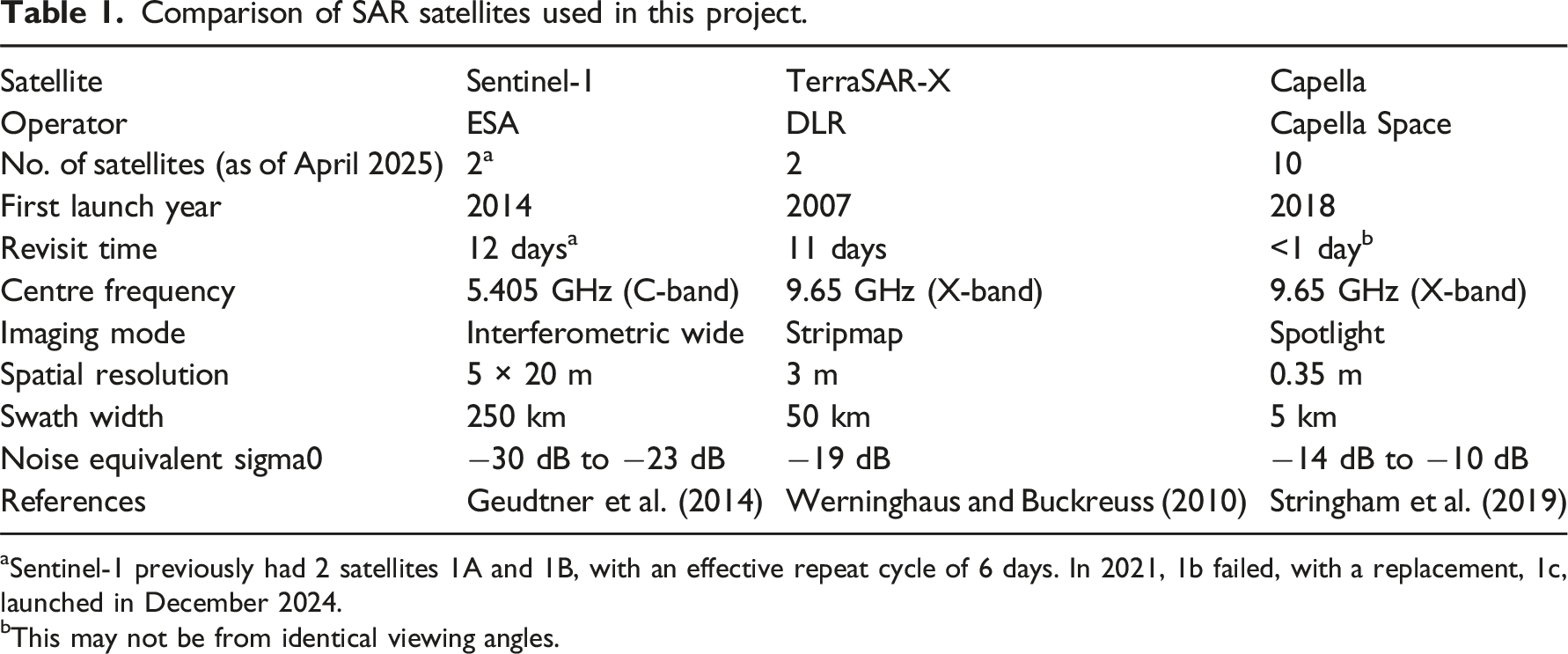
^aSentinel-1 previously had 2 satellites 1A and 1B, with an effective repeat cycle of 6 days. In 2021, 1b failed, with a replacement, 1c, launched in December 2024.

^bThis may not be from identical viewing angles.

Table 2.

Images used for feature tracking.

Satellite	Acquisition mode	Product	Pol	Date	Time	Inc. angle (°)	Orientation	δT (d)
Capella-3	Spotlight	GEC	HH	2021-07-15	05:02:06	26.8	Descending	8
Capella-3	Spotlight	GEC	HH	2021-07-23	05:02:10	27.1	Descending	8
TerraSAR-X	Stripmap	SSC^a	VV/VH	2016-05-24	01:02:59	33.7	Descending	44
TerraSAR-X	Stripmap	SSC	VV/VH	2016-07-07	01:03:00	33.7	Descending	44
Sentinel-1A	IW	SLC	HH	2021-07-02	12:57:15	43.2	Ascending	24
Sentinel-1A	IW	SLC	HH	2021-07-26	12:57:18	43.2	Ascending	24

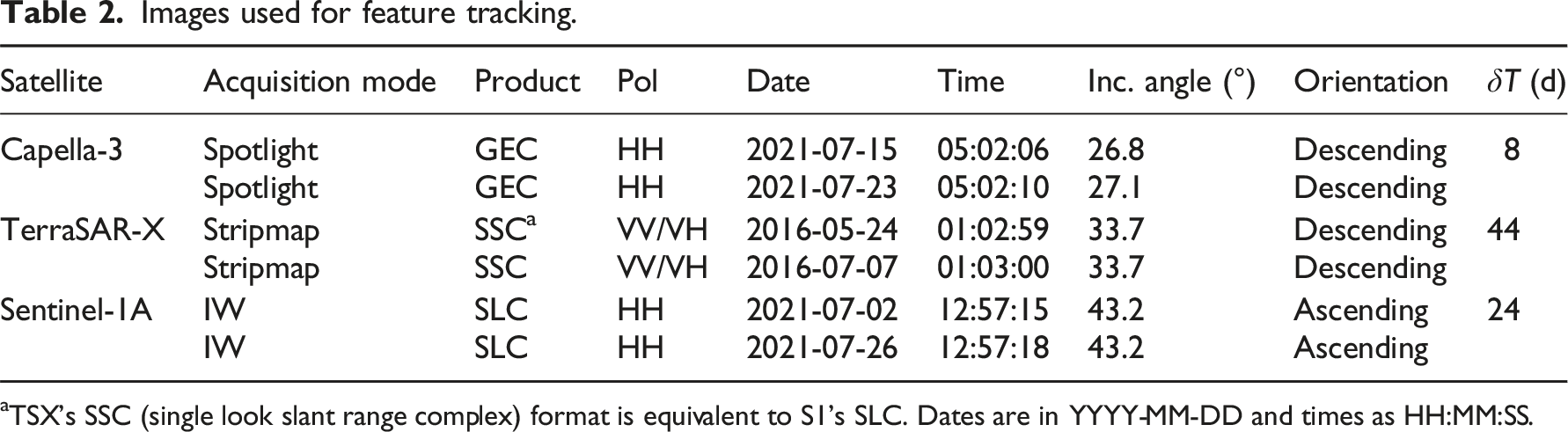
^aTSX’s SSC (single look slant range complex) format is equivalent to S1’s SLC. Dates are in YYYY-MM-DD and times as HH:MM:SS.

In addition to SAR imagery, we used the Copernicus GLO-30 m Digital Elevation Model (DEM) for processing and analysis. The Copernicus GLO-30 DEM is an amalgamation of data derived from the WorldDEM, supplemented with multiple other DEM sources. Consequently, errors are likely to vary spatially. Within the WorldDEM coverage, 64.7% of the land was found to be within 2 m of the more accurate ICESat altimeter data, and only 0.8% of the land exhibited a vertical difference of over 10 m (Airbus Defence and Space, 2022).

Feature tracking of SAR images is performed using cross-correlation of pixel intensities to identify distinct features on the surface between images in GAMMA (Werner et al., 2000). A moving window (also known as a chip or a patch) of a given size is moved across both images, with cross-correlation used to measure the similarity between the two windows. The location of peak cross-correlation is considered a match, and the offset between the two windows on the co-registered images is used to calculate the displacement (Luckman et al., 2007; Schubert et al., 2013). The size of the window is crucial, as for features to be tracked the chosen size needs to reflect both the size of distinct features on the ground (e.g. ponds and crevasses) and expected motion. As we track the motion of the entire window, the choice of window size influences the observed offsets (Huang and Li, 2011). For each satellite, we experiment with a range of window sizes in order to determine optimal patch sizes.

We experimented with a range of different window sizes (Supplemental Figure 1), but for our main analysis focused on comparing the results of feature tracking with 128 × 128 pixel windows for Capella and TSX, and 128 × 512 for S1, which provides a good balance between detail, noise, and computational time. In ground metres, this means each window covers 44.8 m within a Capella image, 384 m for TSX and 2560 m for S1, and we thus track features on a variety of scales. We use a step size of one pixel, which means that each window is one pixel over from the previous window. This allows us to achieve the highest possible resolution ice flow map albeit at the cost of computational time.

Each pair of images must be co-registered to ensure that the measured offsets represent true ground motion. For S1 and TSX imagery, we co-registered the images in slant range and converted to ground range after the feature tracking algorithm in order to maximize the information available for the tracking algorithm. However, for our Capella pair, the small difference in incidence angle between the two images, uncertain footprint, and lack of stable ground within the scene prevented us from using SLC images. Instead, we chose to use the geocoded but non-terrain corrected product to avoid any distortions introduced by the orthorectification process, and these scenes were provided already co-registered to within a few pixels, which we were able to refine as part of our sub-pixel tracking approach.

Uncertainties in the final outputs differ between the sensors. In the specific case of Capella, difficulties in co-registering the image pair caused additional offsets to be detected by feature tracking which are not the result of true surface motion. In the case of S1 and TSX there is a small amount of additional error introduced during the ground-range conversion as a consequence of errors in the Copernicus GLO-30 DEM, as well as mismatches in the DEM resolution and the image resolution. DEM errors are unlikely to significantly affect the feature tracking, as the glacier surfaces of interest generally have low slope gradients (less than 5°), where DEM accuracy is at its maximum. Exceptions could be steep icefalls, and sections of glaciers with numerous crevasses or supraglacial ponds. Another potential source of error arises from changes that may have occurred between the acquisition of the DEM and the imagery. The Copernicus GLO-30 DEM was derived from imagery obtained between 2011 and 2015, while our SAR imagery was collected between 2014 and 2021. Changes may take the form of thinning, most of which will be well below 1 m per year (Maurer et al., 2019). As long as the thinning rate is mostly uniform across the glacier surface, this is unlikely to cause significant error in the velocity measurements. Shifting surface features such as supraglacial ponds and crevasses may introduce small, localized errors, although these are unlikely to be significant. We filter our final offsets to retain only those with a cross-correlation peak >0.2 (0–1 scale, where 1 is perfect cross-correlation), thus removing the majority of low-confidence data.

It is not possible to robustly quantify these sensor-specific uncertainties, but we directly address those relating to co-registration of the Capella imagery in our evaluation of the feature tracking outputs below. Uncertainty due to sensor resolution is estimated at around 1/10th of a pixel (Friedl et al., 2021), divided by the temporal baseline. This equates to 0.004 m/day for the 8-day Capella pair, 0.006 m/day for the 44-day TSX pair, and 0.084 m/day for the 24-day S1 pair. The level of noise, caused partly by on-board satellite electronics, also varies between sensors and may introduce additional uncertainty to feature tracking by introducing random change between images. Additionally, there may be differences in measured velocity which are caused by temporal variations in ice flow. In the case of Capella and S1, this is likely to be negligible as both pairs were captured during the same period in July 2021. The TSX pair was captured in 2016; however, ITS_LIVE data do not show significant differences in velocity between these time periods (Gardner et al., 2019). The absolute velocities of each image source are also of secondary importance since we are primarily interested in the level of detail afforded by the Capella imagery, and its ability to shed light on local scale variabilities in flow.

In the absence of ground truth velocity measurements, we utilize the GLAcier Feature Tracking Testkit (GLAFT) (Zheng et al., 2023) to assess the distribution of measured velocity values in both the x (horizontal) and y (vertical) directions. Initially, the tool is applied over stable ground, where no movement is expected, in order to evaluate the performance of the measurements. The width of the resulting spread of velocity values serves as an indicator of measurement uncertainty, with a wider spread corresponding to greater uncertainty. Additionally, if the centre of the spread deviates from the origin (0, 0), this suggests the presence of a systematic bias. Secondly, we use GLAFT to analyse the strain field across the flowing regions of our image. Since the true glacier velocity field is expected to exhibit spatial coherence, high spatial variability in strain rates may suggest errors in the feature-tracking process, potentially reflecting mismatches or noise rather than natural glacier dynamics. Conversely, very low strain variability might indicate that important flow details have been lost.

Results

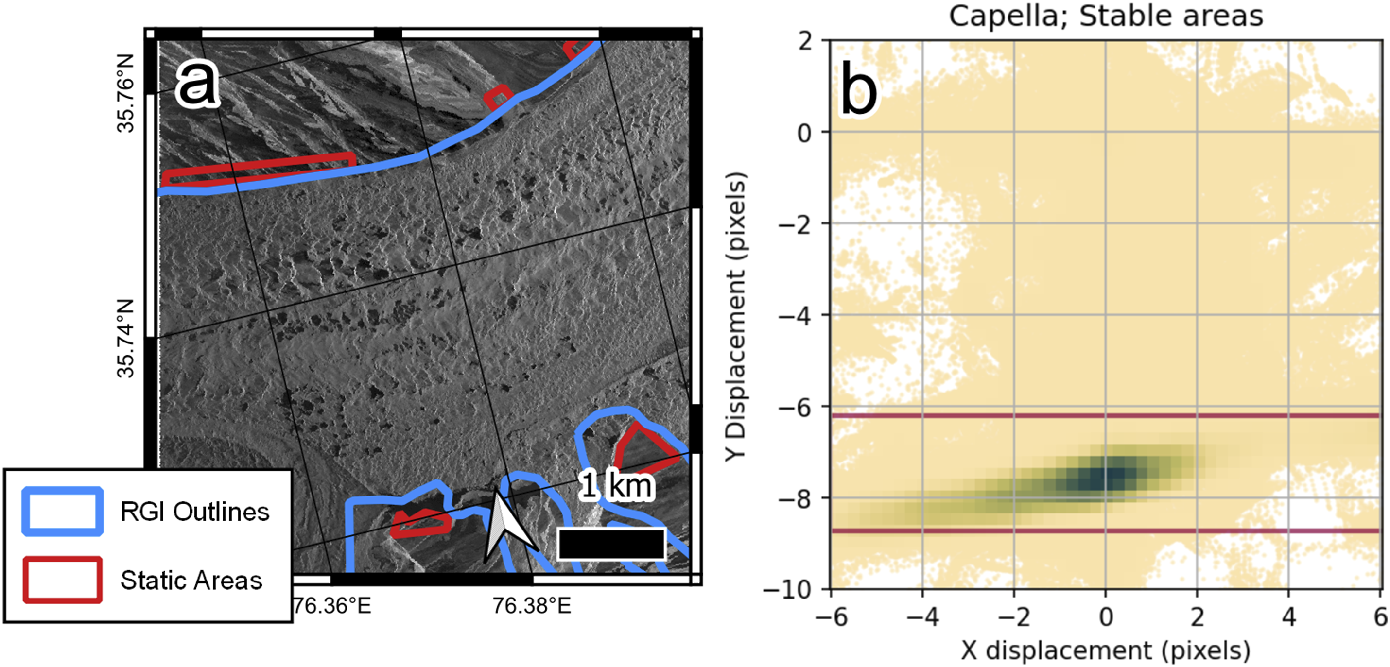
Feature tracking of the raw geocoded Capella product yielded a coherent and comprehensive velocity field across the glacier surface (Figure 3, left panels). However, interrogation of the values from areas of stable ground using GLAFT (Zheng et al., 2023) indicated relatively high errors (Figure 4). We quantified these displacements by sampling five areas of relatively flat, stable ground located on the margins of the glacier. These areas of stable ground were initially derived from RGI outlines and then manually corrected to ensure that they do not overlap with unstable areas. These erroneous displacements cannot be attributed to any natural process such as debris flow or landslides, as there is no evidence of such events from optical imagery during our observation period. We assumed that since the elevation and relief of these stable areas closely reflect those of the glacier surface, the erroneous displacements measured could also be considered consistent between the two.

Figure 3.

Velocity maps before and after applying the correction. (a) and (b) show the magnitude of the velocity, (c) and (d) show the x (azimuth) component of velocity, (e) and (f) show the y (range) component of velocity.

Figure 4.

Process used to quantify the co-registration error between our Capella image pair. (a) Shows the Capella SAR image from 15 July 2021 with the glacier boundaries from the Randolph Glacier Inventory (RGI) and the static areas chosen in red. Note the lack of flat, ice-free ground within the image frame and the errors in the RGI outlines. (b) Shows the observed x and y displacements of each offset measurement within the static areas, with the areas of high kernel density estimate (KDE) highlighted in green. The red box covers the area where the KDE is within the maximum density. Stable areas (b) plotted using GLAFT (Zheng et al., 2023).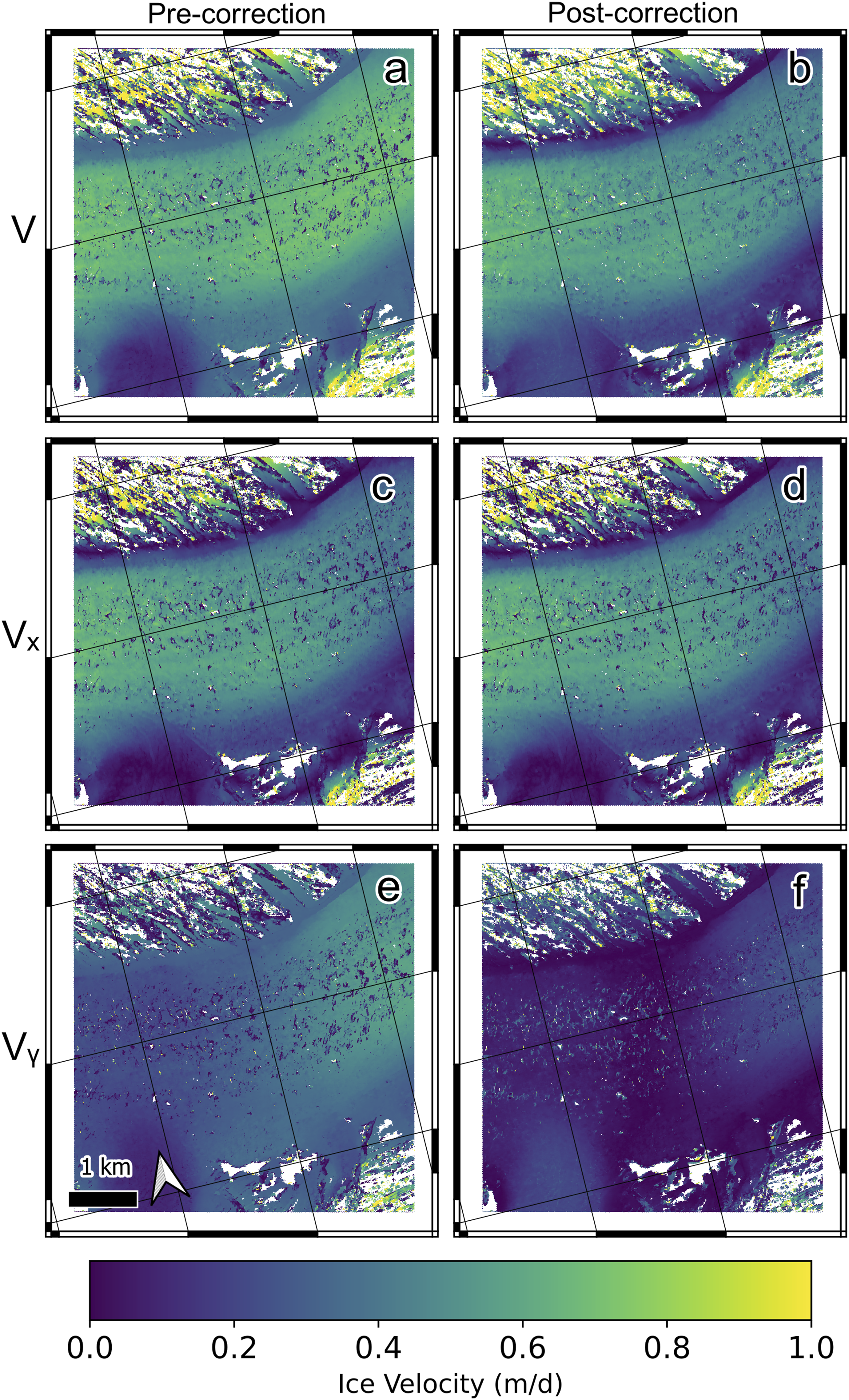

While there is noticeable variability in measured offsets in stable areas, the majority of observations centre around displacements of x = 0 and y = −7. Guided by these findings, we applied a uniform shift in y of 7 pixels. Figure 3 (right panels) shows the impact of this correction, with the principal outcome being an overall reduction in the measured velocities (equating to approximately 0.2 m/day along the glacier centreline).

The corrected data show that ice flow at the margins is close to zero, although significant erroneous displacements remain visible higher on the ice-free slopes. The correction improved the depiction of the Yermanendu Glacier’s confluence with the Baltoro Glacier (in the lower left part of the image). In the uncorrected version, the Yermanendu Glacier appeared motionless, as its velocity (dominated by the Y component) was negated by the co-registration error. Following the correction, the glacier flow is clearly visible, gradually moving northwards and deviating westward as it feeds into the Baltoro Glacier.

Nevertheless, measured displacements in the corrected datasets, derived from stable ground, suggest that even post-correction the Capella-derived velocity data contain greater uncertainty than those derived from S1 and TSX, with a notable spread of values of the order of 0.1 m/day (Figure 5). Offsets derived from TSX and S1 show an order of magnitude less variability over stable ground (0.01 m/day for TSX and 0.03 m/day for S1). Observed strain appears to be clustered around zero for all three sensors, with variability increasing with the resolution of the sensor.

Figure 5.

Observed x and y components of velocity over stable ground (a), (b), and (c), and distribution of normal and shear strain rates (d), (e), and (f) across the flowing area of Baltoro covered by the Capella image. The red box covers the area where the KDE is within 1/ⅇ^(z^2/2) of maximum density. δx, δy, δx′x′, and δx′y′ are half-width of the boxes and serve as a measure of the performance. Plotted using GLAFT (Zheng et al., 2023).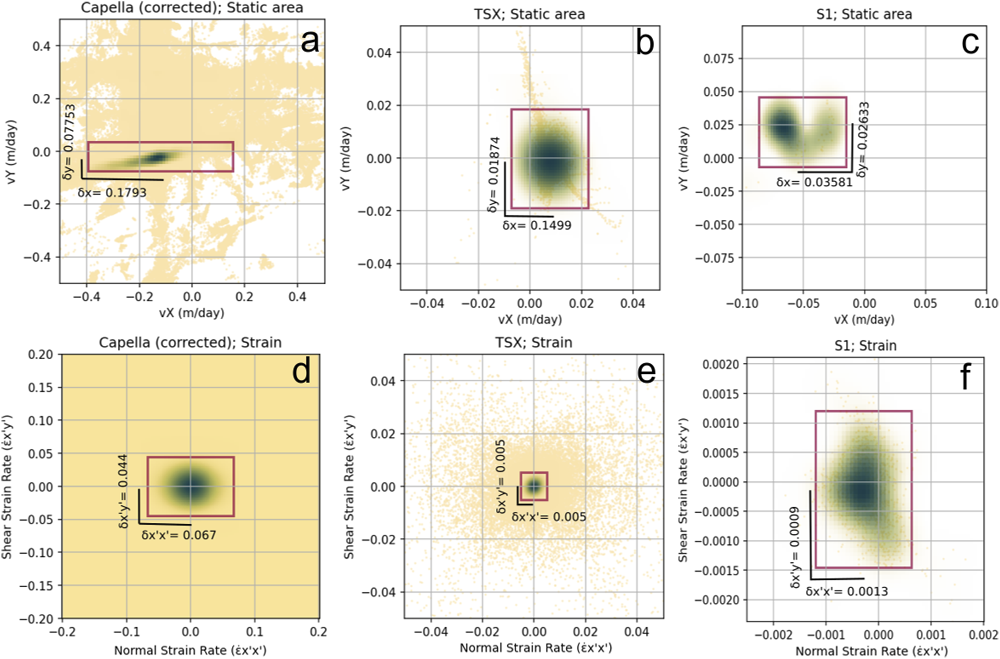

Velocity data generated from very-fine resolution Capella Spotlight imagery is visibly very detailed but only covers a small area of Baltoro Glacier (25 km²) (Figure 6). The flow pattern created by the intersection with the Yermanendu Glacier is resolved in fine detail within the Capella data and is also evident within the TSX velocities, but it is only very subtly depicted within the S1 output. The along-flow profiles (Figure 7, transect A) show some differences in measured velocities between sensors. The Capella-derived values match those derived from S1 in the across-flow profiles (Figure 7, transects B, C, and D), as well as in the last 2.5 km of the along-flow profile, but show a difference of 0.2 m/day compared to TSX and S1 in the first 500 m of the along-flow profile. S1-derived velocities are noticeably lower than TSX- and Capella-derived velocities in the first 2.5 km of the along-flow profile, as well as in the centre of the glacier, as shown in two of the across-flow profiles (Figure 7, transects B and C). It is worth noting that the along-flow transect crosses mainly a unit of dark debris with multiple ice sails (Evatt et al., 2017). It is likely that these ice sails undergo significant surface ablation between our two Capella Space images, which results in temporal incoherence and inability to feature track. It is also possible that the relief of these features impacts the velocity measurements.

Figure 6.

Comparison of velocity maps created using the three sensors and imaging modes, illustrating differences in footprint sizes and variability in the detail produced from each input dataset.

Figure 7.

Surface velocity data for the Baltoro area covered by Capella images, obtained from feature tracking of (a) Capella, (b) Sentinel-1, and (c) TerraSAR-X data. The window sizes shown here are 128 × 128 for Capella and TSX and 128 × 512 for Sentinel-1. Comparative plots along transects A (along flow) and B, C, and D (across flow) are presented below.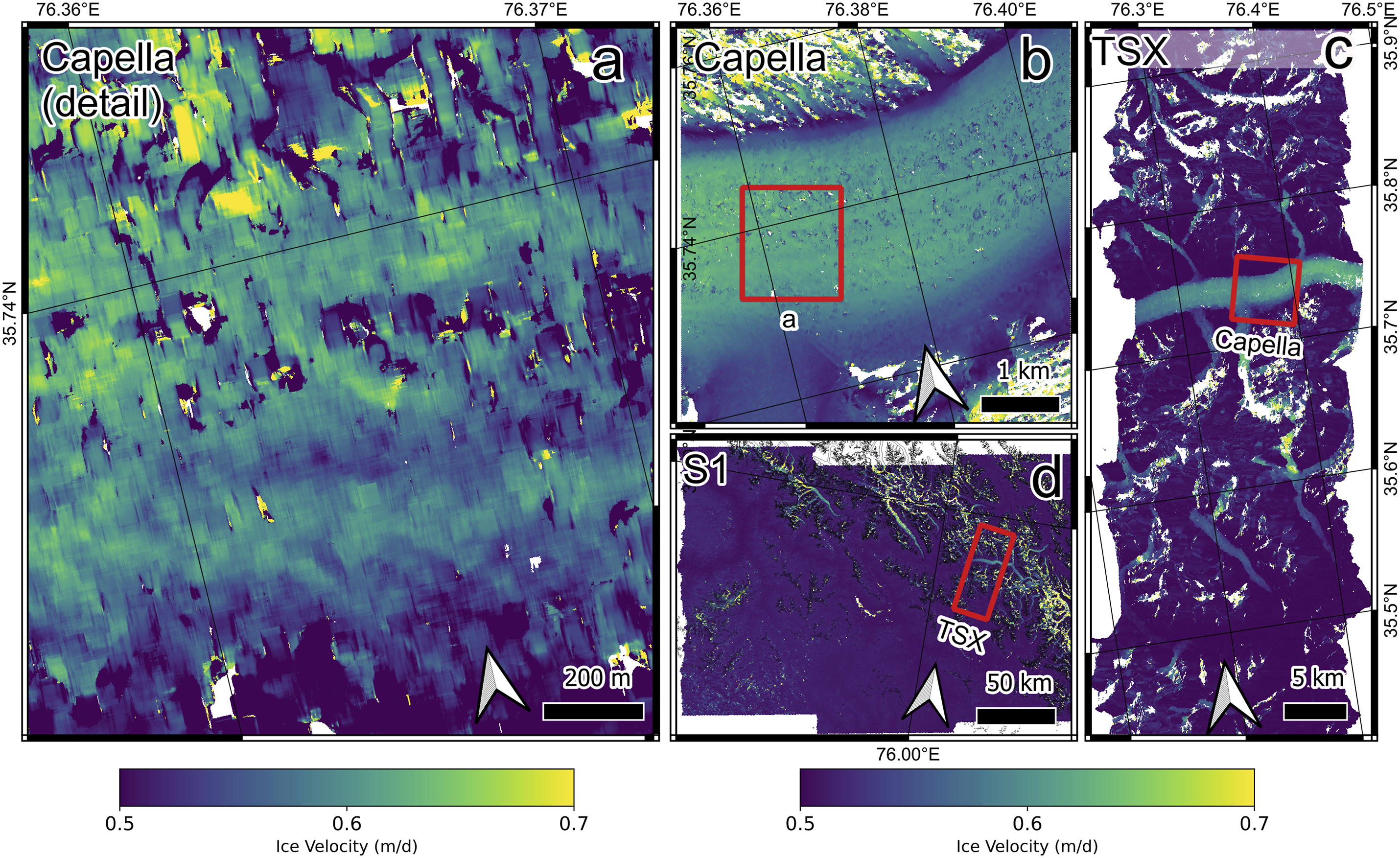

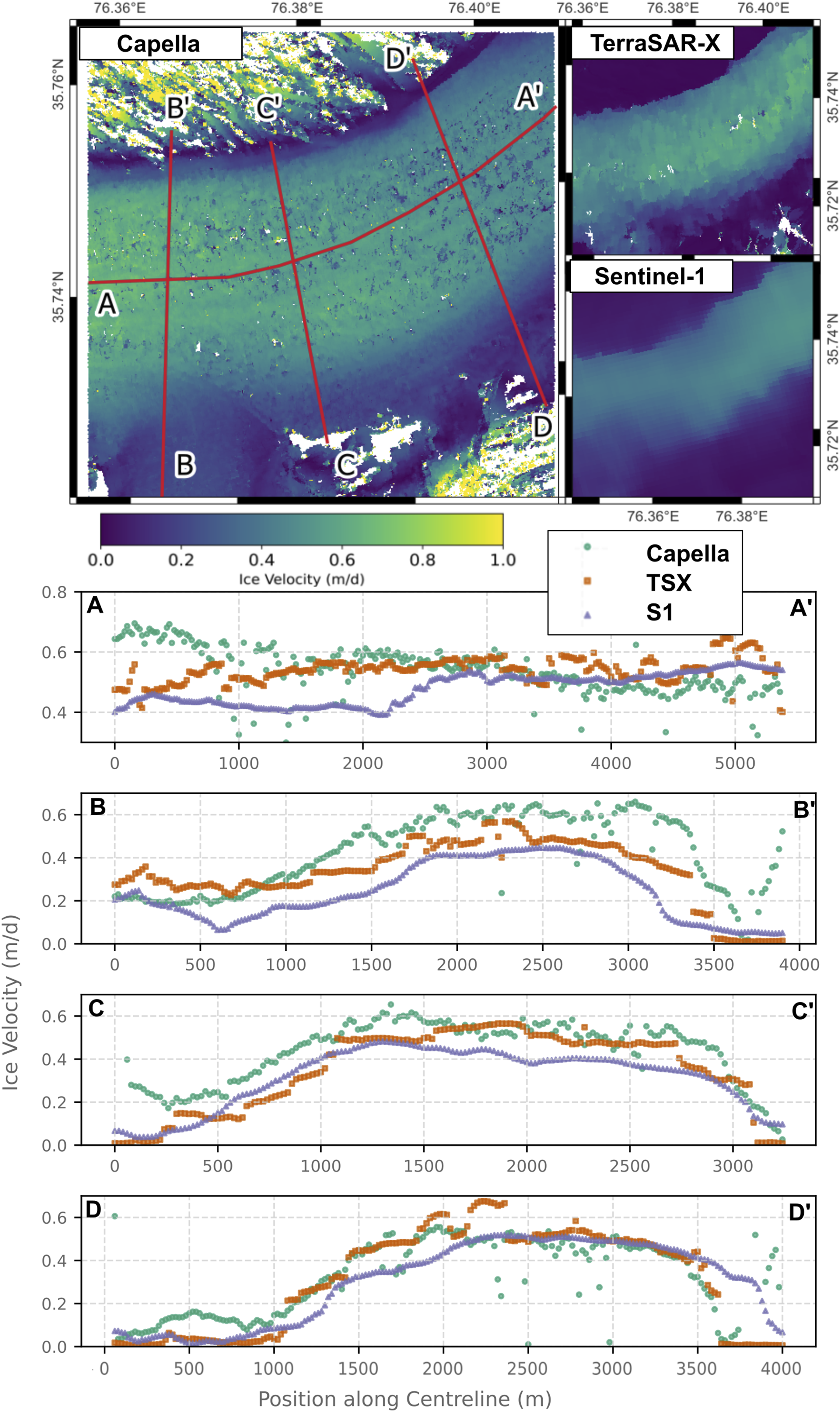
All three outputs show across-flow velocities with a concave shape, with faster velocities in the centre of the glacier and slower flow near to the margins (Figure 7, transects B, C, and D). On the southern shear margin (Figure 7, transects C and D), all sensors capture the gradual slowdown of ice flow from over 1 km from the margin. On the northern margin, Capella- and TSX-derived velocities show a sudden drop-off within 100 m of the shear margin. On the other hand, Sentinel-1 data show a more gradual deceleration towards the margin.

The Capella-derived velocities display fine-scale spatial variations in ice flow (Figure 8). In particular, a steep reduction in velocity is evident near to the glacier margin (a), as well as at the confluence between Baltoro Glacier and Yermanendu Glacier (c). We also detect subtle but smooth variations in surface velocity (<0.05 m/day) on a relatively featureless part of the glacier (f). Also visible in Figure 5(a), these coherent variations of observed ice flow velocity appear to follow the undulating topography of the glacier surface, parallel to the direction of ice flow. Other observed fine-scale variations are due to errors and noise in feature tracking with a small window size. We note small gaps in measurements above a supraglacial pond (b) and a supraglacial stream (e), the latter of which appears to be surrounded by wet snow. There are clear fine-scale velocity differences in areas of extreme surface relief, such as at an ice cliff (d), which are likely caused by the difference in viewing angle.

Figure 8.

Ice velocity transects, derived from Capella imagery, overlain on Capella SAR image from 15 July 2021. Panels on left show six different surface features and the observed spatial variability of ice flow.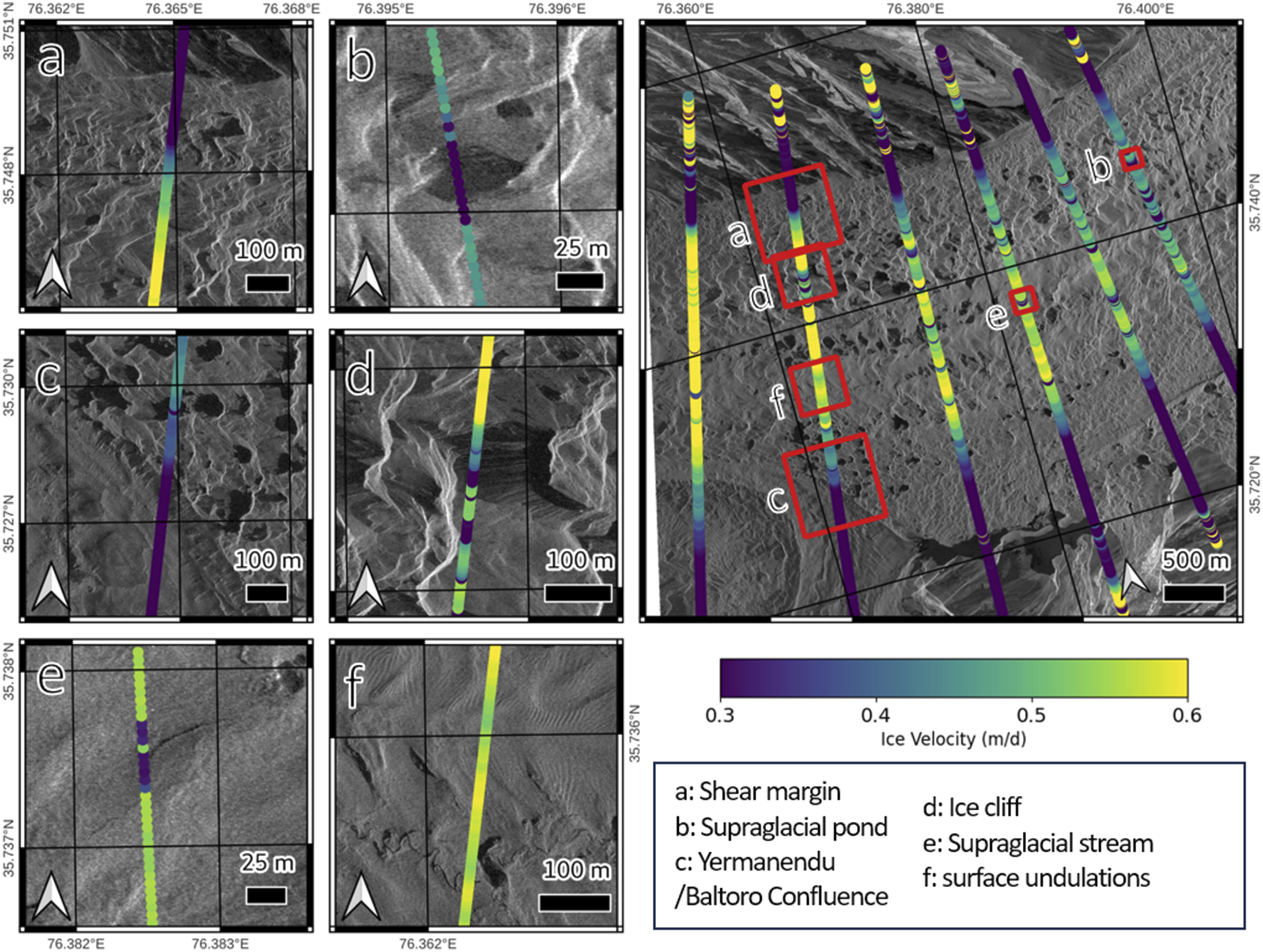

In our experiments with various window sizes (Supplemental Figure 1) we identified a tradeoff between sharpness and uncertainty, with small window sizes (16–64 pixels) producing sharp but noisy outputs and larger window sizes (128–512 pixels) resulting in smoother outputs with less gaps, but at the cost of longer computational time. The optimal window size for tracking Capella imagery (128 × 128 (44.8 m)) appears to be approximately twice that for and Sentinel-1 (128 × 128 (2560 m)).

Discussion

Our results demonstrate that feature tracking with very-fine resolution SAR imagery, such as that acquired by Capella satellites, can reveal fine-scale variations in ice flow both parallel and perpendicular to flow. Detailed analysis of the velocity fields (Figure 8) reveals that some of these observed variations result from the tracking window being smaller than incoherent features such as supraglacial ponds or streams. However, this enhanced resolution, when compared to more commonly used image data sources, reveals ice flow variability that is likely real.

In particular, we observe a distinct ≈100 m wide zone at the northern margin of the glacier (Figure 8(a)), in which ice flow decreases sharply from over to 0.3 m/day down to 0 m/day. In this zone, resistive stresses are high owing to the friction between the valley wall and the glacier ice, impacting the broader glacier flow field. The dynamics and rheology of glacier shear margins, and their impact on ice flow, are relatively poorly understood given that they are rarely resolved in satellite observations and are often difficult to access in the field. Fine-resolution velocity data like those derived from Capella therefore enable us to derive new information about rheological mechanisms operating at glacier margins and, coupled with in situ measurements of ice temperature (Miles et al., 2018), could further our understanding of the relationship between glacier thermal regime, glacier flow, and erosion. In particular, sediment quarrying and abrasion depend on the rheology of the ice, and sediment entrainment can be enhanced within this zone (Alley et al., 2019). Additional observations from other sites, and throughout the melt season, therefore have the potential to shed additional light on key landscape-shaping processes, as well as providing more refined validation and calibration products for glacier modelling experiments (e.g. Rowan et al., 2021).

The clearly defined flow characteristics of the Yermanendu Glacier show that fine-resolution velocity data offer the possibility to include the ice dynamics of small glaciers, within relevant inventories. In the Karakoram specifically, many small glaciers are known from field observations to be surge-type (though not Yermanendu Glacier) but are often missing from (or are poorly characterized in) records of surge events which are largely derived from coarse, broad-scale velocity measurements (Bhambri et al., 2017). Detailed observations of surge events on smaller, high-altitude glaciers would add to growing literature on their evolutionary characteristics (Quincey et al., 2015) as well as to inform frameworks for understanding surge behaviour and control (Benn et al., 2023).

Lateral fluctuations in ice velocity (<0.05 m/day), manifesting as wave-like undulations traversing the glacier’s width, can be discerned in Figure 6(a) and, to a lesser extent, in Figure 8(f). These velocity variations seemingly correlate with topographic features, displaying faster velocities within a trough serving as a conduit for a supraglacial stream and within a section accommodating numerous supraglacial ponds. The mechanisms driving these variations are unclear, but they could be attributed to undulations in sub-glacial topography, or may even reflect the locations of subglacial channels where friction is minimized. Indeed, detailed flow fields such as these hold potential for highlighting local differences in subglacial friction that translate to small variations in surface ice velocity, such as the presence of seasonal sticky spots which are otherwise only detectable using in situ means (Willis et al., 2003). Additional research is needed to corroborate the occurrence of such variability across disparate regions of the glacier and throughout varying seasonal conditions.

We also observed small (up to 0.2 m/day) but significant differences in velocity between the three sensors. The differences between TSX and Capella/S1 are likely caused by real variations in ice velocity between the timings of image acquisition (May–July 2016 for TSX and July 2021 for S1/Capella). The magnitude of these differences is well within the range of seasonal variability observed at this location (>0.3 m/day) (Quincey et al., 2009; Wendleder et al., 2018) and consistent with the expectation that velocities are higher earlier in the summer when the drainage system is still inefficient. Substantial differences between Sentinel-1 and Capella-derived velocities are only observed in the upper portion of our data, with differences of up to 0.2 m/day. While we cannot at present exclude the possibility of this being an artefact of the correction procedure, it is feasible that these data capture a slow-down in ice velocity in the upper part of the glacier as the melt season progresses.

While in situ derived ground truth measurements or higher-resolution sensors would ideally serve as validation benchmarks, S1 and TSX nonetheless provide valuable validation datasets. First, both TSX and S1 have a long history of use for ice velocity measurements (e.g. Guo et al., 2020; Lemos et al., 2018; Neelmeijer et al., 2014). We therefore have well-developed understanding of the typical uncertainty and sources of error associated with these sensors (discussed in papers cited above) and with this method (Strozzi et al., 2002) and they have been shown to perform well over texture-rich and low-angled surfaces like debris-covered glaciers (Gu et al., 2024). Second, while the spatial resolution of S1/TSX may be lower than that of Capella, factors such as consistency of viewing angle and geocoding accuracy are both superior and better understood. This provides an internally consistent system for deriving velocity measurements that Capella cannot currently match, and an independent and robust measure with which to validate our data, albeit at reduced spatial resolution.

Despite the promise shown within these results, there are considerable challenges to overcome before the processing of velocity fields from Capella imagery may become routine. Most significantly, the co-registration of images required an innovative, and probably imperfect, solution. The co-registration of very high resolution imagery has been a known challenge in optical imagery since the launch of QuickBird in 2001 (Arévalo and González, 2008), and solutions typically involve the use of ground control points located on flat, stable ground (Guo et al., 2022), which our images lacked. While our flat, linear correction for this issue significantly improved the results, differences remain between the Capella and Sentinel-1/TerraSAR-X datasets. This suggests that the ‘flat’ correction we applied, based on motion over stable ground, may not capture the spatially varying distortion within the image owing to local scale relief. A more complex correction could potentially be applied with a better understanding of the geometric differences between image acquisitions and the broader landscape topography. In areas where high-resolution DEMs are available (e.g. High Mountain Asia 8 m DMA (Shean, 2017)), these may be used to remove geometric distortions. Previous studies have used LIDAR-derived DEMs to co-register geometrically inconsistent very-fine resolution imagery (Teo and Huang, 2013), although this would be difficult to implement at Baltoro where overflights and drone surveys are largely prohibited with it being so close to a militarized zone. Alternatively, co-registration methods based on spectral diversity rather than cross-correlation could be explored (Scheiber and Moreira, 2000).

The need for such a correction could be eliminated entirely by ensuring acquisitions contain sufficient flat, stable ground to aid co-registration. In practice, this is applicable only to smaller glaciers whose width fits within the spotlight frame of 5 × 5 km. Alternatively, other Capella-derived imaging modes, which have larger footprints but coarser resolutions, could offer a solution where such fine resolution is not required. For example, the sliding spotlight mode has a footprint of 5 × 10 km and a resolution of up to 0.8 m, while the Stripmap mode has a footprint of 5 × 20 km and a resolution of up to 1.2 m. Improved control of orbital parameters to create more consistent viewing angles and footprints between revisits would also greatly reduce the need for such corrections, although the small size and low fuel supply of satellites such as Capella may render this difficult. Finer-resolution DEMs than those that currently exist would help to correct for topographic geometric distortions in the SAR image. At present, the inventory of consecutive very-fine resolution SAR images of mountain glaciers suitable for feature tracking is insufficient to assess whether co-registration will be a recurrent issue.

The benefits of using very-fine resolution SAR data such as Capella are clear, but whether they outweigh the uncertainties described above is largely dependent on the specific application. For analyses that require glacier-wide flow fields (e.g. studies of specific mass balance (Miles et al., 2021)) or where the ice is very fast-flowing and/or incoherent (e.g. during surge events (Paul et al., 2021)), the long Sentinel satellite record provides an adequate means of deriving high-quality velocity data that is well constrained in terms of error and without great computational expense. The sub-metre resolution of Capella shows greatest promise for detailed investigations of ice-flow processes and their spatial variability at a very local scale. Based on our analyses, we see potential for the long-term integration of fine-resolution images for velocity analyses in the following key areas.

Near-stagnant glacier tongues

In many regions, such as the Himalaya, mass loss is the main driver of glacier slowdown (Dehecq et al., 2019). Glaciers are frequently characterized as being stagnant once their velocities are too low to be resolved using coarse resolution imagery. Yet few glaciers are truly stagnant, with ice deformation persisting under gravitational forces, albeit at very low rates. There is GPS evidence from Khumbu Glacier’s reportedly inactive tongue of motion in the order of 1–3 ma (0.003–0.009 m/d), driven solely by ice deformation (Watson et al., 2017). At this velocity, only 19–58 days are needed for an object to travel through half Capella pixel (0.35 m), which indicates that fine-resolution imagery could be used to detect motion of near-stagnant ice, such that it can be more robustly represented in dynamic models of ice evolution.

Short-term ice flow variations

The seasonal variability of mountain glaciers remains poorly understood, and velocity time series of sufficient temporal resolution to observe seasonal variability remain scarce. While Sentinel-1 is capable of observing seasonal variability of large glaciers such as Baltoro, the quality of measurements on smaller glaciers (such as Yermanendu in our scene) is poor. Larger glaciers tend to be thicker, and therefore able to support a basal hydrology and seasonality, whereas small glaciers are often not but may still exhibit pockets of warm ice that respond to temperature rises during the summer season. Fine-resolution sensors therefore open up the possibility of studying seasonal velocity signals in glaciers that are hitherto largely ignored in studies of ice dynamics. The short repeat capability of such satellite swarms also allows us to observe sub-seasonal ice flow variability. Prior to the loss of Sentinel-1B, a temporal resolution of 6 days was the finest available, meaning analyses of short-term variations in flow, such as in response to a pond drainage event, were not possible, as they were smoothed out over the longer observation window. The additional benefit of fine spatial resolution also means that displacements over such short timescales can now be robustly quantified, whereas they were rarely large enough to be detected in Sentinel image pairs even over the shortest temporal window. This could offer potential for better characterizing spring events, for example, and the response of mountain glaciers to sudden onset melt events, or heavy periods of precipitation, or drainages of supraglacial lakes (Nanni et al., 2023; Stevens et al., 2022; Wendleder et al., 2023).

Rock glaciers

Rock glaciers exist on a continuum between debris-covered glaciers and groups of clasts interwoven with ice (Anderson et al., 2018), and they may form from receding, stagnant glacier tongues (Jones et al., 2019). Rock glaciers flow slowly as ice deforms under the influence of gravity. Few measurements of rock glacier velocity exist, as their slow flows are typically based on in situ measurements, either from GPS (Cicoira et al., 2019; Kellerer-Pirklbauer et al., 2018), or from uncrewed aerial vehicle (UAV) imagery (Groh and Blöthe, 2019), all of which identify spatial and seasonal ice flow variability. Rock glacier velocities have been measured using InSAR and offset tracking of Sentinel-1, as well as fine-resolution TerraSAR-X and Cosmo-SkyMed (1–2 m pixel size) images (Strozzi et al., 2020), although this resolution was still too coarse to resolve fine spatial and temporal flow differences. However, sub-metre resolution satellite imagery may be sufficient to detect subtle variations in rock glacier flow and identify active or inactive parts of rock glacier without the need to employ in situ methods.

Glacier collapses

Glacier collapse events are increasingly impacting mountainous regions as they warm and become more unstable. The velocity of the Aru Glaciers, Tibet, which collapsed in 2016, accelerated in the years prior to the event, and crevasses appeared on the glacier surface during the final few months (Gilbert et al., 2018; Tian et al., 2017). The small footprint of very-fine resolution imagery such as Capella spotlight products currently makes it impractical to identify at-risk glaciers, such as the Aru Glaciers, over large areas, but they could theoretically be deployed to monitor areas of specific concern to detect substantial changes in ice dynamics. Similarly, they could provide early detection of glacier surge events by detecting accelerations in flow that are too subtle for more commonly applied coarser resolution sensors.

Conclusions

We have demonstrated here that feature tracking can be applied to sub-metre resolution SAR images to generate ice velocity data. These data reveal fine details that are not clearly visible with coarser resolution, such as the behaviour of distinct flow units within glaciers, the effect of the shear margins on ice flow, and slight (<0.05 m/d) variations in ice flow across the width of the glacier, coinciding with glacier surface topography. These small-scale features are not clearly visible from the coarser resolutions of TerraSAR-X and Sentinel-1 and demonstrate the potential of sub-metre SAR imagery to study glacier dynamics on a much finer scale than previously possible.

However, feature tracking very-fine resolution imagery also presents challenges, as the small footprint of Capella’s spotlight mode (5 × 5 km) does not cover large glaciers and restricts practical use cases to studies looking at either a small section of a larger glacier or to small glaciers. This issue can largely be overcome by adopting a combined approach with coarser resolution sensors which cover wider areas, such as Sentinel-1, and targeting the use of very-fine resolution images to limited areas of significant scientific, economic, or humanitarian interest.

Additionally, the slight difference in incidence angle combined with uncertainties in the geographic extent of the images makes co-registration very challenging. Ordinarily, this problem could be overcome by using ground control points located on flat, stable ground, but such areas are rarely found within the glacial environment. We were able to significantly reduce these co-registration errors by applying a flat correction to all offsets in the scene. However, residual differences between the Capella-derived ice flow maps and those derived from S1 and TSX suggest that this correction is not perfect.

The potential for very-fine resolution SAR imagery to be integrated into contemporary inventories characterizing glacier flow, as well as for quantifying the dynamics of small, slow-moving, seasonally variable, and possibly hazardous mountain glaciers, is therefore high in the long-term, but the consistency of imaging geometries between acquisitions requires improvement before these types of analysis can be operationalized at broad scale.

Supplemental Material

Supplemental Material - Feature tracking of sub-metre resolution Capella SAR imagery to measure mountain glacier ice flow

Supplemental Material for Feature tracking of sub-metre resolution Capella SAR imagery to measure mountain glacier ice flow by Jamie Izzard, Duncan J Quincey, John R Elliott, and Anna Wendleder in Journal of Progress in Physical Geography: Earth and Environment.

Footnotes

Acknowledgements

The authors acknowledge the use of TerraSAR-X data (©DLR, 2017), Sentinel-1 data, and Capella data (obtained from ).

Author contributions

Jamie Izzard: Conceptualization, methodology, software, formal analysis, investigation, data curation, writing – original draft, and visualization. Duncan J. Quincey: Conceptualization, methodology, writing – review and editing, supervision, and funding acquisition. John R. Elliott: Conceptualization, methodology, writing – review and editing, and supervision. Anna Wendleder: Resources, data curation, and writing – review and editing.

Declaration of conflicting interests

The author(s) declared no potential conflicts of interest with respect to the research, authorship, and/or publication of this article.

Funding

The author(s) disclosed receipt of the following financial support for the research, authorship, and/or publication of this article: This research has been supported by the Natural Environment Research Council (NERC) through an SENSE CDT studentship (grant no. NE/T00939X/1). JE acknowledges support from the Royal Society through his University Research Fellowship (UF150282).

ORCID iD

Jamie Izzard

Data Availability Statement

Data will be made available upon request.*

Supplemental Material

Supplemental material for this article is available online.

References

Airbus Defence and Space (2022) Copernicus Digital Elevation Model (DEM) Product Handbook, Issue 5.0. Airbus Defence and Space.

Alley

Cuffey

Zoet

(2019) Glacial erosion: status and outlook. Annals of Glaciology 60: 1–13. DOI: 10.1017/aog.2019.38.

Anderson

Armstrong

, et al. (2018) Glaciation of alpine valleys: the glacier – debris-covered glacier – rock glacier continuum. Geomorphology 311: 127–142. DOI: 10.1016/j.geomorph.2018.03.015.

Arévalo

González

(2008) An experimental evaluation of non-rigid registration techniques on quickbird satellite imagery. International Journal of Remote Sensing 29: 513–527. DOI: 10.1080/01431160701241910.

Asad

Zhu

Liang

, et al. (2017) Climate signal in tree-ring width chronologies of pinus wallichiana from the Karakoram mountains in northern Pakistan. Pakistan Journal of Botany 49(6): 2465-2473.

Azam

Kargel

Shea

, et al. (2021) Glaciohydrology of the himalaya-karakoram. Science 373: eabf3668. DOI: 10.1126/science.abf3668.

Bashir

Zeng

Gupta

, et al. (2017) A hydrometeorological perspective on the Karakoram anomaly using unique valley-based synoptic weather observations. Geophysical Research Letters 44(10): 470–478. DOI: 10.1002/2017GL075284.

Benn

Hewitt

Luckman

(2023) Enthalpy balance theory unifies diverse glacier surge behaviour. Annals of Glaciology 1–7: 88–94. DOI: 10.1017/aog.2023.23.

Bhambri

Hewitt

Kawishwar

, et al. (2017) Surge-type and surge-modified glaciers in the Karakoram. Scientific Reports 7: 15391. DOI: 10.1038/s41598-017-15473-8.

10.

Cannon

Carvalho

LMV

Jones

, et al. (2016) Winter westerly disturbance dynamics and precipitation in the western Himalaya and Karakoram: a wave-tracking approach. Theoretical and Applied Climatology 125: 27–44. DOI: 10.1007/s00704-015-1489-8.

11.

Cicoira

Beutel

Faillettaz

, et al. (2019) Water controls the seasonal rhythm of rock glacier flow. Earth and Planetary Science Letters 528: 115844. DOI: 10.1016/j.epsl.2019.115844.

12.

Copland

Pope

Bishop

, et al. (2009) Glacier velocities across the central Karakoram. Annals of Glaciology 50(52): 41–49. DOI: 10.3189/172756409789624229.

13.

de Kok

Tuinenburg

Bonekamp

PNJ

, et al. (2018) Irrigation as a potential driver for anomalous glacier behavior in High Mountain Asia. Geophysical Research Letters 45: 2047–2054. DOI: 10.1002/2017GL076158.

14.

Dehecq

Gourmelen

Gardner

, et al. (2019) Twenty-first century glacier slowdown driven by mass loss in High Mountain Asia. Nature Geoscience 12: 22–27. DOI: 10.1038/s41561-018-0271-9.

15.

Evatt

Mayer

Mallinson

, et al. (2017) The secret life of ice sails. Journal of Glaciology 63: 1049–1062. DOI: 10.1017/jog.2017.72.

16.

Farinotti

Immerzeel

de Kok

, et al. (2020) Manifestations and mechanisms of the Karakoram glacier anomaly. Nature Geoscience 13: 8–16. DOI: 10.1038/s41561-019-0513-5.

17.

Friedl

Seehaus

Braun

(2021) Global time series and temporal mosaics of glacier surface velocities derived from Sentinel-1 data. Earth System Science Data 13: 4653–4675. DOI: 10.5194/essd-13-4653-2021.

18.

Gardner

Fahnestock

Scambos

(2019) ITS_LIVE Regional Glacier and Ice Sheet Surface Velocities. Boulder, CO: NASA National Snow and Ice Data Center Distributed Active Archive Center.

19.

Geudtner

Torres

Snoeij

, et al. (2014) Sentinel-1 system capabilities and applications. In: 2014 IEEE geoscience and remote sensing symposium, Quebec City, QC, 13–18 July 2014, 1457–1460. IEEE. DOI: 10.1109/IGARSS.2014.6946711.

20.

Gibson

Glasser

Quincey

, et al. (2017) Changes in glacier surface cover on Baltoro glacier, Karakoram, north Pakistan, 2001–2012. Journal of Maps 13: 100–108. DOI: 10.1080/17445647.2016.1264319.

21.

Gilbert

Leinss

Kargel

, et al. (2018) Mechanisms leading to the 2016 giant twin glacier collapses, Aru Range, Tibet. The Cryosphere 12: 2883–2900. DOI: 10.5194/tc-12-2883-2018.

22.

Groh

Blöthe

(2019) Rock Glacier kinematics in the Kaunertal, Ötztal Alps, Austria. Geosciences 9: 373. DOI: 10.3390/geosciences9090373.

23.

Zhang

, et al. (2024) The velocity extraction and feature analysis of glacier surface motion in the Gongar region based on multi-source remote sensing data. Frontiers in Earth Science 12: 1413531.

24.

Guo

, et al. (2020) The surge of the Hispar Glacier, Central Karakoram: SAR 3-D flow velocity time series and thickness changes. Journal of Geophysical Research: Solid Earth 125(7): e2019JB018945.

25.

Guo

Wei

, et al. (2022) Outlier removal and feature point pairs optimization for piecewise linear transformation in the co-registration of very high-resolution optical remote sensing imagery. ISPRS Journal of Photogrammetry and Remote Sensing 193: 299–313. DOI: 10.1016/j.isprsjprs.2022.09.008.

26.

Hasson

Böhner

Lucarini

(2017) Prevailing climatic trends and runoff response from Hindukush–Karakoram–Himalaya, upper Indus basin. Earth System Dynamics 8: 337–355. DOI: 10.5194/esd-8-337-2017.

27.

Hewitt

(2005) The Karakoram anomaly? Glacier expansion and the ‘elevation effect,’ Karakoram Himalaya. Mountain Research and Development 25: 332–340.

28.

Huang

(2011) Comparison of SAR and optical data in deriving glacier velocity with feature tracking. International Journal of Remote Sensing 32: 2681–2698. DOI: 10.1080/01431161003720395.

29.

Hugonnet

McNabb

Berthier

, et al. (2021) Accelerated global glacier mass loss in the early twenty-first century. Nature 592: 726–731. DOI: 10.1038/s41586-021-03436-z.

30.

Huss

Hock

(2018) Global-scale hydrological response to future glacier mass loss. Nature Climate Change 8: 135–140. DOI: 10.1038/s41558-017-0049-x.

31.

Immerzeel

Lutz

Andrade

, et al. (2020) Importance and vulnerability of the world’s water towers. Nature 577: 364–369. DOI: 10.1038/s41586-019-1822-y.

32.

Jones

Harrison

Anderson

(2019) Mountain glacier-to-rock glacier transition. Global and Planetary Change 181: 102999. DOI: 10.1016/j.gloplacha.2019.102999.

33.

Kääb

Winsvold

Altena

, et al. (2016) Glacier remote sensing using sentinel-2. Part I: radiometric and geometric performance, and application to ice velocity. Remote Sensing 8: 598. DOI: 10.3390/rs8070598.

34.

Kellerer-Pirklbauer

Delaloye

Lambiel

, et al. (2018) Interannual variability of rock glacier flow velocities in the European Alps. In: 5th European conference on permafrost (EUCOP5-2018), Chamonix, France, June 2018.

35.

Lemos

Shepherd

McMillan

, et al. (2018) Ice velocity of Jakobshavn isbræ, petermann glacier, nioghalvfjerdsfjorden, and zachariæ isstrøm, 2015–2017, from Sentinel 1-a/b SAR imagery. The Cryosphere 12(6): 2087–2097.

36.

Luckman

Quincey

Bevan

(2007) The potential of satellite radar interferometry and feature tracking for monitoring flow rates of Himalayan glaciers. Remote Sensing of Environment 111: 172–181. DOI: 10.1016/j.rse.2007.05.019.

37.

Łukosz

Hejmanowski

Witkowski

(2021) Evaluation of ICEYE microsatellites sensor for surface motion detection—Jakobshavn glacier case study. Energies 14(12): 3424.

38.

Maurer

Schaefer

Rupper

, et al. (2019) Acceleration of ice loss across the Himalayas over the past 40 years. Science Advances 5: eaav7266. DOI: 10.1126/sciadv.aav7266.

39.

Mayer

Lambrecht

Belò

, et al. (2006) Glaciological characteristics of the ablation zone of Baltoro glacier, Karakoram, Pakistan. Annals of Glaciology 43: 123–131. DOI: 10.3189/172756406781812087.

40.

Miles

Hubbard

Quincey

, et al. (2018) Polythermal structure of a Himalayan debris-covered glacier revealed by borehole thermometry. Scientific Reports 8: 16825. DOI: 10.1038/s41598-018-34327-5.

41.

Miles

McCarthy

Dehecq

, et al. (2021) Health and sustainability of glaciers in high mountain Asia. Nature Communications 12: 2868. DOI: 10.1038/s41467-021-23073-4.

42.

Millan

Mouginot

Rabatel

, et al. (2022) Ice velocity and thickness of the world’s glaciers. Nature Geoscience 15: 124–129. DOI: 10.1038/s41561-021-00885-z.

43.

Nanni

Scherler

Ayoub

, et al. (2023) Climatic control on seasonal variations in mountain glacier surface velocity. The Cryosphere 17: 1567–1583. DOI: 10.5194/tc-17-1567-2023.

44.

Neelmeijer

Motagh

Wetzel

(2014) Estimating spatial and temporal variability in surface kinematics of the inylchek glacier, central Asia, using TerraSAR–X data. Remote Sensing 6(10): 9239–9259.

45.

Palazzi

von Hardenberg

Provenzale

(2013) Precipitation in the Hindu-Kush Karakoram Himalaya: observations and future scenarios. Journal of Geophysical Research: Atmospheres 118: 85–100. DOI: 10.1029/2012JD018697.

46.

Paul

(2015) Revealing glacier flow and surge dynamics from animated satellite image s equences: examples from the Karakoram. The Cryosphere 9(6): 2201–2214.

47.

Paul

Piermattei

Treichler

, et al. (2021) Three different glacier surges at a spot: what satellites observe and what not. The Cryosphere Discussions 2021: 1–37.

48.

Planet Labs PBC (2017) Planet Application Program Interface: In Space for Life on Earth. Planet Labs.

49.

Pritchard

(2019) Asia’s shrinking glaciers protect large populations from drought stress. Nature 569: 649–654. DOI: 10.1038/s41586-019-1240-1.

50.

Quincey

Copland

Mayer

, et al. (2009) Ice velocity and climate variations for Baltoro Glacier, Pakistan. Journal of Glaciology 55: 1061–1071. DOI: 10.3189/002214309790794913.

51.

Quincey

Glasser

Cook

, et al. (2015) Heterogeneity in Karakoram glacier surges. Journal of Geophysical Research: Earth Surface 120: 1288–1300. DOI: 10.1002/2015JF003515.

52.

Rounce

Hock

Maussion

, et al. (2023) Global glacier change in the 21st century: every increase in temperature matters. Science 379: 78–83. DOI: 10.1126/science.abo1324.

53.

Rowan

Nicholson

Quincey

, et al. (2021) Seasonally stable temperature gradients through supraglacial debris in the Everest region of Nepal, Central Himalaya. Journal of Glaciology 67: 170–181. DOI: 10.1017/jog.2020.100.

54.

Scheiber

Moreira

(2000) Coregistration of interferometric SAR images using spectral diversity. IEEE Transactions on Geoscience and Remote Sensing 38: 2179–2191. DOI: 10.1109/36.868876.

55.

Schubert

Faes

Kääb

, et al. (2013) Glacier surface velocity estimation using repeat TerraSAR-X images: wavelet- vs. correlation-based image matching. ISPRS Journal of Photogrammetry and Remote Sensing 82: 49–62. DOI: 10.1016/j.isprsjprs.2013.04.010.

56.

Shean

(2017) High Mountain Asia 8-meter DEM Mosaics Derived from Optical Imagery. (HMA_DEM8m_MOS, Version 1). [Data Set]. Boulder, CO: NASA National Snow and Ice Data Center Distributed Active Archive Center. DOI: 10.5067/KXOVQ9L172S2.

57.

Stevens

Nettles

Davis

, et al. (2022) Tidewater-glacier response to supraglacial lake drainage. Nature Communications 13: 6065. DOI: 10.1038/s41467-022-33763-2.

58.

Stringham

Farquharson

Castelletti

, et al. (2019) The Capella X-band SAR constellation for rapid imaging. In: IGARSS 2019 - 2019 IEEE international geoscience and remote sensing symposium, Yokohama, Japan, 28 July 2019–2 August 2019, 9248–9251. DOI: 10.1109/IGARSS.2019.8900410.

59.

Strozzi

Luckman

Murray

, et al. (2002) Glacier motion estimation using SAR offset-tracking procedures. IEEE Transactions on Geoscience and Remote Sensing 40: 2384–2391. DOI: 10.1109/TGRS.2002.805079.

60.

Strozzi

Caduff

Jones

, et al. (2020) Monitoring rock glacier kinematics with satellite synthetic aperture radar. Remote Sensing 12: 559. DOI: 10.3390/rs12030559.

61.

Teo

T-A

Huang

S-H

(2013) Automatic co-registration of optical satellite images and airborne lidar data using relative and absolute orientations. IEEE Journal of Selected Topics in Applied Earth Observations and Remote Sensing 6: 2229–2237. DOI: 10.1109/JSTARS.2012.2237543.

62.

Tian

Yao

Gao

, et al. (2017) Two glaciers collapse in western Tibet. Journal of Glaciology 63: 194–197. DOI: 10.1017/jog.2016.122.

63.

Villano

Márquez-Martínez

Moller

, et al. (2022) Overview of newspace synthetic aperture radar instrument activities. In: IGARSS 2022 - 2022 IEEE international geoscience and remote sensing symposium, Kuala Lumpur, Malaysia, 17–22 July 2022, 4130–4132. DOI: 10.1109/IGARSS46834.2022.9883128.

64.

Watson

Quincey

Smith

, et al. (2017) Quantifying ice cliff evolution with multi-temporal point clouds on the debris-covered Khumbu Glacier, Nepal. Journal of Glaciology 63: 823–837. DOI: 10.1017/jog.2017.47.

65.

Wendleder

Friedl

Mayer

(2018) Impacts of climate and supraglacial lakes on the surface velocity of Baltoro Glacier from 1992 to 2017. Remote Sensing 10: 1681. DOI: 10.3390/rs10111681.

66.

Wendleder

Schmitt

Erbertseder

, et al. (2021) Seasonal evolution of supraglacial lakes on Baltoro Glacier from 2016 to 2020. Frontiers in Earth Science 9: 725394.

67.

Wendleder

Bramboeck

Izzard

, et al. (2023) Basal sliding and hydrological drainage at Baltoro Glacier. The Cryosphere Discussions 18: 1–24. DOI: 10.5194/tc-2023-133.

68.

Werner

Urs

Tazio

, et al. Gamma SAR and interferometric processing software. In: Proceedings of the ERS-ENVISAT symposium, Gothenburg, Sweden, 16–20 October 2000.

69.

Werninghaus

Buckreuss

(2010) The TerraSAR-X mission and system design. IEEE Transactions on Geoscience and Remote Sensing 48: 606–614. DOI: 10.1109/TGRS.2009.2031062.

70.

Willis

Mair

Hubbard

, et al. (2003) Seasonal variations in ice deformation and basal motion across the tongue of Haut Glacier d’Arolla, Switzerland. Annals of Glaciology 36: 157–167. DOI: 10.3189/172756403781816455.

71.

Zemp

Huss

Thibert

, et al. (2019) Global glacier mass changes and their contributions to sea-level rise from 1961 to 2016. Nature 568: 382–386. DOI: 10.1038/s41586-019-1071-0.

72.

Zheng

Bhushan

Van Wyk De Vries

, et al. (2023) Glacier feature tracking testkit (GLAFT): a statistically and physically based framework for evaluating glacier velocity products derived from optical satellite image feature tracking. The Cryosphere 17: 4063–4078. DOI: 10.5194/tc-17-4063-20.

Supplementary Material

Please find the following supplemental material available below.

For Open Access articles published under a Creative Commons License, all supplemental material carries the same license as the article it is associated with.

For non-Open Access articles published, all supplemental material carries a non-exclusive license, and permission requests for re-use of supplemental material or any part of supplemental material shall be sent directly to the copyright owner as specified in the copyright notice associated with the article.

0.00 MB

0.33 MB