Sage Journals: Discover world-class research

Abstract

Geoscientists frequently are interested in defining the overall trend in x-y data clouds using techniques such as least-squares regression. Yet often the sample data exhibits considerable spread of y-values for given x-values, which is itself of interest. In some cases, the data may exhibit a distinct visual upper (or lower) ‘limit’ to a broad spread of y-values for a given x-value, defined by a marked reduction in concentration of y-values. As a function of x-value, the locus of this ‘limit’ defines a ‘limit line’, with no (or few) points lying above (or below) it. Despite numerous examples of such situations in geoscience, there has been little consideration within the general geoenvironmental literature of methods used to define limit lines (sometimes termed ‘envelope curves’ when they enclose all data of interest). In this work, methods to fit limit lines are reviewed. Many commonly applied methods are ad-hoc and statistically not well founded, often because the data sample available is small and noisy. Other methods are considered which correspond to specific statistical models offering more objective and reproducible estimation. The strengths and weaknesses of methods are considered by application to real geoscience data sets. Wider adoption of statistical models would enhance confidence in the utility of fitted limits and promote statistical developments in limit fitting methodologies which are likely to be transformative in the interpretation of limits. Supplements, a spreadsheet and references to software are provided for ready application by geoscientists.

Keywords

Limit lines envelope curves trimming method quantile regression non-parametric maximum likelihood methods

1. Introduction

Ordinary least-squares regression analysis commonly is used to define the statistical relationship between one or more explanatory variables $(X)$ and a response variable $(Y)$ . Where a relationship exists, the trend can be linear or non-linear. Due to inherent instability in environmental systems, the influence of additional unidentified explanatory variables, and the uncertainty in the measurement procedures used to define x-y data pairs, usually there is considerable scatter in a data plot of y-values on x-values. For ordinary least squares, the uncertainty or randomness is assumed to lie within the measurements of the dependent variable $Y$ and not within the independent variable $X$ . Where uncertainty occurs in both $X$ and $Y$ other methods such as errors-in-variables regression, total least-squares regression and the reduced major axis method apply. Herein, we restrict our attention largely to applications using or motivated by the ordinary least-squares method. The paper is written for non-specialists in statistical line fitting so supplements, a spreadsheet and references to software are provided for some methods. However, users are strongly recommended to seek the advice of professional statisticians in fitting any limit lines.

Often interest lies not with identifying the central trend to the x-y data, but with whether the x-y data tend to indicate that maximum values of $Y$ occur for given values of $X = x$ . In similar vein, a minimum limit may occur in some data sets. Below, mainly we explore the issue of defining the trends in maxima, although the same procedures apply to defining minima. In the case where maxima are expected or suspected to occur, identifying the trend line of maximal values of $Y$ for any given series of values of $X$ become a focus of enquiry. Given sufficient maximum values of $Y$ , a clear limit may be visually evident, with smaller values of $Y$ defining scatter below the limit line. More often, a limited sample size of x-y pairs means that there is no clearly defined limit although one may be suspected to exist from the data scatter, or a limit can reasonably be assumed or is known from theory. Limit lines also are referred to as envelope curves.

1.1. Overarching objective of the data analysis

Herein we review various methods that have been used to fit limit lines. Although sometimes theory has informed the fitting of limit lines in the literature, oftentimes such consideration is lacking. The researcher should consider what are the known or expected key characteristics of the expected limit lines in terms of the likely effect on the decisions that might arise from the analysis. Thus, it is beneficial if the form of the likely limit line can be specified or parameterised from theory. Where theory is lacking, logical reasoning can be applied, informed by previous considerations of empirical x-y data pairs similar to the target set of observations. These two approaches may involve writing down the options for the form of the equations relating $X$ and $Y$ : for example $Y = f (X)$ and considering the implications of fitting functions of different form. Rather than just utilising the existing data set, the simple procedure outlined above can assist in deciding where additional x-y data points should be collected to improve understanding of the form of the limit line function and the quality of the final fit. Knowledge of some or all these issues can make it easier to specify how to estimate limit lines.

II Approaches to limit line estimation – a statistician view

This section seeks to provide an intuitive but rational framework within which the fitting of limit lines can be discussed, motivated by elementary statistical thinking. Thereafter in Section III, the relative merits of different approaches to estimation of limit lines, known to be used by practitioners and reported in the literature, are considered with respect to this framework.

It is assumed that the researcher has a data set or sample of pairs of points $(x, y)$ , which a priori is believed to be characterised by one or more defined limit lines. It is assumed that the existence and characteristics of the limit lines are informed at least to some extent by the data. Typically, it is assumed that given any value $x$ of $X$ , the corresponding values of $Y$ are independently distributed. Within our schema, methods for estimating limit lines can be considered to fall into four categories: inspection, theory, joint statistical models and conditional statistical models, discussed in turn below.

2.1. Inspection

Where the scatter of $(x, y)$ data tend to define a boundary, the most frequently used approach is to draw a line by eye: (i) just outside of the data cloud, or (ii) through selected data points along the margin of the data cloud (e.g. a convex hull might be adopted). The nature of the line, for example, linear or non-linear might be constrained by any known or expected theoretical or previous empirical behaviour of the phenomenon.

2.2. Theoretical limit

In some situations, a theoretical function defining an expected limit line can be considered along with the data plot and the relationship between this function and the empirical data can be considered. Such an approach is related to defining tolerance limits or a specification, which can be completely independent of the distribution of the plotted sample statistic.

2.3. Joint statistical models

Joint statistical models, like their conditional counterparts discussed in Section 2.4, are attractive since they introduce a degree of objectivity into the estimation of limit lines (certainly in contrast to inspection). The challenge is to specify the statistical model for the limit line in a manner such that (a) the model can be estimated reasonably using a sample of data, and (b) observations for which modelling assumptions appear invalid can be identified using appropriate diagnostics, and the model rejected in favour of better-fitting alternatives.

Joint statistical modelling treats both $X$ and $Y$ variables as random (with upper-case letters used to indicate this) and seeks to estimate their joint distribution $f_{{X, Y}} (x, y)$ . Limit lines might then be defined in terms of a contour in x-y with given statistical properties. For example, points on the contour might correspond to some fixed (low) probability density $f_{{X, Y}} (x, y) = p$ ; or the closed contour may define a region of x-y space with desired probability $p$ (typically near unity). A simple example might be an ellipse of minimum enclosed area which encloses all the observations. See Ross et al. (2020) for a discussion of contour construction in the context of environmental engineering. The portion of the contour corresponding to large y-values might be used as the limit line.

More generally appropriate models might be used to describe the marginal characteristics of variable $X$ independently of the variable $Y$ . Then, after marginal transformation to standard scale, a dependence or copula model (see Joe, 2014) could be used to describe the joint structure of the data on standard uniform margins.

The joint statistical model therefore can be rather complex. In contrast, conditional statistical models (discussed next) characterise the distribution of $Y | x$ for different fixed values $x$ . Note the close relationship between joint and conditional distributions: for continuous random variables $X$ and $Y$ , for example we can write $f_{{X, Y}} (x, y) = f_{{Y | X}} (y | x) f_{X} (x)$ , relating joint and conditional densities.

2.4. Conditional statistical models for $Y | x$

The data can be used to estimate a statistical model for $Y$ given $X = x$ . These models assume that the response is random or uncertain, whereas the value $x$ of the explanatory variable is known and free of uncertainty. Note that more sophisticated approaches (e.g. hierarchical Bayesian inference) exist which build considerably on the basic conditional model structure considered here. There are many types of conditional model, as outlined in more detail below.

2.4.1. Linear regression

An initial assumption might be a simple linear regression relationship

Y = a + b x + σ ϵ

between

Y

and

x

might apply. Here the intercept and slope parameters are

a

and

b

σ

is the measurement standard deviation and

ϵ

is a random variable with standard Gaussian distribution. Extensions to linear regression models, allowing for uncertain explanatory variables

X

also, known as errors-in-variables models, include total least squares. In cases where the overall data spread in

Y

is not excessive relative to that in

x

, regression analysis can be used to define the trend and confidence limits for

Y | X = x

(henceforth

Y | x

where possible for brevity) for any value of

x

. A selected confidence limit can assist in positioning an appropriate limit line. This approach applies in cases where the chosen confidence limit encloses all or most of the data points. The linear regression can be refined in many ways to make it more suitable as a representation of a limit line. These refined regression models are referred to further in Section III.

2.4.2. Parametric model

Generalising linear regression, it might be assumed that the probability distribution of $Y | x$ is no longer a Normal distribution, but rather some other distribution the parameters of which have known functional forms in $x$ . The objective of the data analysis is then to estimate these parameters using techniques such as maximum likelihood estimation; Pawitan (2001) provides an excellent introduction. The limit line for given $x$ might then correspond to an extreme quantile of the distribution $Y | x$ estimated under the parametric model. Coles (2001, Chapter 4) provides illustrations using extreme value analysis.

2.4.3. Non-parametric model

Extending Section 2.4.2, there is no need to assume a parametric form for the parameters of the distribution of $Y | x$ , whilst seeking to estimate an extreme quantile of $Y | x$ . Instead, we might assume, for example that the variation of these parameters with $x$ can be described in terms of a linear combination of basis functions (such as splines) defined on the domain of $x$ . The model fitting would then amount to estimating basis coefficients, and hence the specific form of parameter variation with $x$ . A popular approach in this situation is quantile regression, which estimates the quantile $Q (x)$ of $Y$ for given value of $x$ with a specific non-exceedance probability $τ$ . Koenker (2005) and Hao and Naiman (2007) provide excellent introductions to the theory and applications of quantile regression. A limit line might then correspond to $Q (x)$ as a function of $x$ for an extreme non-exceedance probability, for example $τ$ =0.95.

2.4.4. Mixture model

Another approach which can be considered non-parametric is a mixture model for $Y | x$ (Maller et al., 1983; Kaiser et al., 1994 in the geoenvironmental literature). Here, it is assumed that $Y | x$ is drawn from one of a number of different linear regression models. The modelling task is to estimate the parameters of all the regression models, and the probability that a given $(x, y)$ pair in the data was drawn from each of the linear regression models. An expectation–maximisation (EM) algorithm can be used to achieve maximum likelihood estimation. McLachlan et al. (2019) provide a useful review of finite mixture modelling.

2.4.5. Conditional models for $Y | Y > u (x), x$

Because the focus of interest is in the largest values of $Y$ for given $x$ , it might be reasonable to focus attention on a sub-set of the data for which $Y | x$ exceeds some threshold $u (x)$ (which might itself be defined using quantile regression). In this case, a local model can be fit to the sub-sample, using any of the techniques mentioned in this section. One choice of parametric model with strong asymptotic motivation might be an extreme value model, under which Y|Y>u(x), x might follow a generalised Pareto distribution with unknown shape and scale parameters to be estimated. A shape parameter estimated to be negative would indicate the existence of a finite upper limit for $Y | x$ which might be taken as the limit line. A positive shape parameter estimate would indicate that no upper limit to the distribution of $Y | x$ exists; in this case, the limit line for $Y | x$ might be defined as an extreme quantile of the distribution $Y | x$ estimated using the fitted parametric model. Sophisticated applications of extreme value analysis are prevalent in some environmental sciences, including hydrology; Coles (2001) provides an introduction.

III Approaches to limit line estimation – a practitioner view

This section lists some of the methods used by practitioners, and reported in the literature, for estimation of limit lines. With reference to Section II, this section also provides an outline of the strengths and weakness of the various approaches. Methods are listed in approximate order of increasing complexity.

Inspection (see Section 2.1) fits a line that often is referred to as an envelope curve and can ‘over-predict’ the limit line if the line is drawn such that all data points lie below it. The ‘true’ limit line could lie closer to the data than it is actually drawn. In this case, no data points actually occur at the limit − which is counterintuitive. The method has the advantage that eye-defined complex limits can be drawn which might be difficult to define mathematically, or which might lack theoretical justification. This latter advantage also can be considered a disadvantage, as subjectivity is involved in positioning the line. If the purpose of fitting the line is merely to draw attention to the possible presence of a limit then inspection is useful but it lacks objectivity. Examples of this kind abound in the literature: for example, Innes (1983) fitted curves through the outermost data points to define empirical lichen growth curves.

Theoretical limit (see Section 2.2) is a powerful means to define limiting lines. Theoretical curves can be added to a graph without consideration of the empirical data, in which case the method cannot be considered a fitting procedure. However, oftentimes theoretical curve fitting makes use of the empirical data and so can be regarded as a fitting procedure. The relationship between the trend of the theoretical curve, the position of individual data points, the configuration of clouds of related points and the relative plotting positions of clouds can result in reflection as to the accuracy of the individual data point values, the relationship between clouds, or consideration as to whether the theory needs revision. Fitting of a theoretical curve, independently of any consideration of the empirical data, can be epitomised by the classic concept of bedload transport efficiency (Bagnold, 1966) whereby Bagnold (1980; see also Carling, 1989) compared empirical data with an efficiency maximum function that effectively constitutes a limit line. In contrast, Kaiser et al. (1994) used ecological theory of limiting factors, informed by empirical data, to develop several statistical approaches to fit limit lines to limnic biological process data. A worked example is provided in section V and within Supplement 1.

Environmental contours (see e.g. Ross et al. 2020; and Section 2.3) are popular in coastal and offshore engineering. For two random variables $X$ and $Y$ , a closed contour is sought which encloses a sub-set of the domain of the random variables with a given probability $p$ just below unity. Regions outside the sub-set are considered rare or extreme. The contour line itself can also be considered a limit line. The location of the contour typically requires that a joint model for variables $X$ and $Y$ is established. Extreme value analysis (see Section 2.4.5) is often an important ingredient in the estimation of the joint model.

In selective regression, the limit line might be defined using a prior linear regression $y = a + b x$ through the whole sample (see Section 2.4.1). The limit line would also be linear in $x$ , with the same slope b as the linear regression line, and an increased value of intercept $a^{*}$ , such that $y = a^{*} + b x$ forms the appropriate limit line. A linear limit line located in this way is referred to as selective regression, because it can be used to exploit knowledge of just some of the $(x, y)$ observations in the sample for analysis. We might consider fitting a linear regression (with fixed slope $b$ from the whole-sample regression) to a selected sub-sample of large values of $Y | x$ for different $x$ , as a more systematic procedure to estimate $a^{*}$ . Because confidence limits for linear functions are non-linear, the analyst might also exploit knowledge of confidence limits from a whole-sample regression to select an appropriate value of $a^{*}$ in selective regression, such that the limit line is equivalent roughly to the selected confidence limit. Such an approach is similar to the concept of applying ‘control limits’ also known as ‘natural process limits’ used in system monitoring where, if there are sufficient normally distributed values of $Y$ for a given value of $x$ , a limit is placed at a distance of ±3 standard deviations (SD) from empirical estimate for the mean of $Y | x$ . For normally distributed values of $Y$ for given $x$ , 99.73% of all the plot points on the chart will fall within the ±3 SD limit. Thus, only 0.27% of data points should lie above the limit line.

In selective linear regression, a whole-sample simple linear regression can be used to inform the location of the limit line. The draw-back is that it can be difficult to select which data points should be considered relevant for the specification of a new intercept $a^{*}$ , especially difficult where the data spread poorly defines a limit and where outliers are frequent. Selection of the points used to define the limit is largely subjective. In the example (Figure 1(a)), fortunately there are no distinct outliers and the regression lines were fitted through an eye-selected set of ‘outer’ points. In this example, the, procedure leaves no points above the limit lines but where outliers exist the procedure is clearly unsatisfactory unless the outliers are excluded objectively. Thus, assessing the influence of outer points can assist in the decision making (see below). In selective linear regression, the offset limit curve can be assumed to have the same form as the least-squares regression function fitted to all the data; however, this may not always be the case. Clearly, the method cannot apply when the spread of the data visually indicates that the limit line does not have the same trend as the least-squares model applied to the complete sample (e.g. Figure 1(a)). In many cases, the data spread is not considered and the analyst simple fits a curve parallel to the least-squares fit to all data (Figure 1(b)). However, if there are sufficient normally distributed data for $Y$ given $x$ , then placing a limit at ±3 standard deviations (SD) from the central tendency of the trend is rational and reproducible. As examples, Gaume et al. (2009) and Tarolli et al. (2012) fit limit lines to extreme flood data (flood envelope curves) using selective regression, whilst Castellarin (2007) briefly reviews the history of this approach to the development of flood envelope curves, and introduces a probabilistic method to consider the likelihood of floods exceeding the limit curves. More robust statistical methods are preferable, including linear quantile regression (Figure 1(c)). In this example, visual inspection indicates that there is a significant number of potential outliers above the 0.90 quantile, in contrast to the situation within Figure 1(a and b). So, in the case of Figure 1(c), identification of the appropriate quantile and identifying outliers needs addressing further. The example in Figure 1(c) is considered again below.

Figure 1.

Examples of limit line fits. (a) Central tendency in the relationship between the size to pebbles and the energy required to break them is defined by least-squares regression (blue curve). Uncertainty in the energy required increases as a function of the pebble size. Limit lines (red) are defined using Inspection (explained in text); (b) Lichen growth curve: Central tendency defined by zero-intercept (blue) regression curve; Limit line (grey) defined by simple linear regression with adjusted intercept (explained in text) to enclose all data points. (c) Significant wave height as a function of wind speed at a location in the north-east Atlantic, with piecewise linear quantile regressions at the 0.9 quantile level fitted independently to the data below and above the median x-value of 10 ms⁻¹; Pebble data from Tuitz et al. (2012); Lichen data from Carling (1987); wave data from Reistad et al. (2011).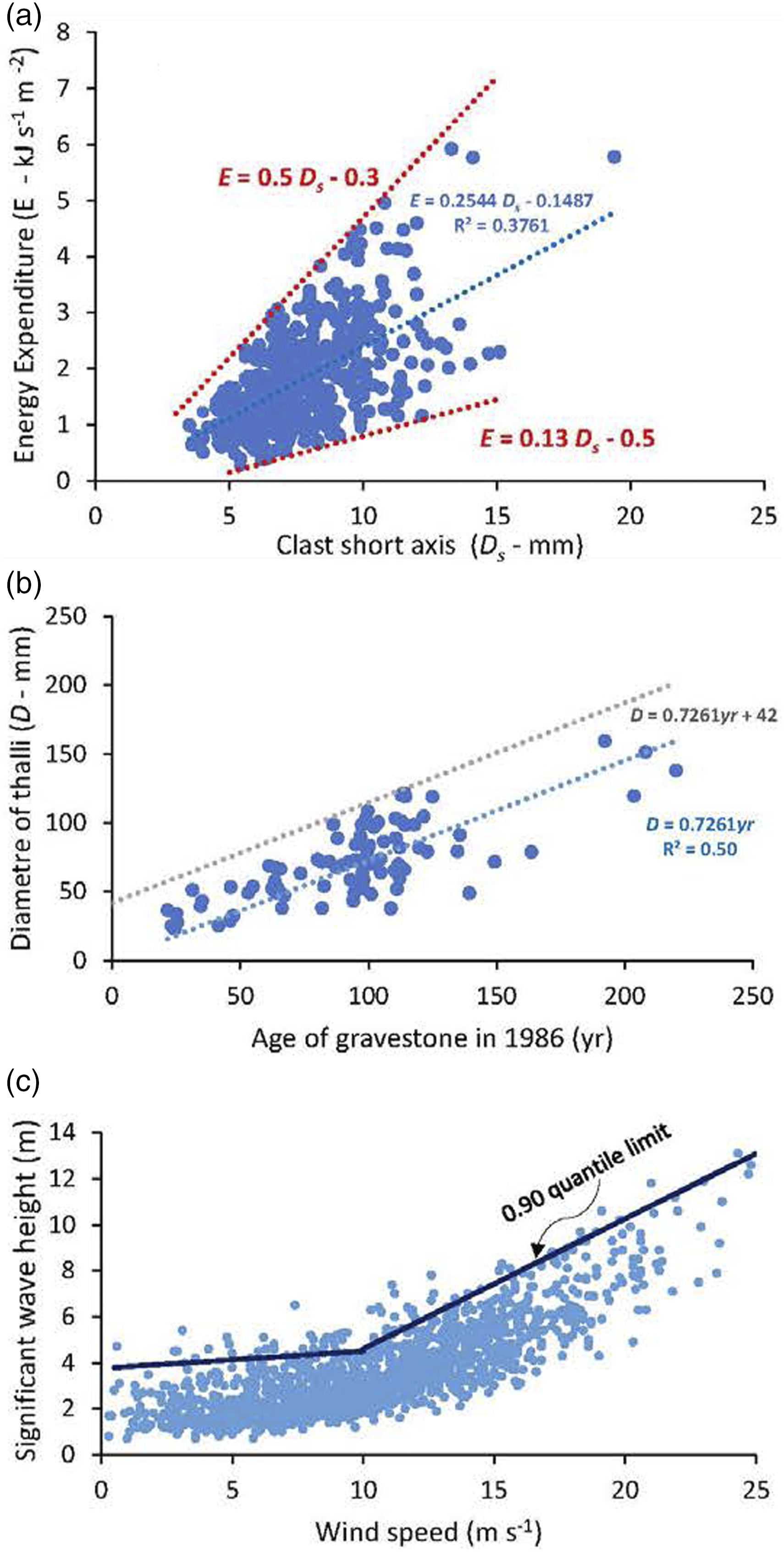

The iterative selective regression procedure of Maller et al. (1983) is an iterative least-squares procedure in which data points are down-weighted according to their distance from a trial line to obtain a new line. This latter line forms the basis for the next iteration. This procedure is equivalent to fitting the least-squares line through an objectively derived sub-set of the data. For consistency with our notation, we refer to this approach as iterative selective regression, although Maller et al. (1983) referred to it as a trimming method. Simulations of the estimates for the iterative selective regression approach show that small biases occur, but the estimates of slope and intercept are approximately normally distributed and are reproducible by other operators. The solution is not uniquely determined, but the accepted fitted line usually is taken to be the solution that includes the greatest number of data points. Carling (1987) used the Maller et al. (1983) method to fit a limit line to define a maximum lichen growth curve. Guidance notes on implementing the Maller et al. (1983) method and an Excel work sheet are archived on Github (Carling et al., 2021).

Parametric model fitting (see Section 2.4.2) is widespread in environmental sciences. Once the parameters of the model have been estimated by fitting to the complete sample, the limit line can be specified and easily calculated, for example in terms of a quantile of the conditional distribution $Y | X = x$ . Fundamental physical and statistical considerations often motivate the choice of parametric model. For example, for count data a Poisson model might be appropriate (see e.g. Chavez–Demoulin and Davison 2005). For measurements of contaminant levels in soils, a log-normal or gamma distribution is often appropriate. The simple linear regression model of Section 2.4.1 is an example of parametric model fitting using a Gaussian assumption. Polynomial models of the form, for example, $Y | (X = x) = a x + b x^{2} + c x^{3} + σ ϵ$ , and response surface models of the form, for example $Y | (X_{1} = x_{1}, X_{2} = x_{2}) = a x_{1} + b x_{2} + c x_{1}^{2} + d x_{2}^{2} + e x_{12} + σ ϵ$ (in terms of two covariates $X_{1}$ and $X_{2}$ ) are also examples of parametric models suitable to define limit lines. Davison and Ramesh (2000), Hall and Tajvidi (2000) and Ramesh and Davison (2002) developed local likelihood models for smoothing sample extremes of single series. Response surface methodology (RSM) is a tool that was introduced in the early 1950s by Box and Wilson (1951). RSM is a collection of mathematical and statistical techniques that is useful for the approximation and optimisation of multivariate stochastic models of 3D surfaces. For example, Shirazi et al. (2020) applied RSM techniques to multivariate data to fit optimal maximum response surfaces related to factors controlling soil erosion using an objective function they termed the desirability function.

Eberhardt and Thomas (1991), considering environmental systems, recommend the Box and Lucas method to obtain optimal parameter estimates of response surfaces; thus, effectively defining limit lines. Box and Lucas is a relatively robust approach but implementation needs a higher level of statistical competency, although software is available to fit a selection of functions (e.g. Originlab^®). The original use was to define a complex curve through few data points which are believed to be the optimal (or in our case maximal) values of $Y$ for given $x$ , to thus assist in choosing further values of $x$ to sample for $Y$ . As new data are added the line is optimised again. The procedure assumes that the trend of the final fitted line defines the outer limit of the region within which data might be expected to occur, or which points are operationally acceptable. Thus, the method is heavily dependent on some prior knowledge of the expected behaviour of maximal values of $Y$ as a function of $x$ . Box and Lucas (1959) did not consider the case where there are many sub-optimal values of $Y$ , which is the focus of this paper. Consequently, there is an issue as to the initial section of points for fitting in cases where many sub-optimal values of $Y$ exist.

Quantile regression (see Section 2.4.3) is capable of modelling any specific quantile of the conditional distribution $Y | X = x$ including the tails (corresponding to say the 95% quantile). However, good performance requires sufficient data to characterise $Y | x$ reasonably as a function of $x$ . To estimate the 95% quantile, we therefore need considerably more than 1/(1–0.95) = 20 observations of $Y$ in the vicinity of each value of $x$ of interest; for the 99% quantile, in excess of 100 observations are required locally for each $x$ . Compared with linear regression, quantile regression is computationally somewhat more demanding, and typically performed using software such as R, PYTHON or MATLAB. Extensions of quantile regression to estimate non-crossing quantiles simultaneously corresponding to different non-exceedance probabilities are computationally more demanding still. Cade (2017) provides an outline of the method for environmental sciences. A simple example is presented as Figure 1(c) and a further example is provided in Supplement 2.

The mixture model of Maller et al., (1983; Kaiser et al., 1994, and see Section 2.4.4) needs a reasonably high level of statistical competency. In outline, values of $Y$ are assumed to be drawn from a mixture of Gaussian distributions. The mean and standard deviation of each mixture component is linearly related to a ‘fullness’ random variable drawn from $[0,1]$ . The mean of each mixture component is also related to $x$ by a linear regression. During inference, a set number of 'fullness’ values is considered, and the parameters of the linear regression and the mixture component from which each particular pair $(x, y)$ are drawn are estimated. The final choice of limit line to adopt given the inference is the choice of the investigator.

Extreme value analysis (see Section 2.4.5) is used widely in environmental science to define return values for processes such as rainfall, temperature, storm, wildfire and earthquake severity, extreme occurrences of which are hazardous. The $T$ -year return value is defined by the equation $P (Y_{A} > y) = 1 / T$ , where $Y_{A}$ is the annual maximum of random variable $Y$ . The distribution of $Y_{A}$ is estimated based on a sample of data using extreme value analysis (see e.g. Coles 2001). The return value can also be defined conditional on a covariate $X$ , as $P (Y_{A} > y | X = x) = 1 / T$ . In this case, a different return value is estimated for each value $x$ of $X$ (see e.g. Davison and Smith 1990). Further details and a software reference are found in Supplement 3.

IV. Practical issues

A number of practical issues arise in attempting to estimate limit lines from a sample of data. In this section, we provide an overview of some of the issues that are likely to be of concern to the practitioner. These include identification of outliers, breakpoints and mixed samples, and the quantification of uncertainty of inference.

4.1. Identifying outliers

In regression modelling (Section 2.4), observations with large residuals (outliers) or high leverage are problematic, since they may violate the assumptions underlying the model and cast doubt on the outcome of a regression. Outlier detection and regression diagnostics naturally have a large statistical literature; the works of Wetherill et al. (1986) and Cook and Weisberg (1982) provide introductions. Traditionally when assessing a dataset before conducting linear regression, outliers were identified by eye from inspection of the x-y scatterplots. Objectively identified outliers likely lie above any proposed limit line so their identification is critical when fitting limit lines.

Unusually large values of $Y$ and $X$ can be identified by examination of extreme quantiles of marginal statistics. Alternatively, if sufficient data for $Y$ occur for a given $x$ , or within some neighbourhood of $x$ , then outliers can be identified from examining histograms of $Y | x$ for each $x$ of interest. Within a linear regression context, model diagnostics such as the diagonal elements of the so-called hat matrix, and Cook’s distance can be used to identify observations with high leverage and influence respectively. Large values of model fit residuals are indicative of outliers. It is also generally useful to examine so-called studentised residuals. These diagnostics are explained in many statistical treatises, and are often included in statistical software packages, so we do not elaborate further.

For joint modelling of bivariate data (Section 2.3), Mahalanobis distance and similar metrics can be used to identify data points which are unusual with respect to that metric. In a regression context, when the occurrence of outliers can be attributed to one or more additional data-generating processes (over and above those responsible for the bulk of the sample), then more sophisticated techniques including mixture modelling can be used to simultaneously estimate ‘bulk’ and ‘outliers’ (e.g. Aitkin and Tunnicliffe Wilson 1980; Yu et al. 2015).

4.2. Identifying breakpoints

It is possible that an attempt to estimate a limit line with given characteristics (e.g. linearity) through x-y data does not yield satisfactory results. If the limit line is estimated using a statistical procedure, then lack of fit can be quantified. In such cases, more general models for the limit line should be sought. The relative performance of different models for the limit line can then be compared, and the best model adopted (e.g. Wetherill et al. 1986). Sometimes it may be appropriate to consider: (1) whether the data might exhibit breakpoints or change-points in the x-y relationship, or; (2) whether a model admitting a non-linear relationship between variates is appropriate (e.g. Zanini et al. 2020). Figure 1(c) illustrates this issue. Here, the slope of the limit line clearly changes at wind speed around 10 ms⁻¹; it might therefore be appropriate to fit a piecewise linear limit line as illustrated. However, physically we know that water waves are generated by the wind via frictional drag forcing, which implies alternative approaches including a linear limit line for y on the square of x, or a quadratic quantile regression limit line might be appropriate. However, the relationship observed at a specific location is unlikely to follow the quadratic form exactly, due to various effects including fetch-limitation, wind-field non-stationarity, bathymetric effects in shallower water etc. For this reason, fitting a piecewise linear form for a limit line is a pragmatically sound way to proceed; in practice, a larger number of piecewise segments might probably be used. In fact, exactly this approach is frequently used in ocean engineering to specify an extreme value threshold, and amounts to an approximate non-parametric quantile regression (see Section 2.4.3).

In general, identifying breakpoints or changepoints in a sample can be important in the interpretation of a physical process (e.g. Ryan et al., 2002). The modelling challenge is to identify one or more breakpoints in $x$ in the sample such that limit lines using data in each of the resulting sub-sets can be estimated more parsimoniously than using the complete sample. Often, prior empirical knowledge, or theory, can be used to locate the breakpoints in terms of x-values. Then separate regression models (or other approaches from Section II) might be adopted for each sub-set to estimate limit lines. When the location of a breakpoint is uncertain, data points close to the expected breakpoint first can be considered to fall into one group and then considered to be part of the other group to influence the regression line trends, thus, repositioning the expected breakpoint.

Identification of breakpoints also can be achieved as part of the statistical inference. For example, optimal partitioning of the x-domain into $K$ intervals, on each of which piecewise constant or piecewise linear regression models are estimated, can be performed (see Ryan et al. 2002, Yang et al. 2016).

4.3. Identifying mixed samples

Sometimes, it is possible that the sample for analysis corresponds to observations of a mixture of different data-generating processes. In this situation, we might expect that limit lines would be more appropriately estimated for the individual processes from which the mixture is composed. It might therefore be useful to perform prior partitioning of the sample into two or more groups using data for both $Y$ and $X$ . This outcome can be accomplished using cluster analysis when there is no prior knowledge of group membership or using one of a large variety of classification techniques (including random forests and support vector machines) when some knowledge of group membership is available. For the two-group case, discriminant analysis (Brereton, 2009; Dixon and Brereton, 2009; Brereton and Lloyd, 2014) is another popular choice. As mentioned in the context of outlier detection above, more sophisticated statistical techniques to model the mixture explicitly can also be employed.

4.4. Quantifying uncertainty

Quantifying the uncertainty of estimates of limit lines is generally important if those estimates are to be trusted. Some of the approaches described in Sections II and III do not involve an explicit quantitative model for the relationship between $Y$ and $X$ ; it is difficult therefore to quantify the uncertainty with which these limit lines are estimated. Other methods from Sections II and III make combined use of a data sample and a statistical model; for these methods and the limit lines they produce, it is therefore possible to quantify uncertainty using well-established approaches.

Sources of model uncertainty can be considered aleatory (due to the inherent natural variation of the process we are modelling, which will always be present) or epistemic (due to inadequate data, measurement procedures, model specification, etc., the effects of which we could in principle eliminate with enough effort).

When a regression-type model for $Y | X = x$ is being estimated, there are broadly two approaches to the quantification of uncertainty. The first approach adopts Bayesian inference. The key steps are (a) specification of full probabilistic data-generating model, (b) specification of a joint prior distribution for all the parameters in the model, (c) estimation of the joint posterior distribution of all parameters by conditioning on a sample of data using Bayes theorem and (d) diagnosing model performance, and estimation of posterior predictive credible intervals for structure variables of interest, such as a limit line. Many statisticians view Bayesian inference as the preferred strategy for model building and decision making, but it often suffers because of the difficulty of specifying reasonable prior distributions for parameters, and the computational complexity of inference. Bishop (2006) and Gelman et al. (2013) provide introductions.

The second approach to uncertainty quantification is based on assessing the variability of inferences from models estimated using resamples of the original data sample. Different resampling techniques, including cross-validation, bootstrapping and randomised permutation testing provide relatively simple pragmatic approaches to estimate the performance of statistical models, to estimate uncertainties of predictions, and perform significance tests. Resampling approaches are widespread in the applied literature, especially when there is some ambiguity about the appropriateness of the model being used. However, some might claim that resampling approaches lack the overall coherence and elegance provided by the Bayesian approach. There is a huge literature on resampling methods; Good (2006) provides an introduction. The works of Molinaro et al. (2005), Hesterberg (2015) and Lehr and Ohm (2017) provide useful practitioner perspectives.

4.5. Measurement error and heteroscedasticity

In many data sets, measurements of both $Y$ and $X$ are made with error. That is, we cannot measure either $Y$ or $X$ precisely. Uncertainty in $Y$ can be accommodated relatively easily in the distributional assumption made for $Y | X = x$ . However, uncertainties in $X$ are more problematic to handle appropriately in simple statistical models. The presence of measurement errors causes increased bias and uncertainty in fitted statistical models, leading to erroneous inferences about limit lines. Using Bayesian inference, we can routinely specify a measurement error model for both $Y$ and $X$ . Alternatively, we can extend conventional regression models to so-called errors-in-variables models.

In a simple linear regression model, we make the assumption that the variance of $Y | X = x$ does not change with the value of $X$ . However, in many applications, this is not the case, and the data are said to exhibit heteroscedasticity. This feature can again be accommodated by extending the regression model.

4.6. Model selection

Model selection is a procedure to select one among many candidate models. Typically, we select a model with the best performance for the task at hand. However, there may be many competing issues relevant for good model selection other than quantitative performance, such as model complexity and interpretability. In many practical situations, a model which is straightforward to estimate, interpretable and gives reasonable performance, is preferrable over a considerably more complex model which is less interpretable and gives only slightly improved performance.

There are essentially two approaches to model selection. In general, probably the wisest approach is based on the assessment of predictive performance of the model, preferring the candidate model with best predictive performance. Predictive performance is assessed by quantifying out‐of‐sample error; that is how well a model performs on data that were not used to fit the model in the first place. There are many approaches to quantifying predictive performance, including (1) partitioning the original data into two groups, using one group to fit a model, and the other group as an unseen test set to estimate predictive performance, and (2) cross-validation, in which the original sample is partitioned into a number of sub-sets which are withheld one at a time, serving as test sets for models estimated using all the remaining sets; an estimate of predictive performance is then accumulated over all the test sets. The second approach to model selection attempts to quantify model performance using fitting performance of the model. However, because fitting performance is typically an over-optimistic assessment of predictive performance, the fitting performance score is usually penalised by a measure of model complexity; more complex models receive higher penalties. A number of related performance measures, including the Akaike Information Criterion (AIC). Bayesian Information Criterion (BIC), and Minimum Description Length (MDL) are available. Pawitan (2001, Sections 13.5–13.6), Davison (2003, Section 4.7) and Kuhn and Johnson (2018, Section 4.8) provide a useful discussion.

V. Examples of current fitting procedures

In this section we make use of three different data sets to illustrate the strengths and weaknesses of fitting limit lines using some of the simpler methods introduced above. For conciseness, we have focussed on those simpler methods. The issues that arise using simpler methods also apply to, and would inform the application of, more advanced statistical procedures. The application here of simpler methods does not imply that more sophisticated approaches could not be explored beneficially in the case of these examples.

The first example consists of a complex of several data sets which, taken together, define a visual upper limit line for which an upper limit is expected from theory. This example is used to demonstrate the use of three relatively simpler methods together with fitting of a theoretical function that makes use of the empirical data.

The second example consists of a single data sets that is inadequate to clearly define a visual upper limit line, although a limit is reasonably expected from prior studies. This example is used to demonstrate the use of three relatively statistically robust methods.

The third example consists of a single data set for which the variance in y increases rapidly as the value of x increases, and both upper and lower limit lines are required. Solutions derived using a simple robust method are contrasted to inspection functions.

Example 1

Catastrophic outburst floods from dammed lakes

Figure 2 serves as an example of the issues that arise from fitting limit lines using Inspection, Selective Regression and application of a data-informed Theoretical Limit. The data sets collectively represent the relationship between measured volumes of released lake water (V) and the estimates of the peak discharge (Q_p) downstream due to catastrophic lake failure (O’Connor et al., 2013). It may be expected that variation in breaching mechanisms, channel geometry and roughness (amongst other controls) will mediate the downstream translation of the flood wave so that different peak discharge values might be obtained for the same initial lake volumes. However, if the discharge from the lake is constrained by the initial geometry of the eroding breach (e.g. critical flow control), or by the way the flood translates down system, there should be an upper limit to the scatter of peak discharge values. The data in Figure 2 considered collectively, or as separate data sets, provide some support for the critical flow control as is detailed below.

Inspection and selective regression: The green curve is fitted by inspection $(Q_{p} = 0.1286 V^{0.83})$ to pass through the three outlying ‘landslide group’ data points. The four green points attract attention because, on log-log coordinates, the four points trace out a straight line lying above the main data spread. Having fitted the green curve, the red ‘constructed group’ data point (lying above the green curve) is defined as an outlier a posteriori, by the simple fact that it lies above the green limit line. Note that this definition of the outlier is unsatisfactory given that robust methods (noted above) are available to determine leverage. All other data points are included within the limit, but forward extrapolation of the limit line means that the curve increasingly deviates away from the observed data. A curve fitted through the four ‘landslide group’ data points (selective regression on a data sub-set), using least-squares regression, provides a similar curve $(Q_{p} = 0.1168 V^{0.83})$ and is preferred to the eye-fitted curve for reasons explained prior.

Selective regression with optimal a*: A least-squares regression of the ‘physical model’ data defines the trend of that data set which, when extrapolated forwards (not shown) passes through the centre of the mass of other data sets. This consilience between the two groups of data suggest that the small-scale model results reproduce well the central tendency of behaviour of large natural dam failures across several orders of magnitude. Interestingly, such an extrapolation might define an upper limit line for ‘Ice dams – subglacial tunnelling’, although we do not explore the implications herein. However, to define a limit line for the majority of data, the trend of the ‘physical model’ data can be adjusted by adding increments to the intercept value, a^∗, until sufficient data points fall below the limit. In the example provided, the intercept value is increased (Selective regression with optimal a^∗) by a factor of ten such that although ten data points lie outside the limit, the black line provides a reasonably satisfactory visible limit to the data spread, notably that of the ‘constructed group’ and ‘moraine group’ data sets. A small increase in the intercept value would readily include seven more data points leaving only three as outliers. By adjusting the intercept value, the exponent of the trend line is preserved, implying that the central tendency growth function for ‘physical model’ data also can define the behaviour of data at the upper limit to the larger-scale dam-break data. By such systematic exploration of central tendency and limits, consideration can be given to (i) the relationship of one data set to another; and (ii) the consistency of data point plotting positions within the individual data sets. Further, (iii) the positions of some individual data points come under scrutiny and; (iv) possible theoretical constraints on the data plotting positions may become evident.

Theoretical Limit: A theoretical critical flow control might be considered to provide an upper limit to the data spread in Figure 2. The theoretical derivation is provided as Supplement 1 but the basic facts are as follows. Failure of earthen and ice dams often is associated with initial establishment of a critical-flow depth (h_c) at the breach that determines the peak outflow discharge (Walder and O’Connor, 1997; O’Connor and Beebee, 2009). Larger volume (V) lakes tend to have greater depths (h) and so have the propensity to develop rapid failures with greater critical flow depths; thus, h_c $\propto$ h. Assuming that the outflow breach, and thus the critical flow depth, will be larger for larger water bodies, the maximum discharge Q_p should be proportional to the lake volume efflux (V). O’Connor and Beebee (2009) showed that a critical flow control can be approximated as

Q_{p} = p g^{\frac{1}{2}} {h_{c}}^{\frac{5}{2}}

(1)

where g is the acceleration due to gravity and p is a proportionality coefficient.

The V-data in Figure 2 are used to calculate $Q_{p}$ , so defining the values of h_c and p in equation (1) can be seen as a fitting procedure, rather than just adding a theoretical function to the graph. Equation (1) provides a theoretical basis for the slope (b) of the green limit line. The slope of equation (1) is practically coincident with both the line drawn by inspection and the least-squares power function (b = 0.83) obtained using selective regression on a data sub-set (as reported above), matching the position of these two curves when p = 1.0. It is beyond the scope of this paper to discuss the reasons why the limit line constructed using theory has a steeper gradient than that devised using selective regression with optimal a*. Nevertheless, fitting the various limit lines leads to considerations such as that the theory applied may be too restrictive, or the small-scale physical model data may not adequately represent larger natural systems.

Figure 2.

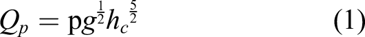
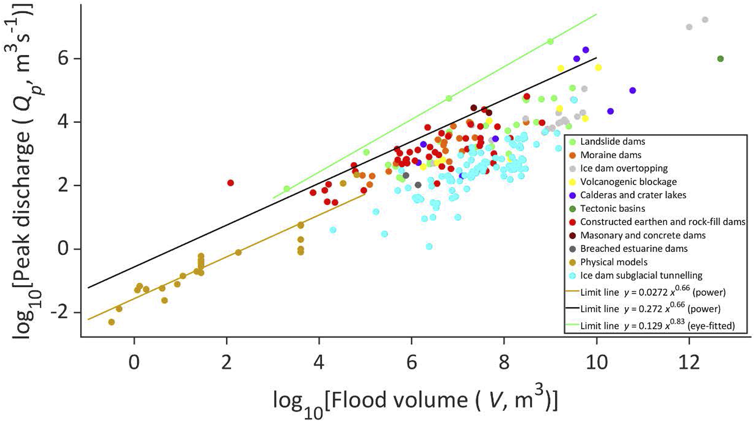
Empirical data define the relationship between the flood volume and the peak discharge of water released from catastrophic failures of dammed lakes. Brown curve is the least-squares fit to the physical model data; Limit line (black) fitted to all the data using selective regression with optimal a*; Limit line (green) fitted by inspection of a data sub-set. The equivalent theoretical equation, $Q_{p} = g^{\frac{1}{2}} {(h_{c})}^{5.2}$ , is essentially the same as the green line (see main text).

Example 2

Lichen growth curve to date flood deposits

Figure 3 serves as an example of the issues that arise from fitting limit lines using parametric mixture modelling. The data considered (Carling, 1987) define the relationship between the diameter of the largest lichen thalli on dated gravestones in Teesdale, northern England (Figure 1(b)). Such lichen growth curves can be used to date the surface of rocks that have been transported by floods or glaciers in the same region for which the calibration data were obtained. The supposition is that geophysical flows transport, abrade and destroy any pre-existing lichens, such that lichen growth only occurs once the rocks are stable in a deposit. In this manner, flood gravel bars can be dated. The species of lichen (Huilia albocaerulescens) used by Carling (1987) tends to produce circular thalli which, after an initial rapid growth phase of a few years only, tend to steadily increase linearly in size with age. Eventually lichens reach senescence, at which time lichen thalli cease to grow, grow more slowly, or being to break-up. Consequently, any maximum linear growth function can only be extended to a given x:y breakpoint value beyond which maximum growth does not apply (Cooley et al. 2006). Beyond this point, either a separate lower-gradient function is fitted for the senescence phase, or, if a single function is fitted it must account for the growth and senescence phases (Innes, 1983). In ideal growth conditions, lichens will achieve a maximum diameter during the rapid growth phase. Data scatter occurs below an expected upper limit to the x:y data pairs occurs for a number of reasons, including: pollution, the date on the gravestone being added some time after erection; differences in the rock type, aspect, and occasional cleaning of gravestones.

Box and Lucas: The data shown in Figure 3 produces an upper limit line (blue curve) when using the Originlab^® procedure, that is of the same form as a conventional least-squares exponential fit (orange curve) through all the data. Both curves are constrained to have an origin at T equals zero, although other intercepts could be specified. A linear least-squares zero-intercept fit to all the T ≤ 190 data pairs (not shown), to represent only the growth phase, statistically would be a less good fit (r² = 0.31) than the orange curve. The fitted limit is that which maximises the r² value for eight outer points, so other curves could be selected if desired. The points that lie just above the D_max exponential solution were determined to do so by the final choice of the curved fitted. The fitted line intuitively is acceptable as it encloses 93% of the data points, but a higher curve could equally be obtained to enclose more data points.

Mixture modelling: An expectation–maximisation (EM) algorithm was used to fit the red curve in Figure 3 following the mixture model of Maller et al. (1983). The least-squares trimming method of Maller et al. (1983) leads to a solution (green curve) that is similar to selective regression (which fits a least-squares function to an arbitrary selection of data points), but the degree of objectivity in curve fitting is greater using mixture modelling. The solution is not uniquely determined, but the accepted fitted line usually is taken to be the solution that includes the greatest number of data points. In the case of the data in Figure 3, a limit was derived after eight iterations which enclosed 95% of all data points and which passes through a further 4% leaving two points just above the curve. The fitted curve: D_max = 0.815T + 24.33 lies slightly below the red curve fitted using EM algorithm which enclosed all data points.

As lichens often exhibit initial rapid growth, followed by a linear growth phase, followed by an exponential decline during senescence (Cooley et al. 2006), a bipartite or tripartite limit line might be preferable, although in the case of the data in Figure 3 there are inadequate data to define a separate senescence phase. However, it would be more satisfying if recourse was made to biologically based theoretical models of lichen growth (Childress and Keller, 1980) to determine what form of function should be fitted that mimics the growth of lichens.

Figure 3.

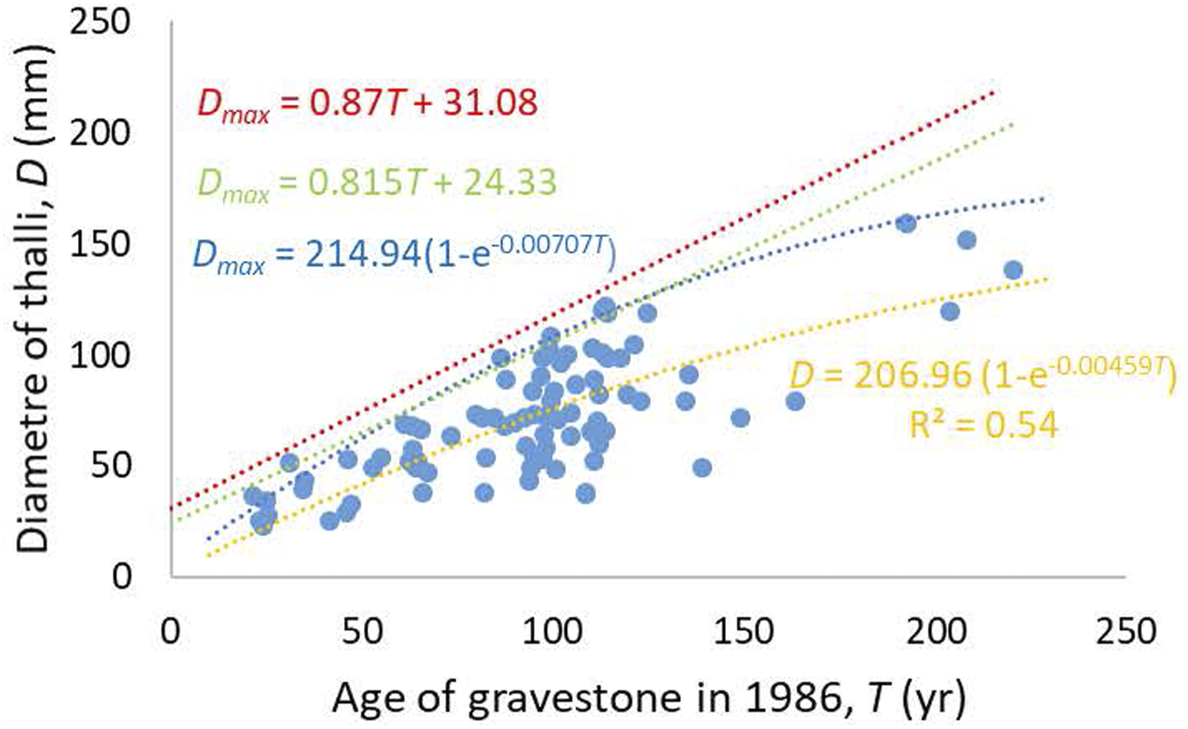
Empirical relationship between the date on gravestones and the diameter of lichen thalli in 1986. Data from Carling (1986). The red curve was fitted using an EM algorithm. The green curve was fitted using the Maller et al. (1983) trimming method. The blue curve was fitted using the Box and Lucas (1959) method. The orange curve was fitted to all the data using a least-squares exponential fit.

Example 3

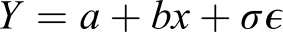
Variation in energy expenditure required to fracture pebbles

Figure 4 serves as an example of the issues that arise from fitting limit lines using Inspection and Iterative Selective Regression. Figure 4 reproduces the data shown in Figure 1(a), with additional limit lines fitted. The data published originally by Tuitz et al. (2012) were presented in this graphical context by Carling and Fan (2020). The data represent the variation in experimentally derived energy expenditures recorded using a laboratory point-load test to fracture river pebbles. It is known from theory and empirical measurements in prior published studies of facture processes that the energy should increase in a linear manner for the range of pebble sizes considered here. However, as pebble size increases the number and complexity of flaws in the pebbles also increases such that the variance in the y data increases as a function of x. Carling and Fan (2020) only wished to draw attention to the data spread and eye-fitted the red-dotted lines to delimit the data spread. The lower and upper blue fitted limit lines were obtained after seven and nine iterations respectively using iterative selective regression.

Figure 4.

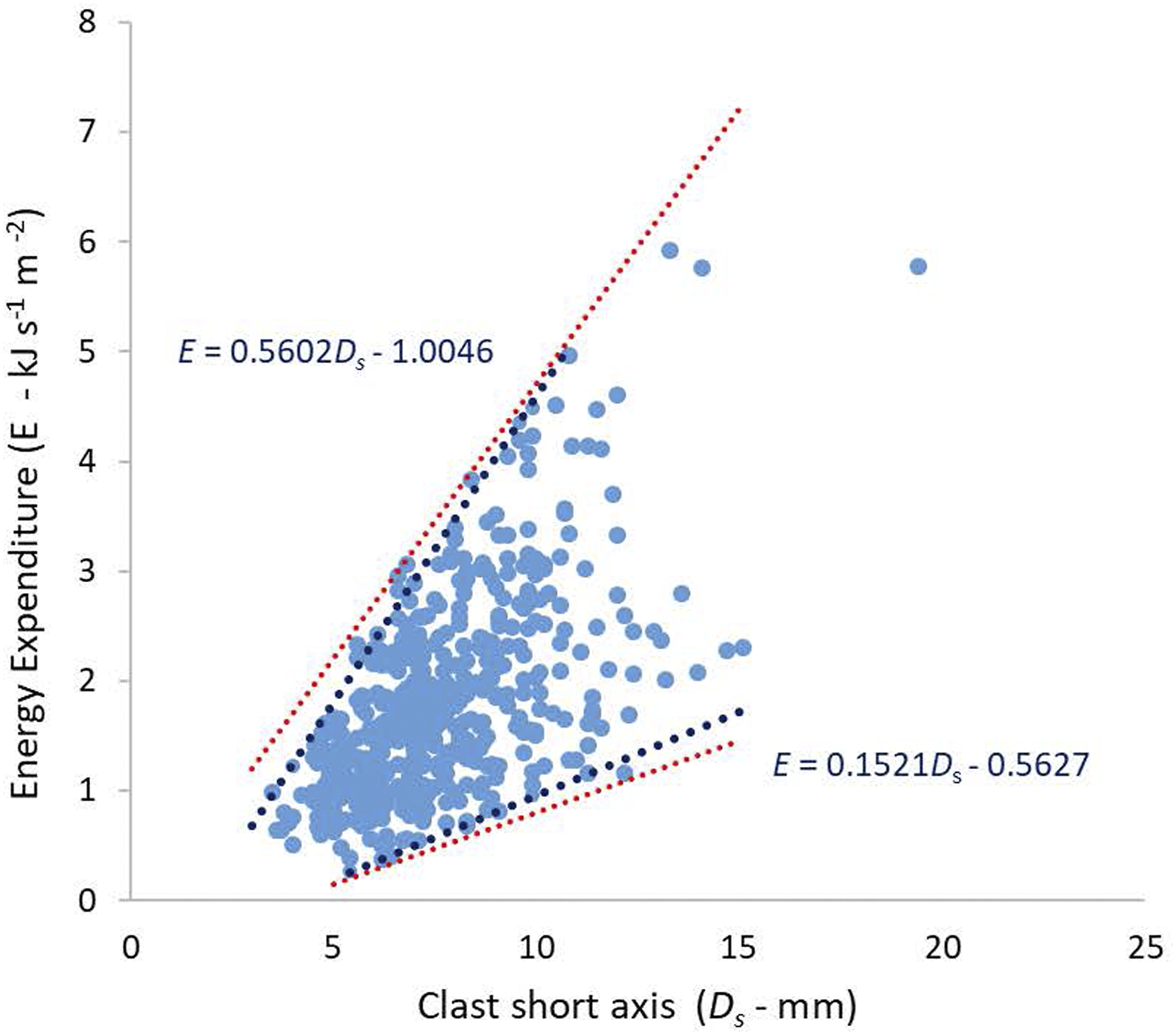
Variation in experimentally derived energy expenditures recorded using point-load test applied to fracture water-worn pebbles. Red curves were fitted by visual inspection. Blue curves were fitted using selective regression.

6. Concluding Discussion

Researchers sometimes wish to define boundaries, upper or lower limits to samples of data, and hence to the distributions from which those samples are drawn. In choosing an approach to achieve this, the researcher should be as specific as possible about the objective of their data analysis. Consideration should be given as to how the inferences derived from the analysis will be used further to inform decisions. In some fields, including hydrology and environmental engineering, there are specific concerns regarding characterisation of extreme values of the data-generating process. In these areas, techniques motivated by extreme value theory are relatively commonplace to quantify the (joint) tails of distributions from samples, and to estimate extreme quantiles including upper bounds for conditional distributions such as $Y | x$ . However, in many other fields, estimation of boundaries or limit lines has received little or no attention. Rather weak ad-hoc methods, making limited use of available data and quantitative modelling, have been applied. On occasion, statistical methods such as linear regression, devised to characterise the general nature of data spread $Y | x$ have been adapted to locate possible limit lines. Rarely have statistical approaches which specifically seek to characterise the tail $Y | Y > u, x$ been used. Often a limited number of observations precludes statistical modelling. Specifically, for the applications illustrated in Figures 1(b)–4, sample size is sufficient to attempt relatively simple regression models for $Y | x$ , including quantile regression; however, it would not be feasible to quantify the conditional tail $Y | Y > u, x$ using extreme value analysis. Sometimes, weaker ad-hoc methods are adopted because of a lack of awareness or appreciation that more principled approaches may be useful. In general, ad-hoc methods should not be used in cases where more principled statistical procedures can be applied, because the latter are clearly defined mathematical models making use of available data, are reproducible and allow quantification of uncertainty. Whereas ad-hoc methods introduce uncertainty with respect to interpretation, adoption of statistical procedures allows both authors of articles and readers to further explore the implications of the fitted functions in a rational manner.

In the absence of theoretical knowledge as to the form of a limit line, the qualitative procedure of inspection is a useful initial means to consider the likely form of a function. Indeed, the intuitive understanding of how the data behaves can assist in statistical model formulation, yet at the same time inspection can lead to false inferences as to the likely behaviour of a limit. The quantitative nature of data allows objective fitting of a statistical function, which can then be compared with the intuitive expectations of the analyst. Given that a variety of statistical models are available, it is important to consider at the outset the purpose of the fitting exercise and to choose the method that is most appropriate to satisfy the objective. Fitting statistically derived limit lines is especially powerful in those cases where the theoretical limit is either well-known or the behaviour is reasonably expected. In these cases, the close agreement of the statistically fitted limit with a theoretically derived line can be confirmatory. In contrast, significant discrepancies between the two curves may indicate deficiencies with the data sample: additional data may be required, or the quality of existing data may be suspect. Discrepancies may also highlight theoretical or model inadequacies: the possibility that other covariates are affecting y- or x-values, or that the theory may need revision.

In the examples provided herein (section V) it is evident that the application of different methods produces different limit lines. In some applications, these discrepancies may not be significant. As previously noted, the identification of extreme behaviour within environmental systems can be very important for instance in hazard mitigation. In such critical situations, the development of limit lines rationally informed by empirical evidence, statistical and physical theory is preferable. Although this conclusion may seem obvious, there are many examples in the literature of limit lines fitted without consideration of existing theory. For example, surprisingly, limit lines are often fitted to define the relationship between the maximum flood discharges generated from given catchment areas without consideration of the maximum probable flood (MPF). The MPF is the theoretical expectation (e.g. Shalaby, 1994; USFERC, 2001) and it would be informative to compare the statistically derived flood limit lines with the theoretical functions. Where theory is unavailable, consideration should be given as to whether the application of different methods tends to lead to convergence in terms of the form and trend of several limit lines. In general, however, identifying the sub-set of methods that provide consistent estimates of limit lines is likely only to be possible once the details of the problem and data have been understood. Building an appreciation for the relative performance of different methodologies via simulation study for a specific problem type is useful and standard practice in the statistics literature. However, the number of potential problem types is huge, and therefore the specifics of the problem of interest first need to be clearly defined before the simulation study is undertaken.

The use of advanced statistically methods in contrast to simple ones readily can be justified (Jomelli et al. 2010), especially when there is plentiful empirical evidence. Not least, given the inevitable ambiguity in fitting of limit lines, it is important to reason systematically whilst recognising the uncertain evidence that even large data sets offer (e.g. using Bayesian analysis). However, situations occur where the x-y data points are few, or their disposition on the scatter plot render the application of sophisticated methods impracticable or impossible. Such situations usually indicate that additional data are required, or that stronger assumptions about the data-generating process are necessary. Regardless, the procedure used to fit a limit line should be documented sufficiently clearly that limit line estimation given a sample of data can be reproduced with confidence. Fitting a limit by Inspection alone rarely can be justified.

The advantage of a statistical approach in general is that it provides a rational, reproducible basis for inference, and hence a sound basis for learning: different practitioners working independently can be reasonably expected to make the same inference given a sample of data. The performance of a model is dependent on the quality of information used to infer it. It is not reasonable in general to expect that a statistical model provides a ‘better result’ than a visual fit, since a well-informed visual fit may be superior to a badly specified statistical model. However, it is also self-evident than an ill-informed visual fit can lead to spectacularly bad inferences.

The outline taxonomy or road map provided in Section II provides an overview of the range of statistical methodologies available for estimation of limit lines, and references to statistical texts which explain methodologies in more detail. Choice of the appropriate methodology will be problem specific. When dealing with an unfamiliar problem, seeking the advice of a statistician is likely to be beneficial. Given the uncertainty that can pertain to model fitting, we conclude by providing some signposts that may assist in the decision-making process of limit line fitting:

• Define the objective of the analysis: for what purpose will the fitted limit line be used? Consider how this informs the analysis to be undertaken

• Assess the data to hand, the characteristics of the measurement used to gather data, and likely sources of uncertainty. Are the measurements independent (given covariates)? Are the data representative? What is the potential for gathering further relevant data?

• Determine if theory allows the form of the limiting function to be defined

• Determine whether a statistical model can be adopted for the data-generating process and fitted to the data. Limit lines may then be estimated using the fitted statistical model. What form of statistical model is likely to be more appropriate? Otherwise consider what form of limit line curve might be appropriate from knowledge of the system behaviour

• Assess the appropriate level of sophistication of the statistical model or limit line curve, guided by parsimony. Is it likely that (unknown, unmeasured) covariates are in play? Should breakpoints be considered?

• In fitting the statistical model or limit line, always assess fitting performance using diagnostic plots and tools. Assess potential outliers.

• Seek to quantify uncertainties in the fitted model (line), and propagate those uncertainties to subsequent decisions made using the fitted model (line)

Supplemental Material

sj-pdf-1-ppg-10.1177_03091333211059995 – Supplemental Material for Fitting limit lines (envelope curves) to spreads of geoenvironmental data

Supplemental Material, sj-pdf-1-ppg-10.1177_03091333211059995 for Fitting limit lines (envelope curves) to spreads of geoenvironmental data by Paul A Carling, Philip Jonathan and Teng Su in Progress in Physical Geography: Earth and Environment

Supplemental Material

sj-jpg-2-ppg-10.1177_03091333211059995 – Supplemental Material for Fitting limit lines (envelope curves) to spreads of geoenvironmental data

Supplemental Material, sj-jpg-2-ppg-10.1177_03091333211059995 for Fitting limit lines (envelope curves) to spreads of geoenvironmental data by Paul A Carling, Philip Jonathan and Teng Su in Progress in Physical Geography: Earth and Environment

Footnotes

Acknowledgements

Teng Su acknowledges the receipt of China Postdoctoral Science Foundation Grant No. 2020M670435. Software for the trimming method of Maller et al. (1983) is provided at Carling et al. (2021), and for simple non-stationary extreme value analysis at . We are grateful to the Editor, Karen Anderson and two anonymous reviewers for their comments which substantially improved the presentation of the results.

Declaration of conflicting interests

The author(s) declared no potential conflicts of interest with respect to the research, authorship and/or publication of this article.

Funding

The author(s) received no financial support for the research, authorship and/or publication of this article.

ORCID iD

Paul A Carling

Supplemental Material

Supplemental material for this article is available online.

References

Aitkin

Wilson

(1980) Mixture models, outliers and the EM algorithm. Technometrics 22: 325–331.

Bagnold

(1966) An approach to the sediment transport problem from general physics. U.S. Geological Survey Professional Paper 422-1, p. 37.

Bagnold

(1980) An empirical correlation of bedload transport rates in flumes and natural rivers. Proceedings of the Royal Society of London, A 372: 453–473.

Bishop

(2006) Pattern Recognition and Machine Learning. New York: Springer.

Box

GEP

Wilson

(1951) On the experimental attainment of optimum conditions. Journal of the Royal Statistical Society, Series B 13: 1–38.

Box

GEP

Lucas

(1959) Design of experiments in non-linear situations. Biometrika 46: 77–80.

Brereton

(2009) Chemometrics for Pattern Recognition. Chichester: John Wiley and Sons.

Brereton

Lloyd

(2014) Partial least squares discriminant analysis: taking the magic away. Journal of Chemometrics 28: 213–225.

Cade

(2017) Quantile regression applications in ecology and the environmental sciences. In: Koenker

, et al. (eds) Handbooks of Modern Statistical Methods: Handbook of Quantile Regression. London, UK: Chapman & Hall/CRC, 429–454.

10.

Carling

(1987) Lichenometric dating applied to flood deposits. In: Beschta

Blinn

Grant

, et al. (eds) Proceedings of a Symposium on Erosion and Sedimentation in the Pacific Rim. Corvallis: International Association of Hydrological Sciences, 395–396.

11.

Carling

(1989) Bedload transport in two gravel-bedded streams. Earth Surface Processes and Landforms 14: 27–39.

12.

Carling

Fan

(2020) Particle comminution defines megaflood and superflood energetics. Earth-Science Reviews 204: 103087

13.

Carling

Jonathan

Teng

(2021) Spreadsheet software for the trimming method of Maller et al. (1983). https://github.com/ygraigarw/LimitLines

14.

Castellarin

(2007) Probabilistic envelope curves for design flood estimation at ungauged sites. Water Resources Research 43: W04406. DOI:10.1029/2005WR004384

15.

Chavez-Demoulin

Davison

(2005) Generalized additive modelling of sample extremes. Journal of Royal Statistical Society Series C: Applied Statistics 54: 207–222.

16.

Childress

Keller

(1980) Lichen growth. Journal of Theoretical Biology 82: 157–165.

17.

Coles

(2001) An Introduction to Statistical Modeling of Extreme Values. New York: Springer.

18.

Cook

Weisberg

(1982). Residuals and Influence in Regression. London, UK: Chapman and Hall.

19.

Cooley

Naveau

Jomelli

, et al. (2006) A Bayesian hierarchical extreme value model for lichenometry. Environmetrics 17: 555–574.

20.

Davison

(2003) Statistical Models. Cambridge, UK: Cambridge University Press.

21.

Davison

Ramesh

(2000) Local likelihood smoothing of sample extremes. Journal of the Royal Statistical Society 62: 191–208.

22.

Davison

Smith

(1990) Models for exceedances over high thresholds. Journal of the Royal Statistical Society 52: 393–493.

23.

Dixon

Brereton

(2009) Comparison of performance of five common classifiers represented as boundary methods: euclidean distance to centroids, linear discriminant analysis, quadratic discriminant analysis, learning vector quantization and support vector machines, as dependent on data structure. Chemometrics and Intelligent Laboratory Systems 95: 1–17.

24.

Eberhardt

Thomas

(1991) Designing environmental field studies. Ecological Monographs 61: 53–73.

25.

Gaume

Bain

Bernardara

, et al. (2009) A compilation of data on European flash floods. Journal of Hydrology 367: 70–78.

26.

Gelman

Carlin

Stern

, et al. (2013) Bayesian Data Analysis. 3rd edition. USA: Chapman and Hall/CRC.

27.

Good

(2006) Resampling Methods: A Practical Guide to Data Analysis. Basel, Switzerland: Birkhauser.

28.

Hall

Tajvidi

(2000) Nonparametric analysis of temporal trend when fitting parametric models to extreme-value data. Statistical Science 15: 153–167.

29.

Hao

Naiman

(2007). Quantile Regression. London: Sage Publications.

30.

Hesterberg

(2015) What teachers should know about the bootstrap: resampling in the undergraduate statistics curriculum. American Statistician 69: 371–386.

31.

Innes

(1983) Development of lichenometric dating curves for Highland Scotland. Transactions of the Royal Society of Edinburgh: Earth Sciences 74: 23–32.

32.

Joe

(2014) Dependence Modelling with Copulas. Boca Raton, FL, USA: CRC Press.

33.

Jomelli

Naveau

Cooley

, et al. (2010) A response to Bradwell’s commentary on “recent statistical studies in lichenometry”. Geografiska Annaler: Series A, Physical Geography 92:485–487.

34.

Jonathan

Ewans

(2021) MATLAB Code for Simple Non-Stationary Extreme Value Analysis, Estimated Using MCMC. https://github.com/ygraigarw/SimpleNonstationaryExtremesBayesian.

35.

Kaiser

Speckman

Jones

(1994) Statistical models for limiting nutrient relations in inland waters. Journal of the American Statistical Association 89: 410–423.

36.

Koenker

(2005). Quantile Regression. New York: Cambridge University Press.

37.

Kuhn

Johnson

(2018). Applied Predictive Modeling. New York: Springer.

38.

Lehr

Ohm

(2017) Playing with the data: what legal scholars should learn about machine learning. U C Davis Law Review 51: 653–717.

39.

Maller

de Boer

Joll

, et al. (1983) Determination of the maximum foregut volume of Western Rock Lobsters (Panulirus cygnus) from field data. Biometrics 29: 543–551.

40.

McLachlan

Lee

Rathnayake

(2019) Finite mixture models. Annual Review of Statistics and Its Application 6: 355–378.

41.

Molinaro

Simon

Pfeiffer

(2005) Prediction error estimation: a comparison of resampling methods. Bioinformatics 21: 3301–3307.

42.

O’Connor

Beebee

(2009) Floods from natural rock-material dams. In: Burr

Carling

Baker

(eds) Megaflooding on Earth and Mars. Cambridge, UK: Cambridge University Press, pp. 128–171.

43.

O’Connor

Clague

Walder

, et al. (2013) Outburst floods. In: Shroder

Wohl

(Volume Editor). Treatise on Geomorphology, Vol 9, Fluvial Geomorphology, San Diego: Academic Press, 475–510.

44.

Pawitan

(2001) In All Likelihood: Statistical Modelling and Inference Using Likelihood. UK: OUP Oxford.

45.

Ramesh

Davison

(2002) Local models for exploratory analysis of hydrological extremes. Journal of Hydrology 256: 106–119.

46.

Reistad

Breivik

Haakenstad

, et al. (2011). A high-resolution hindcast of wind and waves for the North Sea, the Norwegian Sea, and the Barents Sea. Journal of Geophysical Research 116: 1–18.

47.

Ross

Astrup

Bitner-Gregersen

, et al. (2020). On environmental contours for marine and coastal design. Ocean Engineering 195: 106194.

48.

Ryan

Porth

Troendle

(2002) Defining phases of bedload transport using piecewise regression. Earth Surface Processes and Landforms 27: 971–990.

49.

Shalaby

(1994) Estimating probable maximum flood probabilities. Journal of the American Water Resources Association 30: 307–318.

50.

Shirazi

Khademalrasoul

Ardebili

SMS

(2020) Multi-objective optimization of soil erosion parameters using response surface method (RSM) in the Emamzadeh watershed. Acta Geophysica 68: 505–517.

51.

Tarolli

Borga

Morin

, et al. (2012) Analysis of flash flood regimes in the North-Western and South-Eastern Mediterranean regions. Natural Hazards and Earth System Sciences 12: 1255–1265.

52.

Tuitz

Exner

Frehner

, et al. (2012) The impact of ellipsoidal particle shape on pebble breakage in gravel. International Journal of Rock Mechanics & Mining Sciences 54: 70–79.

53.

USFERC (2001) United States federal energy regulatory commission, 2001. Determination of the probable maximum flood (Chap. VIII). In Engineering Guidelines for the Evaluation of Hydropower Projects. Washington (DC): United States Department of Energy, 121.

54.

Walder

O’Connor

(1997) Methods for predicting peak discharge of floods caused by failure of natural and constructed earthen dams. Water Resource Research 33: 2337–2348.

55.

Wetherill

Duncombe

Kenward

, et al. (1986) Regression Analysis with Applications. Dordrecht: Springer.

56.

Yang

Liu

Tsoka

, et al. (2016) Mathematical programming for piecewise linear regression analysis. Expert Systems with Applications 44: 156–167.

57.

Chen

Yao

(2015) Outlier detection and robust mixture modeling using nonconvex penalized likelihood, Journal of Statistical Planning and Inference 164: 27–38.

58.

Zanini

Eastoe

Jones

, et al. (2020) Covariate representations for non-stationary extremes. Environmetrics 31: e2624.

Supplementary Material

Please find the following supplemental material available below.

For Open Access articles published under a Creative Commons License, all supplemental material carries the same license as the article it is associated with.

For non-Open Access articles published, all supplemental material carries a non-exclusive license, and permission requests for re-use of supplemental material or any part of supplemental material shall be sent directly to the copyright owner as specified in the copyright notice associated with the article.

0.00 MB

0.11 MB

0.45 MB

Fitting limit lines (envelope curves) to spreads of geoenvironmental data

Abstract

Keywords

1. Introduction

1.1. Overarching objective of the data analysis

II Approaches to limit line estimation – a statistician view

2.1. Inspection

2.2. Theoretical limit

2.3. Joint statistical models

2.4. Conditional statistical models for Y | x

2.4.1. Linear regression

2.4.2. Parametric model

2.4.3. Non-parametric model

2.4.4. Mixture model

2.4.5. Conditional models for Y | Y > u ( x ) , x

III Approaches to limit line estimation – a practitioner view

IV. Practical issues

4.1. Identifying outliers

4.2. Identifying breakpoints

4.3. Identifying mixed samples

4.4. Quantifying uncertainty

4.5. Measurement error and heteroscedasticity

4.6. Model selection

V. Examples of current fitting procedures

6. Concluding Discussion

Supplemental Material

sj-pdf-1-ppg-10.1177_03091333211059995 – Supplemental Material for Fitting limit lines (envelope curves) to spreads of geoenvironmental data

Supplemental Material

sj-jpg-2-ppg-10.1177_03091333211059995 – Supplemental Material for Fitting limit lines (envelope curves) to spreads of geoenvironmental data

Footnotes

Acknowledgements

Declaration of conflicting interests

Funding

ORCID iD

Supplemental Material

References

Supplementary Material

2.4. Conditional statistical models for $Y | x$

2.4.5. Conditional models for $Y | Y > u (x), x$