
Abstract
Repeat observations underpin our understanding of environmental processes, but financial constraints often limit scientists’ ability to deploy dense networks of conventional commercial instrumentation. Rapid growth in the Internet-Of-Things (IoT) and the maker movement is paving the way for low-cost electronic sensors to transform global environmental monitoring. Accessible and inexpensive sensor construction is also fostering exciting opportunities for citizen science and participatory research. Drawing on 6 years of developmental work with Arduino-based open-source hardware and software, extensive laboratory and field testing, and incorporation of such technology into active research programmes, we outline a series of successes, failures and lessons learned in designing and deploying environmental sensors. Six case studies are presented: a water table depth probe, air and water quality sensors, multi-parameter weather stations, a time-sequencing lake sediment trap, and a sonic anemometer for monitoring sand transport. Schematics, code and purchasing guidance to reproduce our sensors are described in the paper, with detailed build instructions hosted on our King’s College London Geography Environmental Sensors Github repository and the FreeStation project website. We show in each case study that manual design and construction can produce research-grade scientific instrumentation (mean bias error for calibrated sensors –0.04 to 23%) for a fraction of the conventional cost, provided rigorous, sensor-specific calibration and field testing is conducted. In sharing our collective experiences with build-it-yourself environmental monitoring, we intend for this paper to act as a catalyst for physical geographers and the wider environmental science community to begin incorporating low-cost sensor development into their research activities. The capacity to deploy denser sensor networks should ultimately lead to superior environmental monitoring at the local to global scales.
Keywords
I Introduction
1.1 Hurdles to environmental monitoring
Environmental science is rooted in observation. Long-term measurements of ecological, meteorological and hydrological variables provide the foundation for understanding trends, establishing benchmarks and informing policy (Mishra and Coulibaly, 2009; Tetzlaff et al., 2017). Such data are critical for estimating magnitudes of change in natural systems induced by human activity, such as projected climate warming (Hannah et al., 2011). Although the ever-increasing sophistication of remote sensing tools and computational models is delivering major advances in environmental science (McCabe et al., 2017), gaps in on-the-ground observations are constraining predictive models (Urban et al., 2016). Indeed, whilst data gathering by satellites expands, there has been a concurrent shrinking of conventional ground-based monitoring and measurement for many environmental systems. Appetite amongst funding agencies to support long-term environmental monitoring networks is diminishing (Tetzlaff et al., 2017) and experimental and field research in the hydrological sciences, for example, are in decline (Burt and McDonnell, 2015). The global density of river gauging stations has decreased since the 1980s (Global Runoff Data Centre, 2018; Hannah et al., 2011) and similar rates of closure of hydrometeorological stations, especially in Africa and Latin America (Overeem et al., 2013; World Meteorological Organization [WMO], 2009, cited in van de Giesen et al., 2014), have been shown to hamper ground-truthing efforts (Lorenz and Kunstmann, 2012). This trend is concerning since satellite remote sensing is not without limitations, including the mismatch in spatial and temporal scales between satellite observations and environmental phenomena. For example, the coarse spatial resolution of current satellite soil-moisture products does not adequately capture fine-scale variability (Larson et al., 2008; Tebbs et al., 2019). In addition, several parameters cannot be directly measured from satellite remote sensing (e.g. sub-surface soil moisture or dissolved oxygen; DO). In situ measurements are therefore essential for obtaining a more complete understanding of environmental processes, validating satellite products and improving model projections (e.g. Urban et al., 2016).
Time and financial expense are major barriers to collecting ground-based environmental data (Muller et al., 2015; Tauro et al., 2018). Sophisticated instrumentation brings high maintenance costs and a continual need for skilled staff. Increasing the spatial and temporal resolution of repeat measurements demands proportionally greater allocation of resources. Many legally mandated international monitoring schemes however suffer logistical constraints. The EU Water Framework Directive, for example, requires member states to measure river water quality four times per year, but summed annual loadings are almost certainly underestimates with wide margins of error (Skarbøvik et al., 2012). Public health concerns are promoting investment in air quality monitoring networks in some regions (Environmental Defense Fund, 2018; United Nations Environment Programme, 2020) but networks of high-cost fixed sensors may lack the granularity to pinpoint emission hotspots or their sources, assess the influence of localised meteorology or track pollution plumes (Castell et al., 2017; Morawska et al., 2018; Rai et al., 2017; Thompson, 2016). Though modelling can go some way to filling the void, models such as atmospheric dispersion models are computationally heavy and limited in their predictive capabilities (Kumar et al., 2015).
Alternative monitoring approaches using innovative technology are gaining momentum across the environmental sciences (Bramer et al., 2018; Muller et al., 2015; Tauro et al., 2018). The use of bioacoustic monitoring for wildlife research and biodiversity conservation has surged in popularity and is showing great promise, for example (e.g. Browning et al., 2017; Teixeira et al., 2019). Low-cost, build-it-yourself instrumentation is also becoming increasingly popular (Kumar et al., 2015; Mao et al., 2019; Mickley et al., 2019), enabling much finer-scale environmental data to be collected both spatially and temporally (Horsburgh et al., 2019). Low-cost sensor networks have been shown to improve the spatial coverage of ground-truthing data for validating satellite products (Tebbs et al., 2019) and some large-scale hydrometeorological monitoring networks have been launched, including the FreeStation initiative (www.freestation.org) and the Trans-African HydroMeteorological Observatory (www.tahmo.org; van de Giesen et al., 2014). Alongside these research avenues, open-source development communities such as the Gathering for Open Science Hardware organisation (GOSH) continue to grow in prominence (Boisseau et al., 2018). This paper is therefore timely and will serve to further encourage the expansion of low-cost monitoring into environmental research.
1.2 Open-source hardware and the Arduino platform
The open-source movement developed in response to the desire for users to ‘break the black box’ and understand how programmes and equipment work. The ultimate aim of this is customisation for specific applications. Customisability heavily depends on the degree to which commercial manufacturers allow their software and hardware be altered by external parties. Open-source describes an alternative approach by which any interested person or team can contribute to software or hardware development (Wu and Lin, 2001). Whilst prominent freely accessible software emerged in the 1980s (GNU) and 1990s (Linux), there has been a proliferation of open-source software (OSS) and open-source hardware (OSH/OSHW) in the last several years (Boisseau et al., 2018). OSH consists of physical technology that can be freely replicated (e.g. circuit boards) or assembled using openly available drawings, schematics and/or circuit board layouts. OSS meanwhile consists of source code or code-snippets, again, publicly available.
The rise of OSH has been, to a considerable extent, attributable to the rise of the Arduino and Raspberry Pi hardware and software platforms. Ferdoush and Li (2014) provide an overview of environmental monitoring applications using Raspberry Pi microcomputers (www.raspberrypi.org). Our efforts focus predominantly on Arduino boards, a brand of open-source microcontrollers that are used to assemble environmental sensors and data loggers, alongside a plethora of other applications (see www.arduino.cc for a sample of practical applications). Commonly referred to as I/O devices due to their ability to simultaneously act as input devices (i.e. receiving, detecting or measuring electronic signals or voltage levels) and output devices (i.e. sending electronic signals or varying output voltage levels), microcontrollers typically consist of the components outlined in Figure 1.
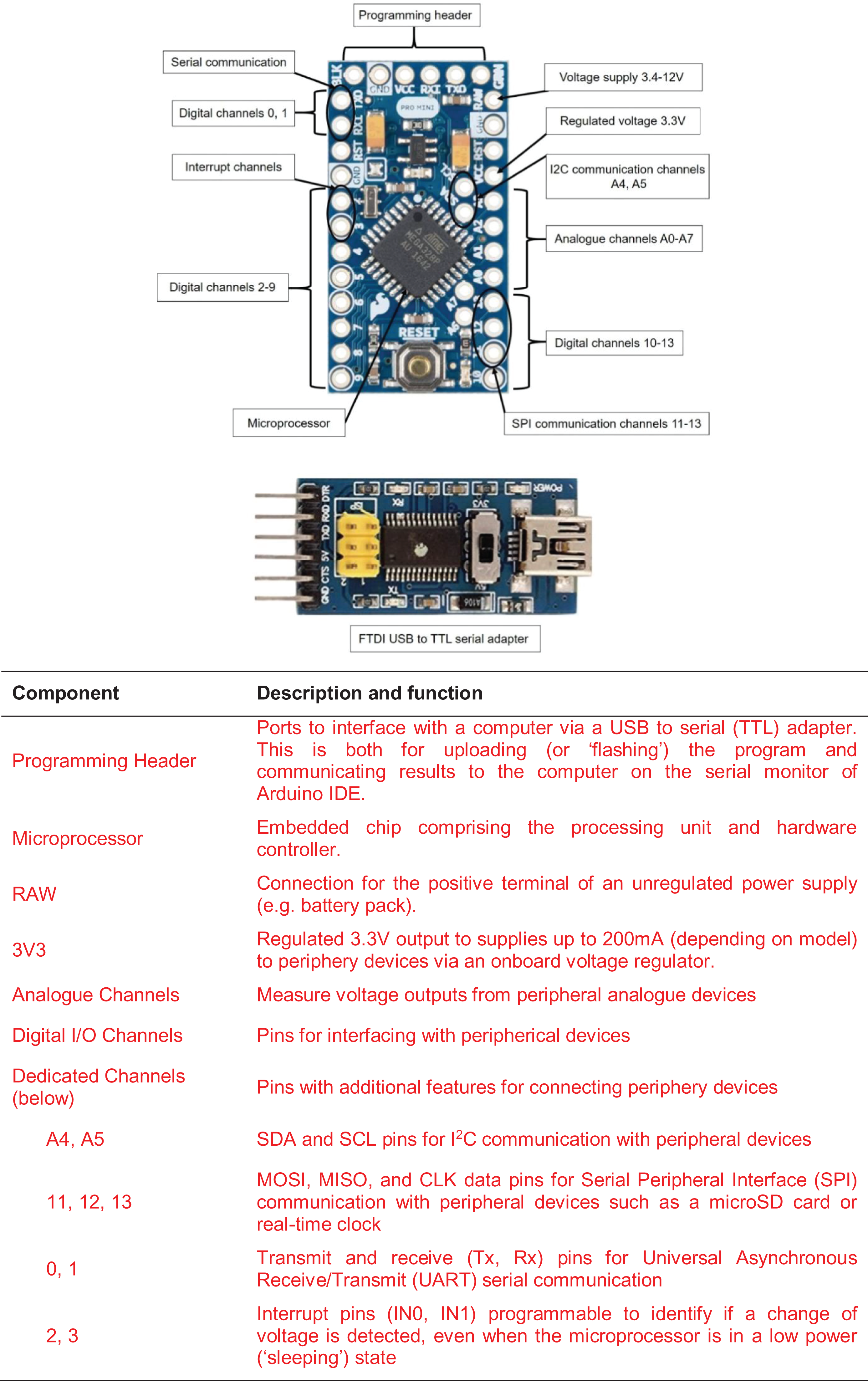
Pro Mini anatomy, detailing the components and port functions common to many microcontrollers. Note: port numbers are specific to the ATmega328P microprocessor.
Though the development of microcontrollers started many years prior to the emergence of Arduino (notable precursors include PIC and Parallax microcontrollers), the development of Wiring and Arduino was pivotal in transferring microcontroller programming from the hands of specialised engineers to wider audiences. Prior to Arduino, most microcontroller prototyping tools were prohibitively expensive and required steep learning curves (D’Ausilio, 2012; Kusher, 2011). Under the supervision of professors from the Interaction Design Institute Ivrea, Wiring (the predecessor of the Arduino programming language) was developed as a simplified coding language for programming Atmel microprocessors. Thus, the combination of the simplified, OSS (the Arduino Integrated Development Environment – hereafter, Arduino IDE) and widespread availability of low-cost hardware (Arduino boards – based on Atmel’s ATmega processors – in addition to other OSH microcontrollers programmed through the Arduino IDE, for example, the Adafruit Feather, ESP8266, RedBear and Particle Photons or Electrons) led to the widespread adoption of microprocessors by hobbyists and the public (Furber, 2017). Through the release of tutorials, troubleshooting forums and continual software and hardware development, the open-source nature of Arduino and other OSH microcontrollers has diminished the learning curve and created a growing user community of beginners and experts. The non-technical and inexpensive characteristics of OSH such as Arduino has also transformed citizen science (research conducted by amateur scientists; Stevens et al., 2014) and presents opportunities for innovative teaching and education (e.g. Giocomassi Luciano et al., 2019; Lim et al., 2020; Plaza et al., 2018).
1.3 Purpose of the paper
This paper aims to catalyse and accelerate the deployment of low-cost sensors for environmental research. It draws on 6 years’ experience developing, testing and deploying a range of Arduino-based, low-cost environmental sensors by staff and students of the Department of Geography at King’s College London (KCL). The impetus for each project varied: some were geared towards research advancements while others were initially developed as teaching activities. In each case, numerous unforeseen challenges have helped us develop smooth, effective workflows and reliable, research-grade data are now rapidly emerging. The following sections explain the core components of an Arduino environmental data logger before presenting six case studies: (a) a water table depth probe; (b) an air quality monitor; (c) an aquatic water quality multiprobe; (d) a customisable multi-parameter weather station; (e) a time-sequencing sediment trap and (d) a sonic anemometer for monitoring wind-blown sand dynamics. Lastly, we highlight frequently encountered pitfalls and outline best practice methods to maximise success rates for researchers new to build-it-yourself hardware construction and programming.
We intend this paper to act as a transformative platform and the key reference for physical geographers (and environmental scientists more broadly) looking to embed low-cost environmental monitoring into their research activities. Full schematics, code, component costs and purchasing guidance to reproduce our designs are available on our KCL Geography Environmental Sensors Github repository (https://github.com/KCLGeography/environmental-monitoring) and FreeStation project website (www.freestation.org). Costs reported in this paper are based on purchases made by the KCL Geography Environmental Sensor group during the 2019/20 financial year. In our view, careful deployment of open-source, low-cost environmental sensors will deliver step-change improvements to global environmental monitoring and management.
II Environmental sensors
2.1 Background to Arduino open-source hardware and software
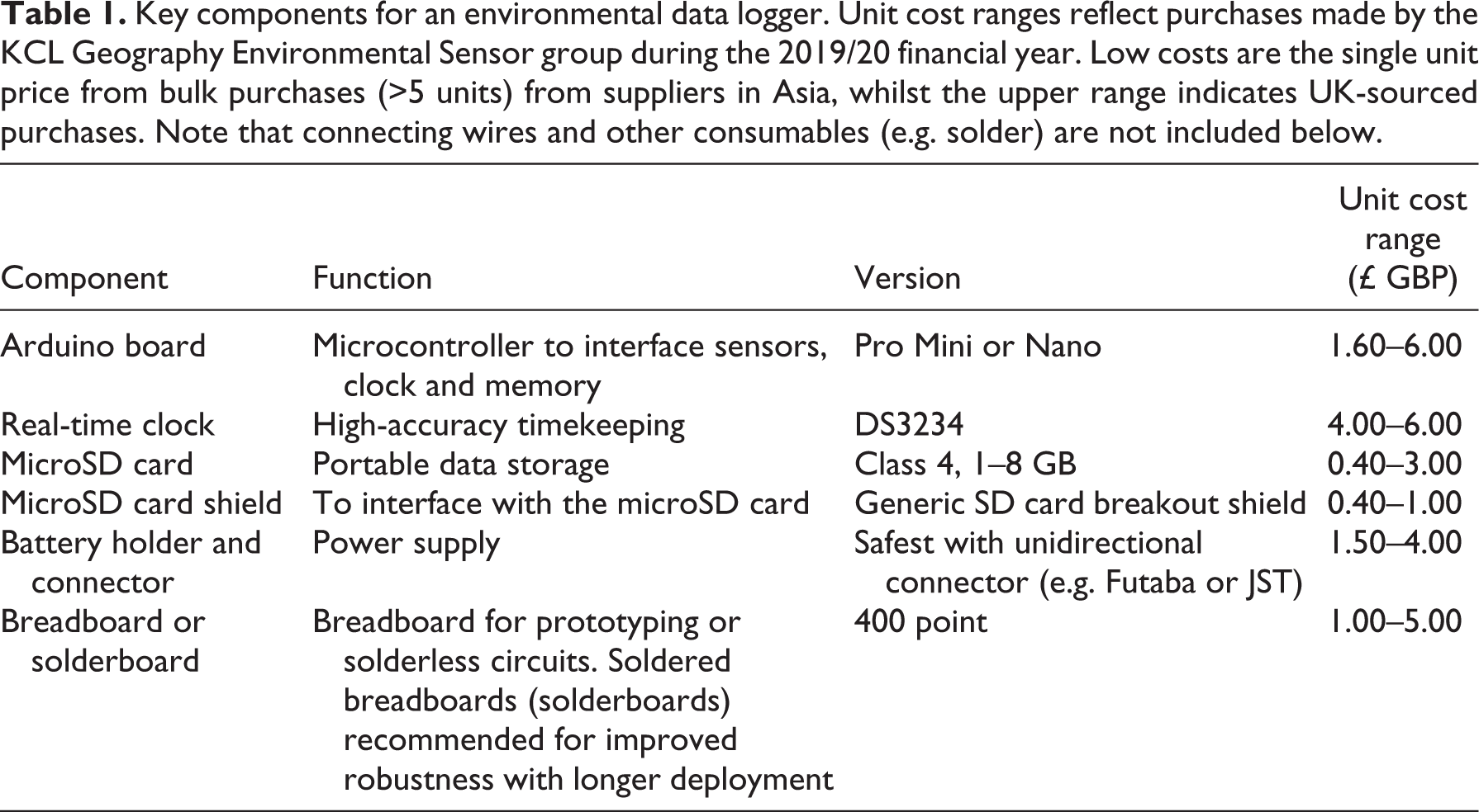
Arduino is a brand of microcontroller boards with their own processor and memory that uses code to control and communicate with electronic devices (Karvinen and Karvinen, 2011). The Arduino programming language is based on C/C++ that is accessed via a user-friendly IDE. An enormous online community provides technical support as well as an extensive list of existing libraries (collections of code that provide bespoke functionality for individual sensors). Despite their versatility, microcontrollers are on their own inadequate for formal scientific environmental monitoring. Core components required for most sensors are described in Table 1. Peripherals such as microSD card shields and real-time clocks can be connected via breadboards and jumper wires (soldered or unsoldered), while bespoke printed circuit boards (PCBs) can be used to simplify construction and minimise connectivity issues such as loose wiring or poor soldering. Components can be easily acquired from UK or overseas sellers. Costs (Table 1) are usually lower from suppliers in China, for example, at the expense of extended delivery times and delays due to customs duties. UK, European or US sources can be an order of magnitude higher.
Key components for an environmental data logger. Unit cost ranges reflect purchases made by the KCL Geography Environmental Sensor group during the 2019/20 financial year. Low costs are the single unit price from bulk purchases (>5 units) from suppliers in Asia, whilst the upper range indicates UK-sourced purchases. Note that connecting wires and other consumables (e.g. solder) are not included below.
2.2 Water table depth probes
Tropical peatlands are one of the most carbon (C) dense ecosystems in the world, storing 3% of global soil carbon on 0.25% of the total land area. Peatlands in Southeast Asia have been widely deforested and degraded over the past few decades, mainly by employing fire and drainage, resulting in their conversion to a net carbon source (Evers et al., 2017). These disturbances result in loss of vegetation structure and enhance peat oxidative decomposition. To assess the impact of land-use change on peatland CO2 emissions (e.g. through gas chamber experiments), flux measurements must be supplemented with water table and soil temperature monitoring. An ongoing CO2 and CH4 flux monitoring site in the tropical peatlands of Belait District, Brunei, consists of 10 sampling sites with bored water table monitoring wells. Conventional water depth sensors (e.g. Van Essen Diver) are relatively expensive at approximately £600 (GBP) per unit (Table 2). To boost monitoring capacity, our group developed a low-cost water table depth sensor (∼£40) that can be easily integrated with water and/or soil temperature sensors.
Cost and accuracy comparisons between two commercial water depth loggers and the second iteration of the low-cost sensor used in this case study. Operating conditions and technical specifications are those reported on manufacturer datasheets. Unit costs are accurate as of April 2020.
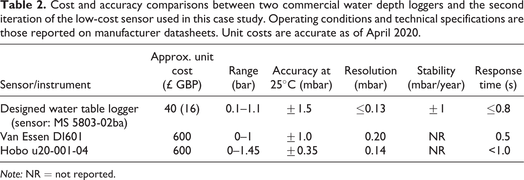
Note: NR = not reported.
Our first model combined a differential pressure sensor (NXP MPX5010DP) with an analogue-to-digital converter (ADC) and the standard Arduino logging components outlined in Table 1, housed inside a weatherproof junction box. The differential pressure sensor has two tube connections: one is submerged in the well, sensing water head pressure and atmospheric pressure, and the other is exposed to atmospheric pressure only. There were a number of advantages to this setup: only the tube needed to be submerged so all electronics were housed above ground; the differential nature of the measurement provides high-precision data; and there is no need for separate measurements of atmospheric pressure. The major disadvantage was that leaving the above-ground tube exposed for atmospheric pressure measurements made it overly susceptible to humidity and insects, resulting in failure or heavy degradation of all units.
Our second, more successful approach used a single pressure sensor (TE Connectivity MS5803-02ba). Here we use a 2-bar sensor (up to ∼10 m water depth; variants of the MS5803 module are available for either deeper, or better precision for shallower, deployments). The sensor and Arduino components are housed inside a waterproof aluminium tube (Figure 2) with screw-threaded caps at each end, which sits inside the well. The space constraints of the tube necessitated direct-soldering of short wires onto components and the small lithium ion battery (there was insufficient space for a battery holder). This approach meant atmospheric pressure had to be measured separately and assembly was more challenging. The sensor is delicate and must be directly exposed to water pressure while electronic connections are kept waterproof. Our solution was to attach a small segment of rubber tubing to the protruding pressure sensor; this tubing was fed through a drilled hole in one end of the tube housing. An epoxy coating was applied to the tube cap, fixing the sensor and rubber tubing in place and isolating the exposed sensor from the Arduino microprocessor and core peripherals. Exposed connections required taping to minimise the risk of electrical shorting, and fitting the direct-soldered wires into the tube also introduced a risk of ripped wires. Thread seal tape was used on the screw threads for the housing to ensure waterproofing.
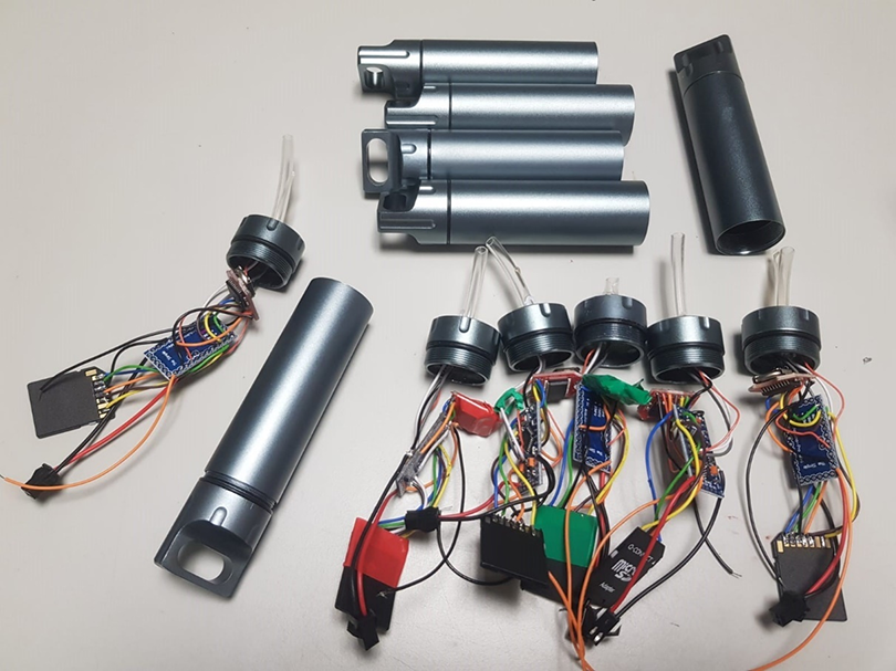
A set of water table depth loggers designed following the second, more successful approach using a single pressure sensor (Note: Li-ion battery not yet connected). See text for details.
An Arduino-based pressure sensor was deployed alongside a Van Essen Diver for a 2-month period at one of the 10 wells in Brunei. Sensor performance was assessed by coefficient of determination (r2 ), root mean square error (RMSE; cm), mean absolute error – a good measure of average performance – and mean bias error (MBE), which provides a useful evaluation of bias dimension (Figure 3; Table 3; Concas et al., 2020). As a further test, data presented in Figure 3 have not been corrected for atmospheric pressure or water temperature (how comparative commercial sensors also function). The Arduino-based sensor captured diurnal variations in pressure as well as warming and cooling of the water column to a high degree of sensitivity, but with a systematic offset of 262 cm. After applying the linear calibration, the Arduino-based sensor showed marginal bias (MBE = –7.11%) and a low RMSE of 1.88 cm, well within the necessary accuracy for peat GHG flux estimates (Lupascu et al., 2020) or multi-year water table monitoring (Mew et al., 1997).
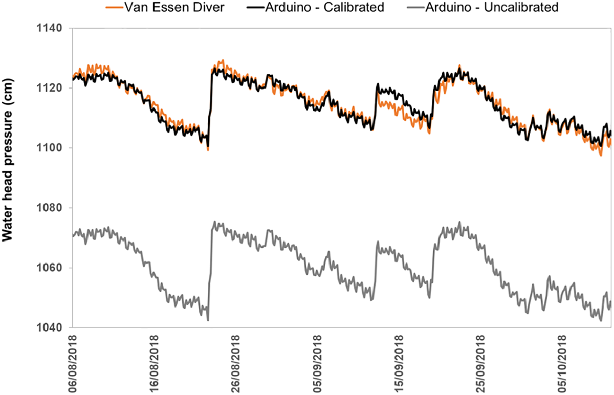
Comparison of water head pressure measured by the Arduino-based sensor (£16; grey and black lines) and a commercial Van Essen Diver (£600; orange line). The Arduino sensor shows strong performance (black line; RMSE = 1.88 cm; Table 3) after applying a linear calibration (y = 0.7873x + 280) to the raw measurements (grey line). Both loggers were deployed in the same well for 2 months. Values have not been corrected for atmospheric pressure or water temperature.
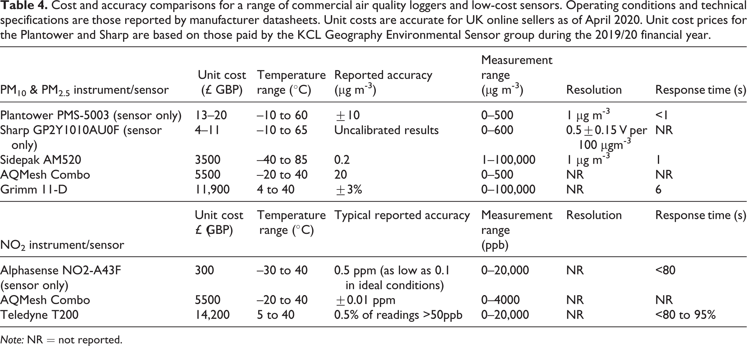
Assessment of Arduino-based sensor performance against the commercial Van Essen Diver using data from a 2-month deployment in a peatland monitoring well in Brunei. These estimates use the calibrated measurements (see Figure 3).
Note: r 2 = coefficient of determination; RMSE = root mean square error; MAE = mean absolute error; MBE = mean bias error.
2.3 Air quality loggers
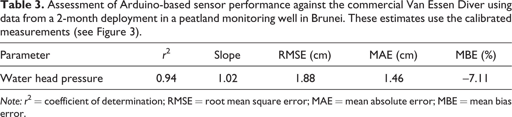
The pervasive threat of poor air quality in urban settings and its acute physiological effects are becoming clear (Atkinson et al., 2016; Kelly and Fussell, 2019; Sundell et al., 2011). Gaseous and particulate emissions have been linked to greater risk of child obesity (Kim et al., 2018), adverse effects on foetal growth (Smith et al., 2017), decreased educational performance (Mendell et al., 2013; Wargocki et al., 2020) and more frequent incidences of dementia in London (Carey et al., 2018), for example. In urban areas, the particulate component is predominantly derived from vehicles through combustion emission, braking and tyre abrasion as well as domestic wood burners, while the gaseous fraction is primarily released during fossil fuel combustion (Vicente et al., 2015). Urban air quality is typically monitored using fixed, ground-based stations. Costs of such configurations run to many thousands of pounds per instrument (Mead et al., 2013) and stationary infrastructure is less suitable for pinpointing emission point-sources and assessing personal exposure and localised risks. Low-cost air pollution sensors offer valuable granularity and portability with initial studies showing promise (Bulot et al., 2019; Mead et al., 2013; Munir et al., 2019; Piedrahita et al., 2014). We have developed Arduino-based sensors to measure particulate matter (PM1, PM2.5 and PM10) and trace gases (NO2, O3 and NO) for ∼£410, which show good performance when tested against the London Air Quality Network (LAQN).
For particulate matter, we determined the most effective sensor to be the Plantower PMS-5003 sensor (Table 4), an optical laser-scattering sensor that achieves high accuracy (98% counting efficiency of PM ≥ 0.5 µm; Plantower, 2016). Its rapid measurement response time (≤10 s) also allows reliable measurements to be made in transit. Tests of cheaper Sharp GP2Y1010AU0F sensors showed inferior performance and the need for continuous calibration – a difficult undertaking for particulate matter requiring equipment in the order of tens of thousands of pounds. Electrochemical gas sensors manufactured by Alphasense have been used to measure NO, NO2 and O3, with reported accuracies below 1, 0.5 and 0.5 ppm, respectively (Alphasense, 2017). We adapted two designs: one incorporates a pump, air flow circuitry and filter system that keeps separate the PMS-5003 inlet and outlet before removing particulates prior to entering the gas chamber (Figure 4). The second, simpler configuration fixes the particulate matter and gas sensor inlets and outlets to separate holes drilled through the housing (Figure 5). The Alphasense sensor output is between 300 and 400 mV so a 16-bit ADC was used (the ADS1115 module), which has far superior voltage range and resolution compared to ATmega328P’s 10-bit ADC (65,536 individual detectable levels compared to 1024 respectively). We also ensured sampling intervals were programmed to mimic the instrument’s inhalation and exhalation cycle. We usually mount a Bosch BME280 that measures temperature, relative humidity and barometric pressure or a BME680 (which also samples volatile organic compounds) alongside the PMS-5003.
Cost and accuracy comparisons for a range of commercial air quality loggers and low-cost sensors. Operating conditions and technical specifications are those reported by manufacturer datasheets. Unit costs are accurate for UK online sellers as of April 2020. Unit cost prices for the Plantower and Sharp are based on those paid by the KCL Geography Environmental Sensor group during the 2019/20 financial year.
Note: NR = not reported.
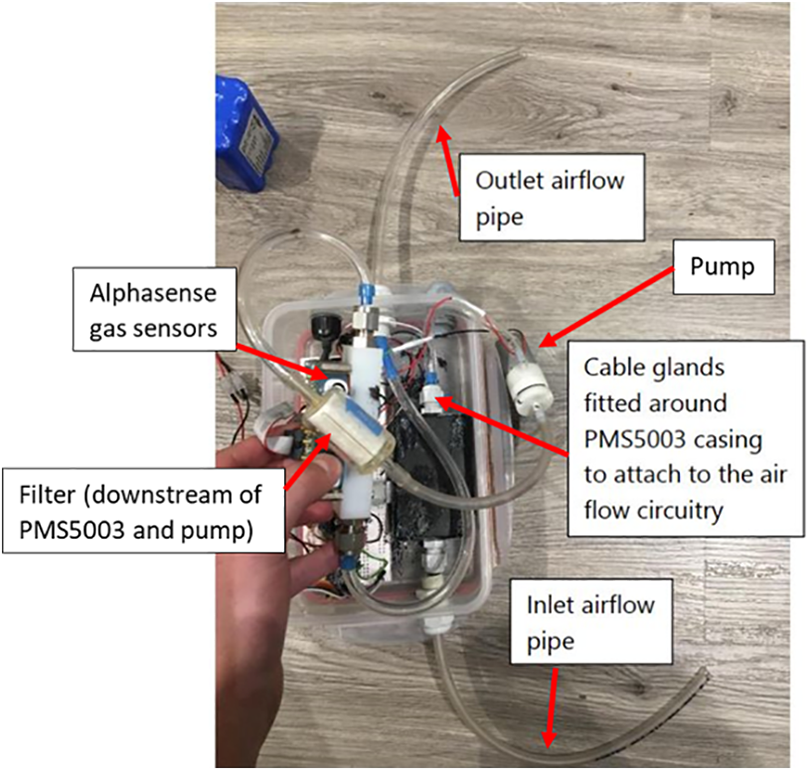
Air quality sensor array comprising a Plantower PMS5003 and a set of Alphasense gas sensors. This configuration encompasses a EPA filter and pump for particularly dusty environments, or where faster reading stabilisation is required (e.g. handheld applications).
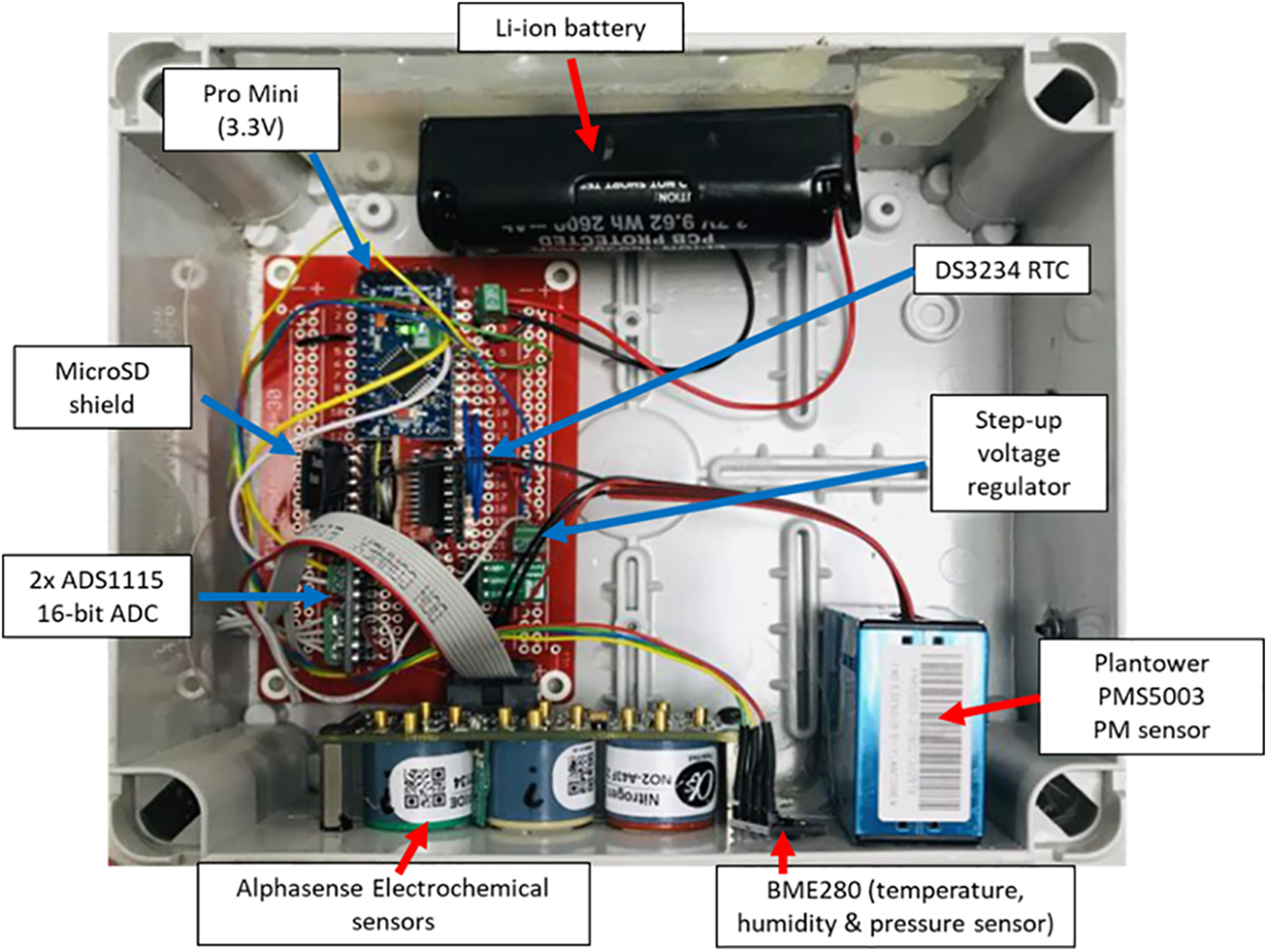
Air quality sensor array comprising a Plantower PMS-5003 and a set of Alphasense chemical gas sensors. This second design is simpler but assumes deployment at a fixed location.
We assessed the performance of the Arduino-based air quality sensors against the LAQN flagship kerbside monitoring station on Marylebone Road, a major arterial route through west London. Our sensors were positioned on its roof (2 m above ground level) for 5 days in February 2018. The Marylebone LAQN station measures PM2.5 on a Filter Dynamics Measurement System and NO2 via chemiluminescence. The Plantower PMS3005 and Alphasense NO2-A42F showed strong performance overall (Figure 6, Table 5). Our sensor returned higher maximum PM2.5 readings and the RMSE indicated the low-cost sensors appeared to be marginally oversensitive when measuring the highest concentrations of PM2.5, with the exception of an over-estimated peak in PM2.5 on 4 February. Mean concentrations were similar for PM2.5 and NO2 and the low MBE (Table 5) indicated limited systematic over- or underestimation, however. Importantly, the low-cost sensors accurately captured the temporal picture, including rush-hour peaks and variation between weekday and weekend traffic density (Figure 6).
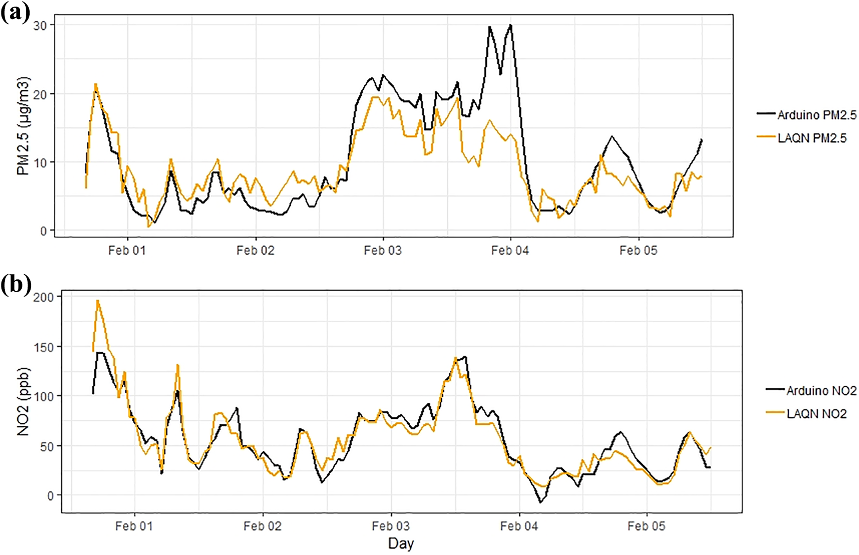
Data comparison of (a) PM2.5 and (b) NO2 measurements made by an Arduino-based sensor (black lines) and the London Air Quality Network’s Marylebone monitoring station over a 5-day period in February 2018. The Arduino-based sensor sits on top of the station to ensure measurements are made at similar heights.
Assessment of low-cost sensor performance based on a 5-day deployment at the LAQN flagship Marylebone monitoring station.
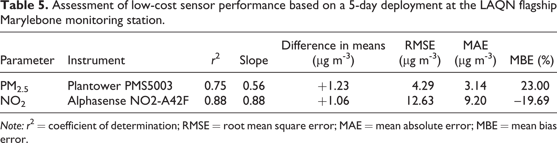
Note: r 2 = coefficient of determination; RMSE = root mean square error; MAE = mean absolute error; MBE = mean bias error.
The growing commercial market for personal air quality monitors has raised concerns about data quality (Lewis and Edwards, 2016). Our bias estimates compare favourably to performance testing of a Plantower PMS5003 by Bulot et al. (2019; RMSE for PM2.5 of 6.5–7 µg m-3) and Sayahi et al. (2019; RMSE for PM2.5 of 5.5–9.6 µg m-3). Although other researchers (e.g. Feenstra et al., 2019; Johnson et al., 2018) report mixed performance between different models of low-cost air quality sensor. There are numerous models for measuring a specific environmental parameter (e.g. airborne particulate concentration) on the market; these should evidently not be clumped into a homogenous class of ‘low-cost sensors’. The Plantower performs well in most studies although Kelly et al. (2017) showed deterioration in accuracy when particulate concentrations exceeded 40 µg m-3. This underscores the importance of recognising sensor choice should be guided by deployment setting coupled with comprehensive field testing and sensor-specific calibration. Meteorological factors, especially temperature and relative humidity, can also have large effects on sensor readings (e.g. Feenstra et al. 2019; Jayaratne et al., 2018). We posit that build-it-yourself sensors can help overcome such limitations by increasing capacity for paired deployments of air quality and meteorological sensors rather than depending on, for example, regional weather station data (e.g. Bulot et al., 2019).
Our sensors produce promising research-grade data and are enabling important research questions to be explored at the individual or community level. For example, one deployment showed the installation of an ivy green screen at a primary school in central London decreased NO2 concentrations during peak traffic congestion by 35%, whilst another confirmed that choosing an optimal form of public transport to minimise personal exposure in London presents a predicament: particulate matter was higher when walking, cycling, or on the Underground, but time inside buses and cabs increased exposure to NOX.
2.4 Water quality loggers
Threats to water quality and aquatic biodiversity from human activities are a global issue. Despite widespread acknowledgement that pollution is a major threat to the sustainable management of aquatic environments (Rockström et al., 2014; Vorosmarty et al., 2010), local- and regional-scale initiatives are constrained by the limited availability of real-time, on-the-ground data (Behmel et al., 2016). Alongside warnings of ‘data-rich but information-poor’ scenarios around water quality monitoring networks (Ward et al., 1986), the temporal and spatial scale of water quality testing is largely determined by finance and logistics, particularly due to the expense of commercially available monitoring systems. Here we present our efforts to develop an Arduino-based multi-parameter probe for water quality monitoring.
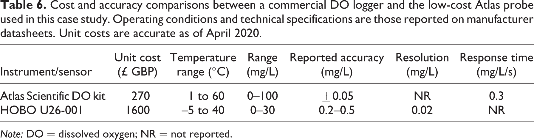
Following global monitoring efforts (World Health Organization [WHO], 1996; WHO, 2004), we chose to focus on temperature, conductivity, and DO due to overall cost and likelihood of producing accurate readings (Wagner et al., 2006). Temperature influences most water quality parameters (WHO, 1996). Not only do temperatures in water bodies vary over 24 h, but their daily averages change throughout the year (Brümmer et al., 2003). DO, an indicator of aquatic biological health, is related to the photosynthetic and metabolic activity of aquatic organisms. Given DO is affected by temperature and there are noticeable diurnal and seasonal variations, temperature and DO are monitored simultaneously (Kannel et al., 2007). We chose the Atlas Scientific DO kit, as galvanic cell-type sensors have short response times and appropriate robustness for outdoor deployments (Wei et al., 2019) at a cost of £270 (Atlas Scientific, 2019; Table 6). The associated shield allowed more straightforward calibration and programming because it directly calculates actual DO values from the voltage reading. Conductivity is a commonly measured water quality parameter (Wagner et al., 2006) and long-term monitoring can be useful for tracking pollution sources (Morrison et al., 2001). We used the DFRobot electrical conductivity probe and shield (£60) to achieve an optimal balance between cost and accuracy. The glass design protects the sensitive electrode, providing additional durability (DFRobot, 2017).
Cost and accuracy comparisons between a commercial DO logger and the low-cost Atlas probe used in this case study. Operating conditions and technical specifications are those reported on manufacturer datasheets. Unit costs are accurate as of April 2020.
Note: DO = dissolved oxygen; NR = not reported.
The River Brent in London (UK) has a long history of poor water quality, and river restoration efforts are ongoing (Thames21, 2019). We deployed Arduino-based loggers (Figure 7) in two locations along the River Brent – a river restoration and an unrestored site – for 1 week in February 2018 (Lavelle et al., 2019). We also deployed a commercial logger (HOBO U26-001) measuring temperature and DO at the unrestored site to facilitate performance evaluation. All loggers were placed in the middle of the river on wooden stakes, hammered 15-cm deep into the riverbed and protected with rocks for security.
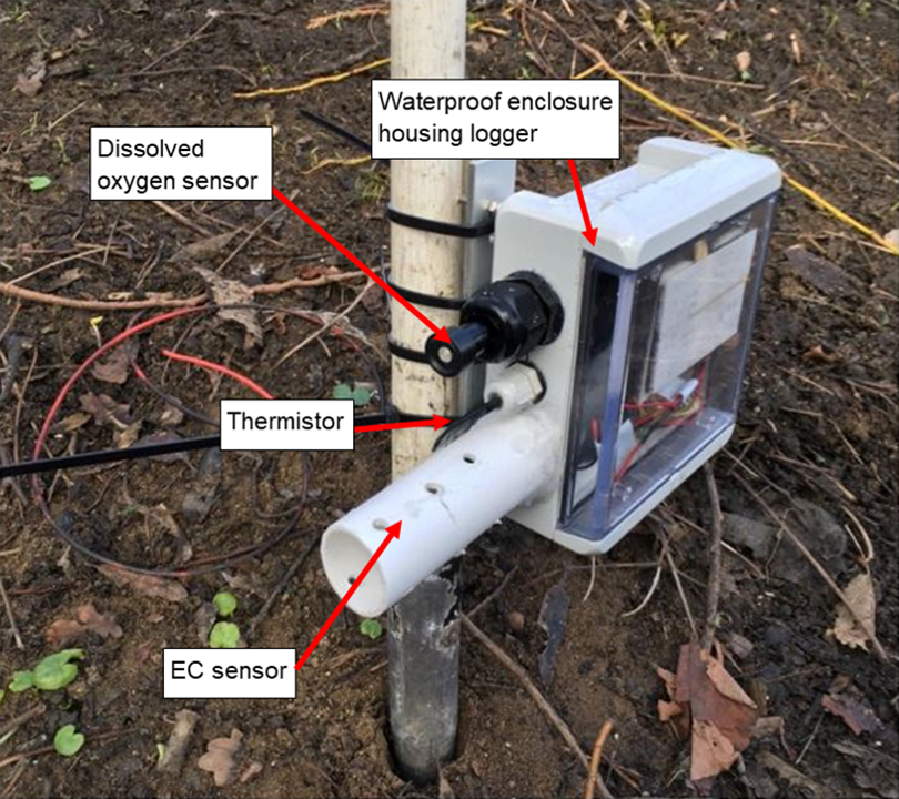
Deployment configuration of the water quality multiprobe.
The Arduino-based DO and temperature time-series closely follow diurnal fluctuations as measured by the Hobo logger (Figure 8). Temperature was measured particularly effectively (r2 = 0.97, RSME = 0.29°C; Table 7). In situ DO measurements showed satisfactory correlation with the Hobo logger (r2 = 0.87) but an offset is evident, with the Hobo logger giving readings ∼20% higher. Individual sensor calibration of the thermistors was straightforward but acquiring accurate DO readings was more complicated. It is difficult to determine whether the lower mean readings are associated with the inbuilt Atlas Scientific calibration, electrical interference introduced by sensor integration or issues with the data transfer (Siragusa and Galton, 2000). Nevertheless, applying a post-deployment linear calibration function leads to excellent accuracy, with an MBE well below 1% (Figure 8; Table 7). Arduino-based DO sensors should produce reliable readings provided an initial site-specific calibration is performed. Conductivity measurements were consistently divergent, leading us to suspect issues with probe accuracy. Data are not reported here and difficulties with conductivity probe calibration persist despite extensive lab testing.
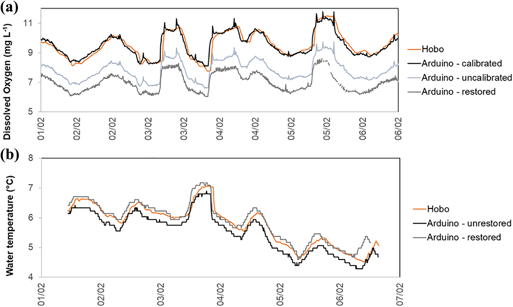
Comparison of (a) dissolved oxygen and (b) water temperature measurements at the unrestored and restored sites. Data were measured 01–06 February 2018 by an Arduino-based sensor (£380; black and grey lines) at both sites and a HOBO U26-001 (£1,600; orange lines) at the unrestored site to evaluate performance. The Arduino-based DO sensor deployed at the unrestored site shows strong performance (black line; RMSE = 0.31 mg L-1; Table 7) after applying a linear calibration (y = 1.184x + 0.256) to the raw measurements (light grey line).
Assessment of Arduino-based sensor performance against the commercial HOBO U26-001 using data from a 7-day deployment in an urban stream in London, UK. These estimates use the calibrated measurements (see Figure 3).
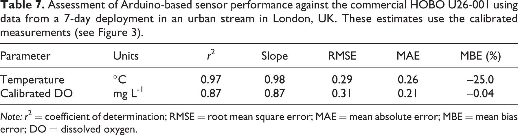
Note: r 2 = coefficient of determination; RMSE = root mean square error; MAE = mean absolute error; MBE = mean bias error; DO = dissolved oxygen.
A major pitfall in the construction of these probes was underestimating the time requirements for troubleshooting. Non-compatibility between sensors, especially during attempts to eliminate electrical interference, was an unexpected but major technical challenge. Achieving a watertight enclosure was a foreseeable challenge but producing a design using ‘low-cost’ materials with adequate ruggedness for aquatic deployment was enormously time-consuming. The number of prototype probes gives some insight into the time commitment. Four models were iteratively produced, each the result of six documented field tests and numerous laboratory trials. We have developed two fully functional multiprobes but five others were tested and failed due to calibration inaccuracy, water intrusion, faulty parts or short-circuiting. Repeated replacement of parts and calibration chemicals is a hidden labour and financial cost.
Reproducing our functional model does represent an economically competitive alternative to commercial equipment, with scope for further improvements to the external housing. One of the most exciting aspects is that the technology allows for multiprobes to be customised for specific studies, such as the inclusion of nitrogen, phosphorous, nitrate, colour or chlorophyll sensors to monitor eutrophication in freshwater systems (Ferreira et al., 2013). In situ water quality monitoring is complicated because a complete and precise assessment cannot be reached unless several interacting parameters are measured simultaneously. While careful calibration will be required for each sensor added to a multiprobe, low-cost, continuous water quality loggers offer a valuable method for broadening the density of routine monitoring. These networks could go a long way to establishing long-term records of baseline conditions and identifying specific environmental pollution sources.
2.5 Automated weather stations
Meteorological data are fundamental to climatic, hydrological, ecological and geomorphological research. Multivariable weather stations are the standard system for monitoring meteorology, with >47,000 locations globally officially recording precipitation and >24,000 recording mean monthly temperature (Hijmans et al., 2005), though many more unofficial (amateur) weather stations now exist. A weather station normally measures air temperature, atmospheric humidity and pressure, precipitation, solar radiation, and wind speed and direction. These variables allow an assessment of surface energy, water balances and horizontal fluxes of air. Automatic weather stations can measure sub-hourly but usually aggregate data to hourly or daily averages or totals. The cost of commercial weathers stations increases with the number of measurable variables (Table 8). Multivariate stations can be priced in the thousands of pounds before specialist installation and maintenance is factored in.
Cost and accuracy comparisons between two commercial weather sensors and the low-cost Bosch BME280 used in several of our case studies. Operating conditions and technical specifications are those reported on manufacturer datasheets. Unit costs are accurate as of April 2020.
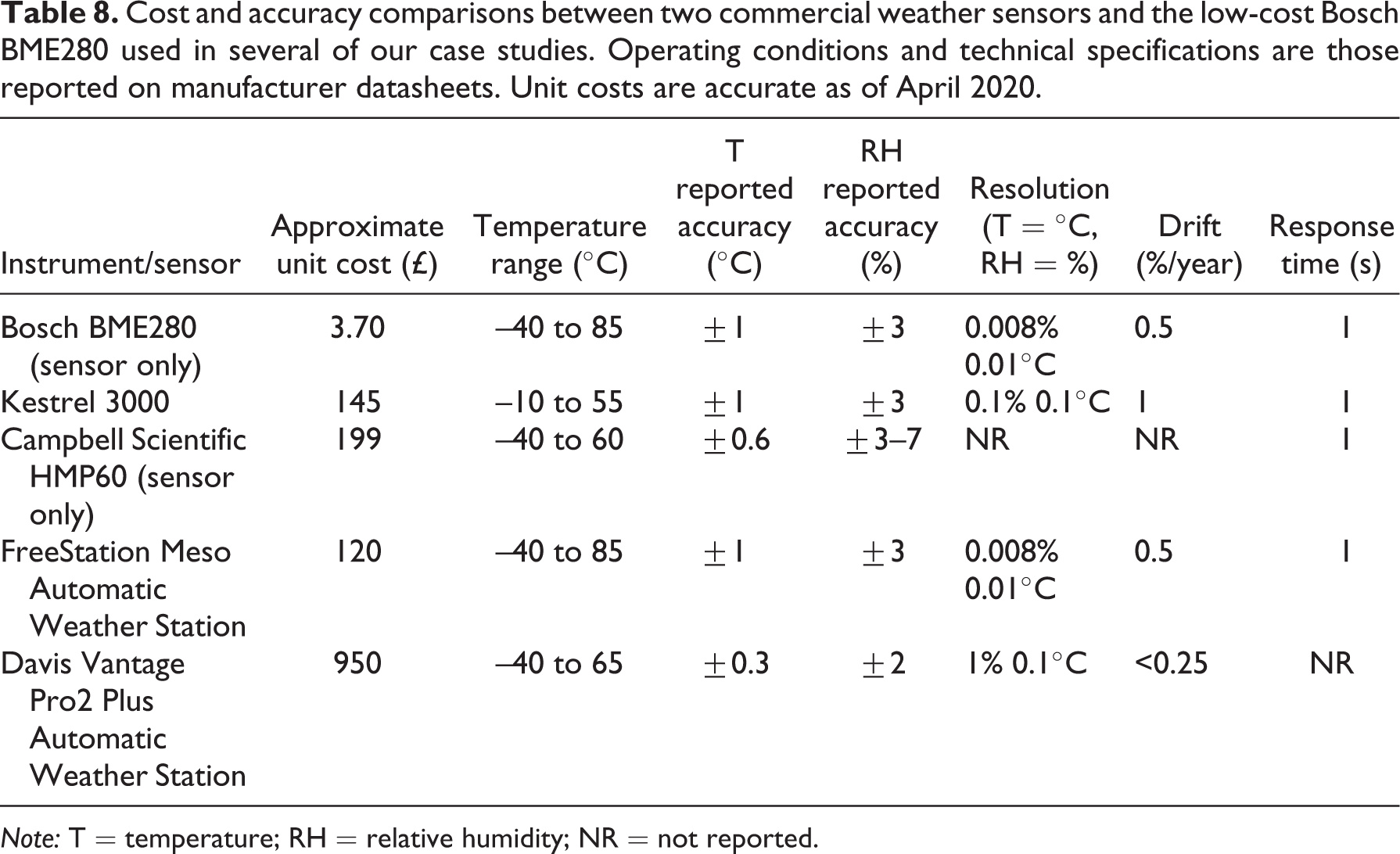
Note: T = temperature; RH = relative humidity; NR = not reported.
Grid-connected weather stations are particularly sparse in low-income countries and their state of maintenance can be poor (WMO, 2019). Climate change is likely to have disproportionately large impacts in these regions so longitudinal data collection at local scales is critical. The FreeStation project (http://www.freestation.org/) is working to redress this issue by expanding meteorological monitoring capacity using open-source and low-cost instrumentation. Since 2014, FreeStation has developed open-source designs for a range of low-cost instrumentation and loggers. These include standalone and web-connected automatic weather stations (AWS) based on Arduino and Particle microprocessors. FreeStation AWS have a component cost 3–13% the cost of a commercial station and require 2–4 h of unskilled labour to build using the detailed build instructions at www.freestation.org/building. The stations are designed to be easily built from accessible components as well as accurate, robust and easy to transport and install. The FreeStation Meso station includes precipitation, temperature, humidity, pressure, wind speed and direction and solar radiation (Figure 9(a)). It reads instruments every 10 min and writes hourly summaries to an on-board microSD card. The Meso can use an Arduino Pro Mini, a Particle Photon, or RedBear microprocessor. The MesoLive (Figure 9(b)) has the same instrumentation on a smaller footprint with cellular connectivity and access to data via a simple web application programming interface (API). More than 219 stations are currently collecting data at 43 sites in 15 countries and the design has evolved significantly over time, guided by deployments in a range of environments. FreeStations are currently in use by research projects in deserts, temperate and tropical forests as well as by schools, NGOs and some governmental authorities.
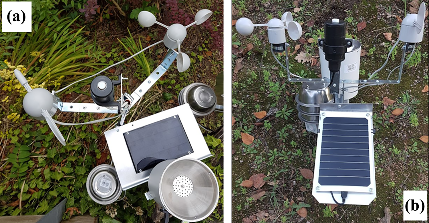
(a) The FreeStation Meso Automatic Weather Station (AWS) and (b) the FreeStation MesoLive AWS.
As our most established research programme (since 2014), FreeStation sheds valuable light on long-term sensor robustness and performance. Promisingly, there have been zero sensor failures in field deployment. Occasional data loss has occurred due to faulty SD cards, loss of power or external interference from animals (rabbits in the UK; crocodiles in Burkina Faso!) or extreme weather. This shows comparable or superior performance to commercial data loggers, which report failure rates of 7–27% (Mickley et al., 2018). Moreover, failure in a commercial device is usually permanent because they are shipped as a sealed product. This means one faulty internal part can render the device inoperable, whereas individual components can be easily and cheaply replaced in low-cost designs. This is an enormous benefit for the unimpeded collection of long-term time-series data. This also minimises issues around sensor drift, for example. We have observed sensor degradation in very humid environments, such as cloud forests, but swapping the meteorological sensors on an annual or semi-annual basis has avoided this issue.
FreeStations are built around the FreeStation PCBs and FreeStation firmware, which allow ‘plug and play’ connectivity of a variety of sensors through standard RJ45 and RJ12 cables (commonly known as ethernet and phone cables). FreeStations are designed to be buildable by students without prior electronics knowledge or interest in microprocessors, and we work with students, extension workers and government technicians to develop local capacity. Shipping build materials and components overseas has been a challenge, however. Most FreeStation components are sourced from the web and direct postage has been problematic, with lengthy delays at customs. Bringing parts and stations from the UK as personal baggage during research visits is easier but is not a long-term option. The power and programmable memory of the Arduino platform has also imposed technical constraints on integrating multiple meteorological sensors and managing the data streams emerging from multiple deployments. Data streams are managed through a web platform and API (Figure 10), which is capable of quality control, combining incoming data streams with forecasts, early warning and direct connection to web-based modelling and policy support tools such as WaterWorld and Eco: Actuary (www.policysupport.org). This kind of integration of real-time data streams with web-based models has significant potential in environmental forecasting and management.
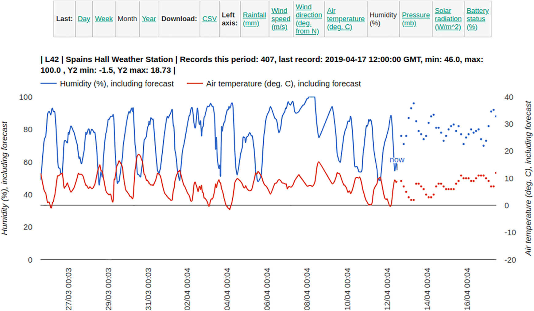
An example of the live data stream from a UK FreeStation weather station, including forecast data (FreeStation, 2019).
The FreeStation project has now moved beyond weather monitoring. As part of the Pathways out of Poverty for Reservoir-dependent Communities in Burkina Faso (POP-BF) project (www.sites.google.com/view/pop-bf), for example, a range of FreeStations have been installed that monitor local weather, water levels in reservoirs using sonar, and soil moisture. These stations are connected to the WaterWorld policy support system to deliver nowcasts and short-term forecasts (communicated via on-board switches and lights) on reservoir volume and soil moisture to advise irrigation and harvest planning. The simplicity of the technology and output has created a locally owned reservoir monitoring system that will continue beyond the lifetime of the project.
2.6 Time-sequencing lake sediment traps
Sediment traps installed in lakes capture particles settling through the water column. Long-term, high-frequency monitoring offers insight into the biogeochemical functioning, sedimentation regime and seasonal changes in biodiversity that cannot be replicated in laboratory experiments (Bonk et al., 2015; Chmiel et al., 2016; Schillereff et al., 2016). Static trap deployment is common but requires manual retrieval, severely restricting sampling frequency, especially at remote sites. Time-sequenced instruments that open separate containers at preprogrammed intervals provide valuable temporal resolution. Commercial versions are costly (>£10,000). Build-it-yourself designs exist (e.g. Muzzi and Eadie, 2002) but require greater expertise in mechanical and electrical engineering. A reliable, low-cost sequencing sampler will therefore transform limnological research, especially in light of funding pressures on long-term lake monitoring programmes. In total, our current design comes to £80.
Initially an undergraduate project, we swiftly appreciated the research potential of an Arduino-based sequencing sediment trap. Our original design comprised three main components: (a) two 3D-printed carousels (d = 187 mm) holding twelve 60 mL NalgeneTM polyethylene bottles, fixed by threaded rod to a stepper motor (Figure 11(a)); (b) cylindrical PVC downpiping that feeds a funnel sitting over the carousel hole (d = 33 mm); and (c) an IP68-rated enclosure housing the stepper motor and Arduino-based electronics. Bottle lids were fixed in carousel holes with epoxy resin and holes bored equivalent to the funnel diameter.
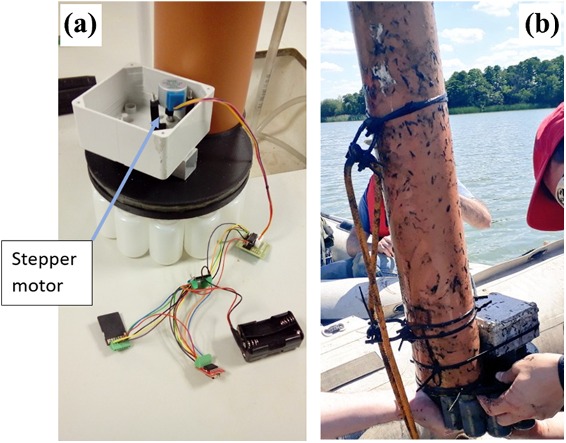
(a) Internal hardware components and (b) post-deployment, highlighting concerns around biofouling. An improved version will incorporate an enclosure around the rotating carousel.
The downpipe (h = 75 cm, outer diameter = 110 mm) aspect ratio of 6.8:1 follows the recommendations of Bloesch and Burns (1980) to ensure representative sediment capture in small lakes. The unipolar 28BYJ-48 stepper motor is cost-effective (∼£2.50) while offering high-precision rotation at low speeds. Although the stepper motor draws 5V, testing confirmed a 3.3 V Pro Mini provided adequate power for 30-day rotation. Different time-steps are easily programmed for alternative applications.
A 12-month test deployment in Crose Mere, Shropshire (52.86°N, 2.84°W) successfully recovered sediment each month. Trap installation involved fixing the downpipe using D-clasps to 5 mm wire held between a basal 20-kg weight and buoys: one larger suspended below the annual minimum lake level to maintain taut deployment and a small, coloured float at the surface. The design was operationally effective but water seepage into the housing was a concern, most likely through the cable gland during axle rotation. Our second version uses shaft seals to minimise water ingress and we are trialling open-source underwater remotely operated vehicle tricks of filling the housing with wax. Trap recovery highlighted two further issues that are easily rectified by using improved enclosures: biofouling (Figure 11(b)) and abrasion of bottle labels. The volumes of trapped sediment dispelled concerns that 60 mL containers are too small, at least in eutrophic, productive lakes.
2.7 High-frequency measurement of wind-blown sand
Research on sand transport by wind includes a rich variety of electronic sensors for measuring and recording physical processes and flows at relatively high frequencies (Hugenholtz and Barchyn, 2011; Sherman et al., 2013). Typical field instrumentation includes sonic anemometers for recording wind vectors, electronically weighing sand traps, sand-grain impact sensors, and laser interference instruments for detecting saltating sand transport rates, and additional equipment such as continuous soil-moisture probes and further meteorological sensors. The acquisition and data storage of high-frequency time series of wind and sand transport measurements are crucial to investigating the relationship between turbulence in the airflow and the spatio-temporal variability of sand transport, displayed particularly by the ubiquitous presence of streamers (also known as sand snakes) in wind-blown sand (Baas, 2008; Baas and Sherman, 2005). Sensors are positioned in close proximity to each other but data outputs of different types are required to be stored synchronously as well as at the original high measurement frequencies. This poses significant challenges to traditional data loggers but provides opportunities for the custom-built and low-cost Arduino-based data acquisition system (DAS).
Our latest research combines sonic anemometry with laser-counter sensors, which have been integrated with an Arduino-based logger system. A Gill R3-50 sonic anemometer provides 3D wind vector measurements at 50 Hz, output via an RS232 serial ASCII data stream, while a Wenglor laser-counter detects sand grains flying through a narrow laser beam, outputting a 100 µs voltage pulse for each interruption (Davidson-Arnott et al., 2009). Traditional dataloggers struggle with these data output and recording requirements; simple and low-cost loggers exist for pulse signals, but typically do not possess RS232 input capabilities and are often restricted in temporal resolution to logging at 1 Hz or less. High-end dataloggers (e.g. Campbell Scientific CR1000X at ∼£1550) on the other hand can handle RS232 input, but have only a few dedicated pulse counter input channels and can be cumbersome to transport. Our Arduino-based solution (∼£45) uses a Due microcontroller board, which operates an 84 MHz processor and can accommodate several dozen count channels as well as RS232 input via an RS232-to-TTL (transistor-transistor logic
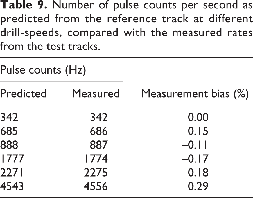
This Arduino-based DAS has been lab tested using a custom-built rotating disc with a series of perforations in its rim, mounted on a multi-speed, belt-pulley driven, bench drill while running the sonic anemometer in front of an ordinary air fan. The purpose of the testing was to verify whether the Arduino-based DAS – the external interrupt routine in particular – was capable of correctly recording the pulses from the Wenglor, even at very high pulse-rates, while also continuously processing the ASCII data stream from the sonic anemometer. The rotating disc had three different tracks of perforations (Figure 12): 72 holes along the rim, 36 holes on the inside track, and a reference track of only four holes covering one disc rotation further toward the centre of the disc.
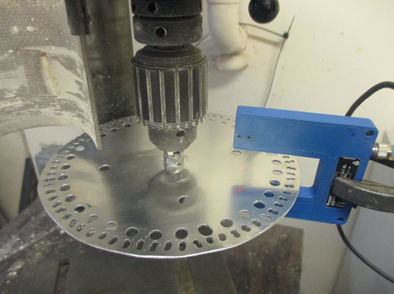
Rotating disc with three perforation tracks, mounted in a multi-speed bench drill, with sideways mounted Wenglor laser-counter fork-sensor (red laser beam reflection visible) used for calibration.
The reference track was used to measure the actual revolutions per minute (RPM)of the bench drill at different speeds (since the nominal spindle speeds from the belt-pulley ratios are not very precise), followed by the two test tracks during the same drill-run. The test results reported in Table 9 show that the number of pulses per second counted on the two test tracks correctly match the predicted number of pulses per second, within the prediction accuracy. During all these tests the ASCII data stream was recorded with no transcription errors. At the highest RPM test, the results show that the system can easily measure and record pulse rates of at least 4500 counts per second (as well as the 3D airflow data) at the required 50 Hz. This exceeds the tested capabilities of commercial logger combinations (Bauer et al., 2018). A pilot field deployment has demonstrated the success and portability of the system (Figure 13) and its compatibility with large-scale particle image velocimetry equipment (Baas and Van den Berg, 2018). The duration for which this DAS can be deployed is only defined by the battery capacity and SD card storage limit, running to several days in the setup used here.
Number of pulse counts per second as predicted from the reference track at different drill-speeds, compared with the measured rates from the test tracks.
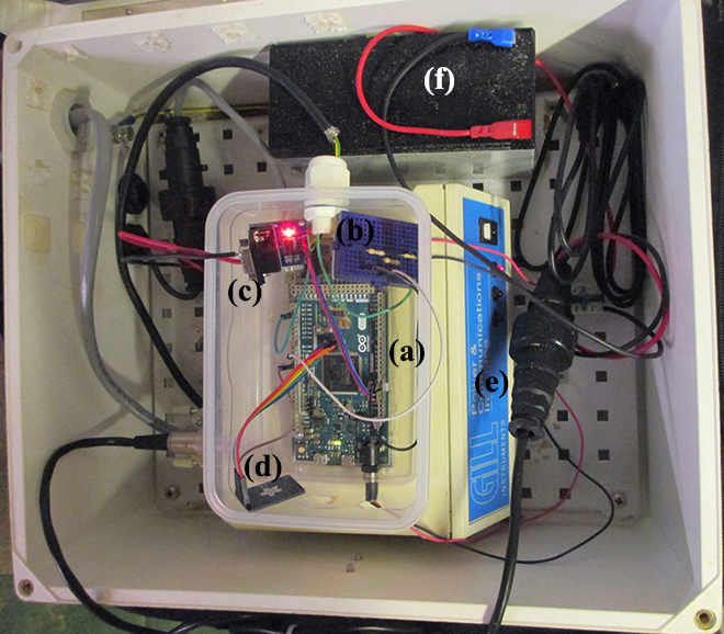
The data acquisition system used for synchronous recording of Gill sonic and Wenglor laser-counter measurements, housed in a portable enclosure. Components: (a) Arduino Due microcontroller board, (b) voltage divider to reduce the ∼11VDC output from the Wenglor to <3VDC input to the microcontroller board, (c) RS232 input from the Gill Sonic communication unit, (d) mini-SD card ‘shield’ for storing the data, (e) Gill sonic communication unit, and (f) 12 VDC battery power supply.
III Common pitfalls, lessons learned and best practice workflow
3.1 Major advances and successes
Our cumulative experience has highlighted the following key considerations from which we have developed a set of best practice guidelines.
3.1.1 Standardised and bespoke circuit boards
While Arduino offers near-limitless adaptability, a key aspect of our streamlined workflow is having core design frameworks. For example, we now have a standard circuit board design for ultra-low-power loggers (important for long-term monitoring) that can be readily adapted to most sensors. Similarly, we have developed replicable methods of incorporating a solar panel onto designs where possible. While we regularly use solderless breadboards for prototyping and as teaching aids, soldered wires are near-essential to minimise the possibility of loose wires and short-circuits. Poor or incorrect wiring is the most common malfunction, in our experience. We are increasingly making use of bespoke PCBs, led by the FreeStation project. Designing PCBs in conjunction with OSHPark is cost-effective, simplifies the electrical assembly and minimises wiring faults while maximising customisability for multi-sensor applications. They can also accommodate web-integrated cellular boards such as the Particle Electron and can be designed to be swapped for the cheaper, Wi-Fi only Particle Photon (https://docs.particle.io/electron/).
For data transfer, the suitability of the standard ADC on board the ATmega328P microcontroller will depend on sensor and research requirements. Our thermistor, conductivity and wind direction sensors all draw 2 V or less. The Alphasense NO2 sensor output, on the other hand, is between 300 and 400 mV so an ADS1115 module was used to improve reading sensitivity, both through focused voltage ranges and 16-bit resolution. This module has far superior resolution (detecting 65,536 voltage ‘steps’ compared to 1024) and voltage range (with a full range as low as ±0.256 V where one step equates to 7.81 pV, compared to 1.08 mV when using the higher resolution 1.1 V reference voltage on the 3.3 V Pro Mini). Our instruments that use digital sensors (temperature and relative humidity modules, DO, Plantower PM sensors, 3D sonic anemometer) have inbuilt ADC convertors and communicate the calibrated readings.
The scope to integrate multiple sensors, each measuring a different environmental parameter, is a major advantage of the build-it-yourself approach but we repeatedly encountered problems of compatibility. This was exacerbated by sensors sourced from new manufacturers that may draw different voltages or conflicting code libraries. The increasing number of clone microcontroller boards on the market may well exacerbate these issues. We therefore use hardware specifically designed for Arduino hardware with pre-existing Arduino libraries for most designs.
3.1.2 Documentation
Developing low-cost environmental sensors does not require prior expertise with electronics or programming, though experience in the latter is beneficial. What is crucial, however, is documenting every stage of the design and testing process. During the design stage we share build notes, schematics and ‘sketches’ on a shared web folder before tidy versions are moved to our Github or FreeStation repository. The requisition log is also shared, facilitating rapid price comparisons and bulk orders, minimising excess purchasing and highlighting reliable suppliers. The FreeStation website fully documents the build steps and component list and displays live data, for example. When writing code, best practice including version control, and in-line commenting is strongly recommended (Goodliffe, 2007). Sharing designs widely is at the core of the Arduino open-source platform. This has the benefit of effectively gaining free testing, troubleshooting and development of designs.
3.1.3 Cost
Vastly reduced component costs compared to conventional commercial instruments is a key benefit of Arduino technology. Open-source medical technology is estimated to provide a return on investment for funders reaching hundreds or thousands of percent (Pearce, 2015). Build-it-yourself sensor networks have particular value in light of current funding pressures in science (Tetzlaff et al., 2017), with initiatives such FreeStation (Section 2.5) expanding capacity amongst government authorities with limited environmental monitoring infrastructure. There are hidden costs to acknowledge in terms of labour and failed prototyping, both of which are amplified when developing new sensors. Reproduction rather than reinvention will reduce both of these costs.
The microprocessor and core peripheral components in an environmental data logger are very low (Table 1); sensors and enclosures represent the majority of expenditure for every project. A wide variety of low-cost sensors for measuring specific environmental variables exist on the market. Our testing of multiple particulate sensors, for example, showed the importance of performing a cost-benefit analysis. The Sharp model is typically less than half the price of the Plantower PMS series (Table 4) but is significantly more sensitive to temperature fluctuations and requires manual calibration. In most cases, the additional outlay for sensors that incorporate more reliable internal calibration is advisable. Sensor quality versus cost should also be guided by data-quality requirements (Terando et al., 2017). Component costs can also vary by up to 50% between suppliers (Table 1), and there is a trade-off between delivery time and cost, especially when ordering from China. This can be problematic when a failed prototype requires one component to be replaced.
3.1.4 Workflow recommendations
Our streamlined workflow is presented in Figure 14. Designing a reliable sensor is a highly iterative process from sketch to successful deployment. Log and photograph each wiring configuration and housing assembly; it will assist in recreation, troubleshooting and may be useful for a future project. Think carefully from the outset about research priorities: which components are essential? Each addition heightens risks of hardware or software issues. Testing must replicate real-world deployment conditions as closely as possible, both in terms of environmental conditions (sufficient solar power supply, for example) and length of deployment. We strongly recommend verifying data quality after a short deployment phase, but keep in mind that not all libraries are designed to automatically restart if the SD card is removed.
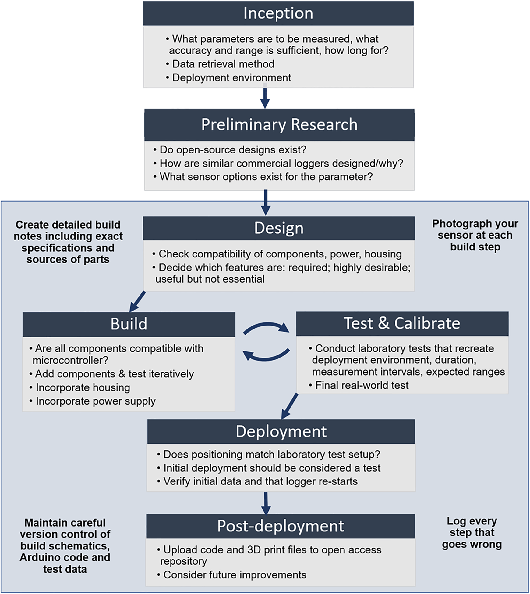
A schematic visualisation of our workflow for developing low-cost environmental monitoring devices and key considerations at each stage.
3.2 Common pitfalls
Though we outline our recommended workflow above, it is essential to bear in mind the following common pitfalls for successful deployment.
3.2.1 Testing and calibration
Unsurprisingly, testing and calibration are crucial. Our experiences show that testing must follow the deployment protocol as closely as possible. This has implications during the build and programming phases. For example, a sensor that successfully logs at 1-min intervals during lab testing offers no guarantee that switching to, say, 30-min intervals upon deployment will be faultless. Some Arduino libraries helpfully supply one line of code to set measurement intervals, but we found more substantive edits were often required when combining sensors, particularly when power-down commands are invoked. In some cases, elaborate apparatus needed to be constructed in a laboratory to mimic real-world conditions (e.g. the wind-blown sand laser-counter; Section 2.7). Calibration checks under final deployment conditions are highly recommended (Rai et al., 2017) but may be logistically problematic. Despite our geographical proximity, for example, tight regulations mean testing in the River Thames is non-trivial. On the other hand, we are fortunate that LAQN allow our Arduino sensors to be tested and calibrated at their flagship Marylebone station.
Calibration, additionally, should not be considered a one-time job. Componentry and sensor materials are subject to degradation as they age, introducing drift in reported results and potentially hampering accurate measurements (Artursson et al., 2000; Bourgeois et al., 2003). Post-processing can be implemented to correct for sensor drift through measuring standard quantities or cross-calibration against other more recently calibrated and/or accurate sensors. Moreover, cross-calibration becomes increasingly powerful as a greater density of sensors are deployed (El-Jabi and Caissie, 2019). Lastly, whilst data quality from low-cost sensors depends on careful calibration of individual sensors, the same practice applies when deploying conventional commercial instruments. Our ability to replace individual sensors in self-build designs further mitigates against sensor drift (see Section 2.5).
We recommend testing also be carried out at the component level – that is, prior to sensor assembly – as visual and electronic inspection can reveal flaws in purchased components. Wires are often mounted differently to supplied sensor schematics, for example, potentially short-circuiting the Arduino board and, at worst, posing a fire hazard. Arduino components can usually be replaced – certainly more easily than commercial loggers – but early testing saves on time, expense and frustration.
3.2.2 Time
Our experience shows clearly that every stage in a new project takes longer than pre-existing papers, instructions or even simple replication would have us believe. Repeated builds also bring an unexpected cost element. Publications showcasing the ‘build-it-yourself’ approach often present the methodology and schematics for a functioning sensor, followed by a brief reflection on accuracy and future applications (e.g. Beddows and Mallon, 2018; Khanfar et al., 2017; Metzger et al., 2018). These guides rarely comment on the time commitment, however. While this will depend on the level of technical competence and experience of the designer, the trial and error nature of designing new instruments exacerbates this issue. The water quality sensor (Section 2.4) development process illustrates this pitfall: four different models of the sensor were produced, involving numerous field and lab tests, of which two probes were successfully deployed.
There is a crucial distinction to be made between developing a new sensor and reproducing an existing design. Labour is expensive so bespoke development is a serious commitment, but reproduction vastly streamlines the time burden. A fully functioning FreeStation AWS can be constructed in 4 h, for example, but the FreeStation instructions, now online, are the result of years of testing and refining.
3.2.3 Sensor housing
Robust external housing is critical. The deployment environment will dictate the sealing effectiveness and appropriate Ingress Protection rating required for a casing, but preventing water ingress is a challenge that we underestimated repeatedly. Diagnosing the source of a leak is particularly challenging. Moreover, constructing watertight enclosures using materials in keeping with a ‘low-cost’ project adds an additional obstacle. Housing the microprocessor and associated peripherals (SD card, clock) separately from the data-collecting device may minimise leak points, even if superficially via sealing exposed components with epoxy, as implemented in our water depth logger. Liberal application of resin, silicon sealant or silicone grease is warranted, often in conjunction with cable glands or thread seal tape. Housing dimensions also need to accommodate appropriate battery options tailored to sensor power draw. Battery packs constitute up to two-thirds of the space requirements for some of our sensors, so a belated realisation that more power is necessary could necessitate a wholly new housing. We increasingly manufacture 3D-printed containers to optimise protection and streamline the design process, especially for housing smaller components. Filling gaps in commercial casings with epoxy is extraordinarily time-consuming, for example. Loose wires are a common malfunction; we advocate soldered wire connections, PCBs and the plug-and-play approach of the FreeStation to maximise durability.
Concerns around data quality have been raised regarding ad hoc housing. Terando et al. (2017), for example, identified discrepancies of up to 3°C when testing build-it-yourself Stevenson screens. Whilst this highlights a potential pitfall in the use of low-cost sensors, commercial data loggers also report substantial variance (e.g. Whittier et al., 2020). Indeed, the need for rigorous sensor-specific calibration follows best practice in environmental monitoring and is not a hurdle unique to build-it-yourself sensors. Furthermore, the capacity to deploy a higher number of sensors for equivalent financial outlay brings significant benefits through detailed cross-calibration (El-Jabi and Caissie, 2019). At the same time, there is clearly scope to promote reproduction rather than reinvention. The open-source approach of Arduino and Internet-of-Things technology could, in fact, lead to greater methodological consistency where, for example, a 3D-printer design for a Stevenson shield is shared widely amongst the research community.
3.2.4 Power
We have grappled at length with ensuring adequate power supply and maximising longevity. Think carefully about minimum measurement intervals, which will be guided by research objectives. Will a 30-min or 60-min wake-up interval provide appropriate data? What is the minimum period a sensor needs for readings to stabilise? We now have a standard core design for ultra-low-power sleeping loggers and increasingly incorporate solar-powered, rechargeable lithium ion batteries. Shaded deployment sites along riverbanks and obtaining adequate exposure in built-up areas have proved difficult. Integrating components that draw 3.3 V and 5 V is another complication, particularly when considering digital communication lines may run different voltages from sensor power voltages. Conversely, testing showed a 3.3 V Arduino Nano could drive the 5 V stepper motor on the sediment trap, which aided compatibility. There have also been notable developments around power saving in recent years across the Arduino community, involving new hardware and scripts (Beddows and Mallon, 2018; Rocket Scream, 2020). Lastly, removing obsolete LEDs from the Arduino and connected shields using a hot soldering iron or carefully slicing tracks to superfluous components with a sharp blade can reduce power draw substantially.
3.2.5 Sensor and library compatibility
Progressing from a complete assemblage of sensors, board and wires to an operating, reliable instrument is easily underestimated. One of the biggest hurdles we repeatedly encounter is a lack of compatibility between sensors and Arduino libraries when designing multiprobes. Each additional component introduces a non-linear degree of added complexity, with conflicting libraries a common occurrence. For our aquatic multiprobe, individual sensors were accurately calibrated but daily means did differ when integrated into a single instrument. We attributed these issues to electrical interference, which requires targeted compensation (Siragusa and Galton, 2000) and significantly longer build and testing times. Similarly, whilst most PM sensors use laser scattering, internal differences between manufacturers produce unique biases. These are rarely clear in supplied documentation.
3.2.6 Deployment considerations
We also emphasise that deployment protocol is a non-trivial aspect that is rarely afforded due consideration. After the more arduous task of designing, building and calibrating low-cost environmental loggers, deployment seems the simple and exciting job. This is a particular issue when sensors are handed from makers – who may know the particularities of the logger and sensor setup – to fieldworkers. Without adequate consideration of the deployment criteria of specific sensors (e.g. under what conditions does the sensor accurately measure? What periodic maintenance is required? Where specifically should the sensor be mounted?) results may pay a disservice to the effort expended in design and development. This reinforces the need to share understanding of the sensors, loggers and fieldwork conditions between makers/electronic engineers and fieldworkers. General good-practice guidance for attaining accurate measurements of the particular environmental parameter should also be adhered to.
IV Attribution and intellectual properties
The open-source revolution greatly enables customisation, enhancement and collaborative efforts within technological development through making software and hardware designs accessible and implementable. Those of us in the academic sphere, however, necessarily require attribution to ensure we as researchers are recognised for our contribution to encourage the conceptual and theoretical development of research whilst ensuring this development can still be logically tracked. Though a number of OSH journals have recently been released – for example, Sensors (launched 2001), HardwareX (launched 2017), Journal of Open Hardware (launched 2017) – journals focused on the more traditional scientific disciplines remain the preferred publishing destination for many users of build-it-yourself hardware. The majority of scientific journals in geographical and environmental fields however are clearly not geared towards technological design or hardware; thus, while instructions or design descriptions are generally included in methodological sections of journal articles, alternative methods may be required for storing computer-aided design (CAD) files, board designs, source codes, and build or calibration instructions.
We would encourage academic authors to host build instructions and materials on widely used public-facing open-source sites wherever possible. Helpfully, a range of suitable online repositories now exist, the most common being Github (a more software-focused online repository), PublicLab (focused on technologies or methodologies of measuring environmental quality parameters), Thingiverse (hosting CAD files) and the Open Hardware Repository (focused on electronics hardware). Many of these repositories embrace aspects of open or ‘remix culture’ through enabling original source material to be ‘forked’ or ‘remixed’ – when original source material is built upon independently by developers. These improvements can then be ‘pushed’ (merged) to improve the original code. Github in particular has become ubiquitous for the sharing of source codes and designs, possessing 50 million users and over 100 million repositories (Github, 2020).
The above repositories enable collaborative efforts through the very principals of transparency, encouragement of modification, and promotion of community contribution. Here, a conflict arises between the ability to modify designs, around which the aforementioned repositories exist, and the reproducibility (and necessarily explicit version control) expected of the scientific field. Helpfully, digital object identifiers (DOIs) provide a mechanism for both recognition of sources and direction to specific versions of digital material. A DOI is a unique alphanumeric string assigned by the International DOI Foundation and associated registration agencies (e.g. Crossref – the DOI registrar used by the majority of academic publishers). Persistence is a key tenet of DOIs (International DOI Foundation, 2015), meaning very little, if any, modification is permitted to material assigned a DOI. This makes DOIs more optimal for scientific citation than adopting the web addresses of earlier repositories. Common archives that are explicitly geared towards DOI creation are the Open Science Framework, Zenodo and Figshare. We particularly promote Zenodo, which has integration with Github to allow archiving of specific versions of Github repositories, thus benefitting from the vast user-base and exposure that Github offers. Note additionally, however, that many research councils (UK and abroad) now require that funded project data are uploaded to their data repositories, which can often be assigned a DOI.
Some awareness of licences should be considered essential in sensor development. The open hardware and software community have grown to embrace this aspect, but navigating the options can be puzzling. It is important developers understand that just because codes and/or designs are available online, this does not make them free to use. From a hardware perspective, Arduino has adopted the Creative Commons Attribution-ShareAlike (CC BY-SA), in brief meaning anyone can recreate the hardware, though Arduino need to be credited and derivative hardware designs must be made available under the same licence. From a software perspective, use of the standard Arduino IDE and Arduino libraries is covered by the GNU Lesser General Public License (LGPL), meaning firmware designed with non-modified versions of these does not require sharing if the firmware is not designed to relink to newer versions of either Arduino core or libraries. Modification of the Arduino IDE is required to be shared under the General Public License of the IDE, whilst modification of the Arduino environment (i.e. the initial firmware uploaded to the microcontroller) or Arduino libraries is required to be shared under the LGPL. It is important to note that third-party libraries or environments will likely have separate licensing agreements that must be individually consulted. Similarly, licensing rules differ for commercial applications. Where no specification of a licence is given, licensed usage should not be assumed.
Choosing a licence under which to release your own codes and schematics is also a complex topic, requiring consideration of what exactly is being licensed (software, hardware and/or schematics), permissions for future use of your work (e.g. non-commercial applications only), whether attribution is required, and protection of your future rights, in addition to abiding by the original licensing rules of any material that you incorporate into your designs. Hundreds of licences now exist, and the nuances of these licences clearly exceed the scope of this paper. We, however, recommend three particularly useful resources: Software Licenses in Plain English (tldrlegal.com), choosealicense.com and The Legal Side of Open Source (opensource.guide/legal).
V Summary
In this paper we have showcased the ability of low-cost sensors to transform environmental monitoring of aquatic, terrestrial and atmospheric systems around the world. By providing full design schematics, code and guidance on purchasing the components on our Github repository (https://github.com/KCLGeography/environmental-monitoring), we intend this paper to act as a catalyst for geographers and environmental scientists to embed low-cost, build-it-yourself sensors into their research programmes. Deriving insight from six case studies, including the global FreeStation hydrometeorological network (www.freestation.org), we have demonstrated the potential for low-cost sensors powered by Arduino across a wide range of disciplines including atmospheric science, ecology, geomorphology and hydrology. By drawing on 6 years’ experience, we have also highlighted potential pitfalls in design and construction, recommendations for best practice have been proposed, and a workflow for developing new sensors and overcoming technical challenges has been presented. In this paper, we have also evaluated the performance of our Arduino sensors and found strong performance in each case, reporting mean bias errors below 20%. This confirms that electronic sensors designed and constructed for a fraction of the conventional commercial cost can deliver research-grade data, particularly where greater granularity is required. Data quality depends on careful calibration that must be carried out on a sensor-specific basis; this equally follows best practice when using conventional commercial instrumentation. Given global funding pressures in science, low-cost sensor networks have the potential to deliver important benefits through improved representation of spatial and temporal variability as well as customisability – that is, the opportunity to develop sensors tailored to a particular research need or physical setting. Our experience has demonstrated that the Arduino and Internet-of-Things technology and supporting communities are sufficiently developed to allow geographers and environmental scientists with no background in electronics and limited coding experience to build new sensors. The potential for sensor development is essentially limited only by imagination, as examples of open-source Geiger counters and Arduino-based CubeSat satellites demonstrate (Geeroms et al., 2015; SeedStudio, 2011). Our workflow, schematics, code and tools for web integration (e.g. FreeStation) presented in this paper establish a framework for enhancing environmental monitoring and management from the local to global scales.
Footnotes
Acknowledgements
We thank the two anonymous reviewers for their careful, comprehensive and constructive reviews, which have allowed us to greatly improve the paper. We are grateful to a number of funders. Numerous KCL Geography and London School of Economics Department of Geography and Environment undergraduate and postgraduate students have supported, inspired and made vital contributions to our low-cost sensor development. For this paper we thank, in particular, Alex Blair, Nicole Cowell, Abbey Wong and Harriet Wilson.
Thanks to Dr Massimo Lupascu and Hasan Akhtar (National University of Singapore) for their assistance with deploying and maintaining the water table depth probes.
Author contributions
Daniel Schillereff and Kristofer Chan contributed equally to leading the writing of this paper.
Declaration of conflicting interests
The author(s) declared no potential conflicts of interest with respect to the research, authorship, and/or publication of this article.
Funding
The author(s) disclosed receipt of the following financial support for the research, authorship, and/or publication of this article: the Natural Environmental Research Council and the Arts & Humanities Research Council (grant number NE/R017999/1), the Economic and Social Research Council (grant number ES/R002126/1), the King’s College London (KCL) Undergraduate Research Fellow programme, the KCL Faculty of Social Science and Public Policy for a Research Grant, a KCL Education Grant, and a KCL Widening Participation Grant, and the London School of Economics for a Learning Technology and Innovation Ignite! grant and a Pro-Director for Education Vision Fund grant, AmbioTEK Community Interest Company (![]() ), and the Nature Insurance value: Assessment and Demonstration (NAIAD) project of the European Commission's H2020 programme (grant agreement: 730497).
), and the Nature Insurance value: Assessment and Demonstration (NAIAD) project of the European Commission's H2020 programme (grant agreement: 730497).