
Abstract
Supraglacial lakes (SGLs) are now known to be widespread in Antarctica, where they represent an important component of ice sheet mass balance. This paper reviews how recent progress in satellite remote sensing has substantially advanced our understanding of SGLs in Antarctica, including their characteristics, geographic distribution and impacts on ice sheet dynamics. Important advances include: (a) the capability to resolve lakes at sub-metre resolution at weekly timescales; (b) the measurement of lake depth and volume changes at seasonal timescales, including sporadic observations of lake drainage events and (c) the integration of multiple optical satellite datasets to obtain continent-wide observations of lake distributions. Despite recent progress, however, there remain important gaps in our understanding, most notably: (a) the relationship between seasonal variability in SGL development and near-surface climate; (b) the prevalence and impact of SGL drainage events on both grounded and floating ice and (c) the sensitivity of individual ice shelves to lake-induced hydrofracture. Given that surface melting and SGL development is predicted to play an increasingly important role in the surface mass balance of Antarctica, bridging these gaps will help constrain predictions of future rapid ice loss from Antarctica.
I Introduction
Supraglacial lakes (SGLs) form when meltwater accumulates in topographic depressions on top of glaciers, ice sheets and ice shelves, primarily during the ablation season (Echelmeyer et al., 1991). They are an important component of ice sheet hydrology because they can influence ice sheet dynamics in one of three ways (Bell et al., 2018; Das et al., 2008). Firstly, their albedo-lowering effect can intensify surface melt and induce a warming effect on the adjacent ice column (Lüthje et al., 2006; Tedesco et al., 2012; Hubbard et al., 2016). Secondly, their rapid drainage via hydrofracturing can deliver meltwater pulses to the ice sheet bed. It is well-known that SGL drainage causes transient accelerations in grounded ice velocity on the Greenland Ice Sheet (Bartholomew et al., 2010; Das et al., 2008; Schoof, 2010; Tedesco et al., 2013; Zwally et al., 2002), and recent work has shown similar effects on the Antarctic Peninsula (Tuckett et al., 2019). Thirdly, SGLs may be an important precursor for ice shelf collapse (Banwell et al., 2013; Glasser and Scambos, 2008; Scambos et al., 2003). On the Antarctic Peninsula, for example, the filling and drainage of SGLs induces ice shelf flexure and triggers widespread fracturing and disintegration (Banwell et al., 2013, 2014, 2019; van den Broeke, 2005; Glasser and Scambos, 2008; Rott et al., 1996; Scambos et al., 2009). Ice shelf disintegration plays a major role in ice sheet dynamics because the resulting loss in buttressing accelerates inland ice flow, increasing the ice discharge (Fürst et al., 2016; Glasser et al., 2011; Scambos et al., 2004).
Despite an abundance of SGL research focusing on the Greenland Ice Sheet (GrIS) (Chu, 2014), much less is known about the role of SGLs in Antarctica. However, advances in satellite remote sensing capabilities since the 1970s have revealed that SGLs are present not only on Antarctic Peninsula ice shelves (Banwell et al., 2014; Hubbard et al., 2016; Luckman et al., 2014; Scambos et al., 2000, 2003, 2009), but are also far more widespread than previously thought around the margins of Antarctica, including the periphery of the East Antarctic Ice Sheet (EAIS) (Figure 1) (Kingslake et al., 2017; Langley et al., 2016; Lenaerts et al., 2017; Moussavi et al., 2020; Stokes et al., 2019).
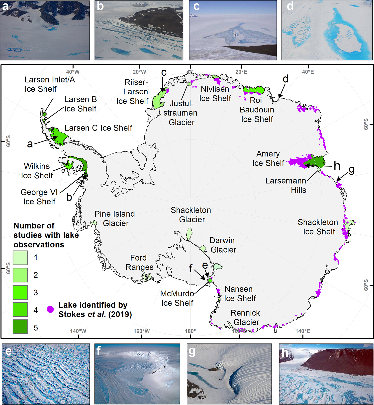
Locations around Antarctica where supraglacial lakes have been observed, together with examples: (a) Larsen C Ice Shelf, (b) George VI Ice Shelf, (c) Riiser-Larsen Ice Shelf, (d) Langhovde Glacier, (e) Ross Archipelago, (f) McMurdo Ice Shelf, (g) Sørsdal Glacier, (h) Mawson Glacier. Green shaded regions in the central map represent the number of published studies reporting supraglacial lakes in that location. Note that the number of studies reporting lakes in a given location does necessarily correspond to the number of lakes forming, or how long lakes have been present in this location. Lakes mapped in January 2017 in a recent East Antarctic assessment by Stokes et al. (2019) are shown in purple. Images reproduced from: Martin Truffer, University of Alaska Fairbanks (a), Frithjof C. Küpper, University of Aberdeen (b), Matti Leppäranta, University of Helsinki (c), Takehiro Fukuda, Hokkaido University (d), NASA Operation IceBridge (e), Chris Larsen, NASA Operation IceBridge (f), Sarah Thompson University of Tasmania (g), and Richard Stanaway, Australian National University (h).
We review how satellite remote sensing developments have transformed our understanding of the distribution and characteristics of SGLs in Antarctica, including their potential impact on ice sheet mass balance. Following a brief overview of SGL formation in Section II, Section III highlights how satellite remote sensing has advanced our understanding of Antarctic SGLs, specifically the progress in detecting and quantifying SGL distributions, volumes and their evolution through the melt season. Section IV provides an Antarctic-wide synthesis of SGL characteristics and their potential impact on ice dynamics. In Section V we identify some important gaps in understanding and suggest possible directions for future research.
II Controls on supraglacial lake formation in Antarctica
SGLs form seasonally in Antarctica when an energy surplus at the ice surface causes ice to melt (Fitzpatrick et al., 2013; Trusel et al., 2012). The spectral albedo of liquid meltwater (∼0.4–0.6) is approximately half of snow-covered ice (Figure 2) (Box and Ski, 2007; Tedesco, 2014), which leads to a positive feedback, whereby the lower albedo of the SGLs enhances melting and can lead to further increase in lake area and depth (Banwell et al., 2015; Morriss et al., 2013; Tedesco et al., 2012). For meltwater to pond in SGLs in areas of firn cover, percolation into the near-surface firn layer must be impeded by firn over-saturation or refrozen englacial meltwater (Alley et al., 2018; Harper et al., 2012; Hubbard et al., 2016; Lenaerts et al., 2017; Reynolds and Smith, 1981).
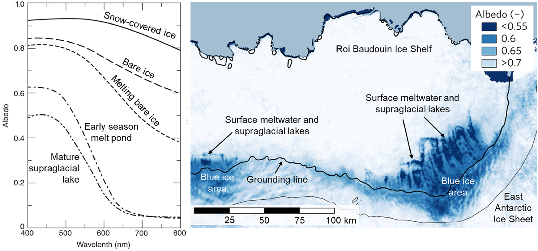
(a) Spectral albedos for a sequence of snow-covered ice to mature supraglacial lake through a melt season. Modified from Tedesco (2014). (b) Summer albedo derived from MODIS imagery on the Roi Baudouin Ice Shelf. Grounding line is represented as the thick black line. Modified from Lenaerts et al. (2017). For interpretation of the references to colours in this figure legend, refer to the online version of this article.
The location of surface depressions on the ice sheet is an important influence on where SGLs form (Echelmeyer et al., 1991). On grounded ice, topographic undulations in subglacial bedrock are translated into ice surface depressions, which lakes tend to re-occupy in the same location annually (Echelmeyer et al., 1991; Ignéczi et al., 2016, 2018; Langley et al., 2016). On slower-moving ice that is grounded, SGLs often grow larger and deeper than those on floating ice further downstream (Banwell et al., 2014; MacDonald et al., 2018; Sergienko, 2013). This is because lakes tend to re-occupy surface depressions for longer, allowing them to expand and deepen by lake bottom ablation, and are often fed by surface channels that increase lake catchment areas (Das et al., 2008; Leeson et al., 2012; Tedesco et al., 2012). The surface of slower-moving, thicker ice also supports larger, smoother undulations compared to thinner, faster-flowing ice (Gudmundsson, 2003) and is less likely to be subject to crevassing. In contrast, lakes on floating ice form in surface depressions that migrate with ice flow (MacDonald et al., 2018). These surface depressions are produced in response to spatial and seasonal variations in ice flow, ice thickness and ice flexure (Banwell et al., 2019). Surface depressions are also controlled by the location of basal channels that are incised by sub-surface melting (Dow et al., 2018) and basal crevasses (McGrath et al., 2012) because thinner ice in these regions that has reached hydrostatic equilibrium will sit lower in the water. Surface depressions can also be associated with flow stripes, shear-margins and suture zones (Banwell et al., 2014; Bell et al., 2017; Ely et al., 2017; Glasser and Gudmundsson, 2012; Luckman et al., 2014; Reynolds and Smith, 1981). Reduced firn air content and ice surface topography are therefore first-order controls on SGL locations.
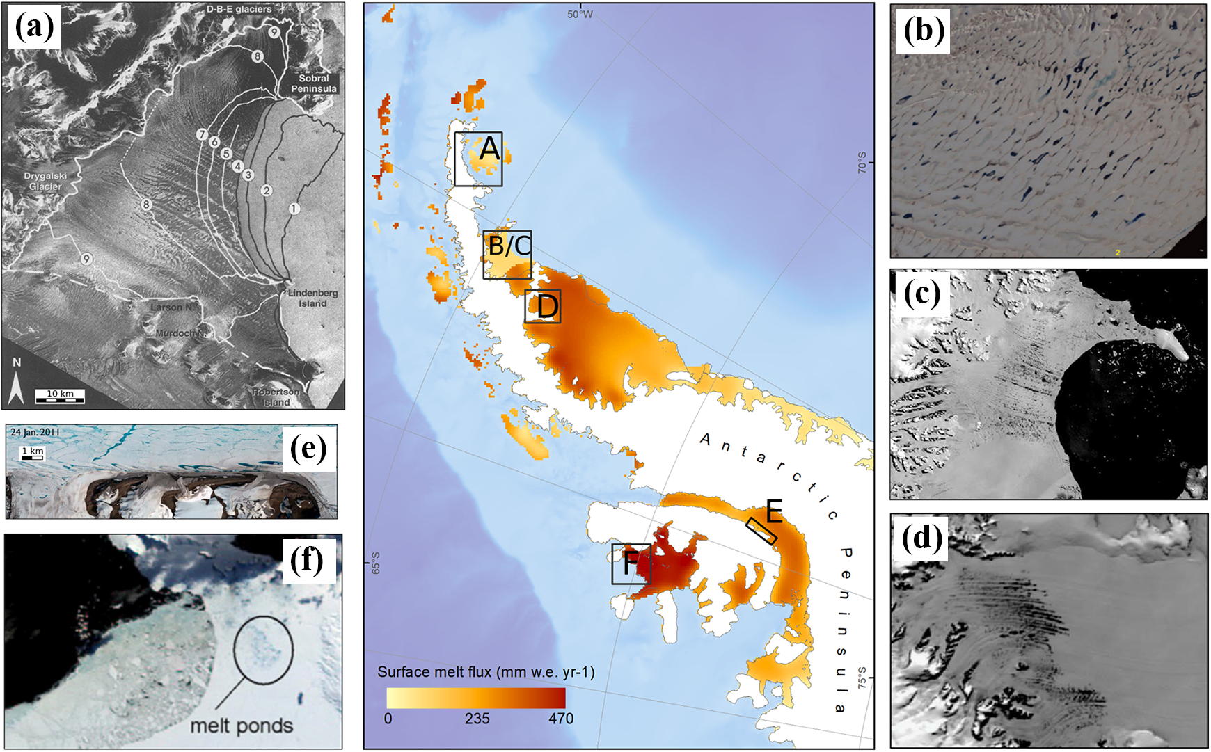
In Antarctica, it has been noted that glaciological and climatic conditions around ice shelf grounding lines (i.e. where the ice begins to float) are conducive to SGL formation (Kingslake et al., 2017; Lenaerts et al., 2017; Stokes et al., 2019). The majority of SGLs form on ice shelves close to and just downstream of the grounding line because the lower elevations and large decrease in ice surface slope are conducive to meltwater ponding (Stokes et al., 2019). SGL distributions across Antarctica have been shown to reflect the complex interplay between local and regional wind patterns, ice surface topography and albedo (Kingslake et al., 2017; Lenaerts et al., 2017; Stokes et al., 2019). Figure 3 plots SGL locations and surface melt flux together with blue ice areas, rock outcrops, wind scour zones and near-surface wind speeds, which shows that the highest densities of SGLs do not necessarily coincide with regions of highest surface melt (Datta et al., 2019; Kingslake et al., 2017; Lenaerts et al., 2017; Trusel et al., 2013). On the Antarctic Peninsula, for example, the strength and frequency of westerly föhn winds dictate SGL distribution, resulting in intense melting (>400 mm w.e. yr –1) and localised ponding on ice shelves, even in Antarctic winter (Figure 3a) (Datta et al., 2019; Lenaerts et al., 2017; Luckman et al., 2014; Kuipers Munneke et al., 2018; Trusel et al., 2013; Wiesenekker et al., 2018). Likewise, in coastal East Antarctica, SGLs are often clustered near ice shelf grounding zones, whereas they are often absent further downstream despite higher surface melt fluxes (Figure 3b, 3c, 3d). Higher accumulation and firn air content in near coastal regions likely explain this absence, because surface meltwater can percolate into the firn before it can pond on the surface (Lenaerts et al., 2017). Warm air delivery to grounding zones from persistent katabatic winds exposes lower-albedo blue ice through wind scouring, which intensifies melting and ponding (Lenaerts et al., 2017)
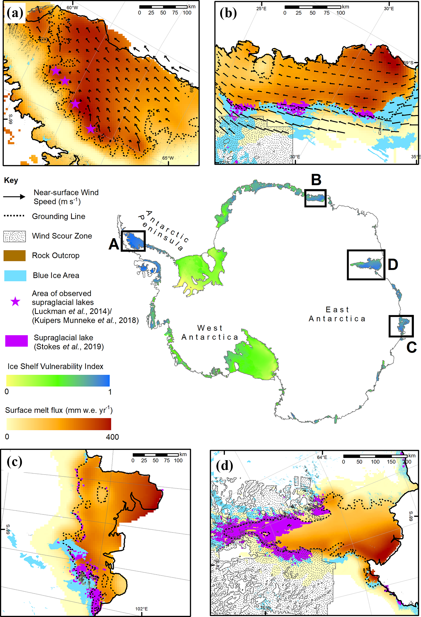
Distribution of near-surface wind speed, wind scour zones, exposed rock, blue ice, surface melt flux, ice shelf vulnerability to surface-melt-induced collapse, and supraglacial lakes (from January 2017). Surface melt fluxes are derived from QuickScat scatterometer (2000–2009 average, Trusel et al., 2013) and include meltwater that could refreeze in the snow/firn. Ice shelf vulnerability is derived from QuikSCAT data and represents the relative concentration of refrozen meltwater in the firn (Alley et al., 2018). The grounding line and coastline are represented by dotted and solid black lines respectively. Arrows represent near-surface wind speed vectors (Lenaerts et al., 2017; Luckman et al., 2014). Supraglacial lake datasets are reproduced from Stokes et al. (2019). On Larsen C Ice shelf (A), supraglacial lake formation is restricted to inlets (blue stars), driven by föhn-enhanced melting. On Roi Baudouin Ice Shelf (B), lakes clustered at the grounding zone are associated with katabatic wind-enhanced melting. The co-occurrence of lakes with rock outcrops and wind-scoured blue ice is prominent on other East Antarctic ice shelves, such as Shackleton (C) and Amery (D).
In summary, SGLs are widespread around the periphery of Antarctica and form predominantly on floating ice shelves, clustered a few kilometres down-ice from the grounding line. The occurrence of SGLs is controlled by firn air content, as well as by short-lived föhn wind events or persistent katabatic winds that intensify surface melting.
III Satellite remote sensing of supraglacial lakes
The revolution in satellite remote sensing capabilities since the 1970s has significantly improved our overall understanding of SGLs in Antarctica. This is reflected in the growing number of SGL studies in the last decade (Figure 4; Table 1), with the vast majority taking advantage of increasingly plentiful, openly available optical satellite imagery (Figure 5). Table 1 highlights the progression in remote sensing-based assessments of SGLs in Antarctica, from the visual identification of lakes in earlier coarser optical and radar satellite imagery, to manual delineation of lake extents from medium resolution imagery, to semi-automated classification of lakes and extraction of lake characteristics such as areas, depths and volumes from high-resolution optical imagery. A trade-off exists between resolution, return period and swath width when selecting satellite imagery for investigating SGLs (Table 2) (Leeson et al., 2013). The integration of imagery from multiple sensors can, therefore, exploit their respective benefits for assessments of SGL evolution during and between melt seasons.
Published remote sensing-based assessments of supraglacial lakes and other supraglacial features on Antarctica (in chronological order of publication date).
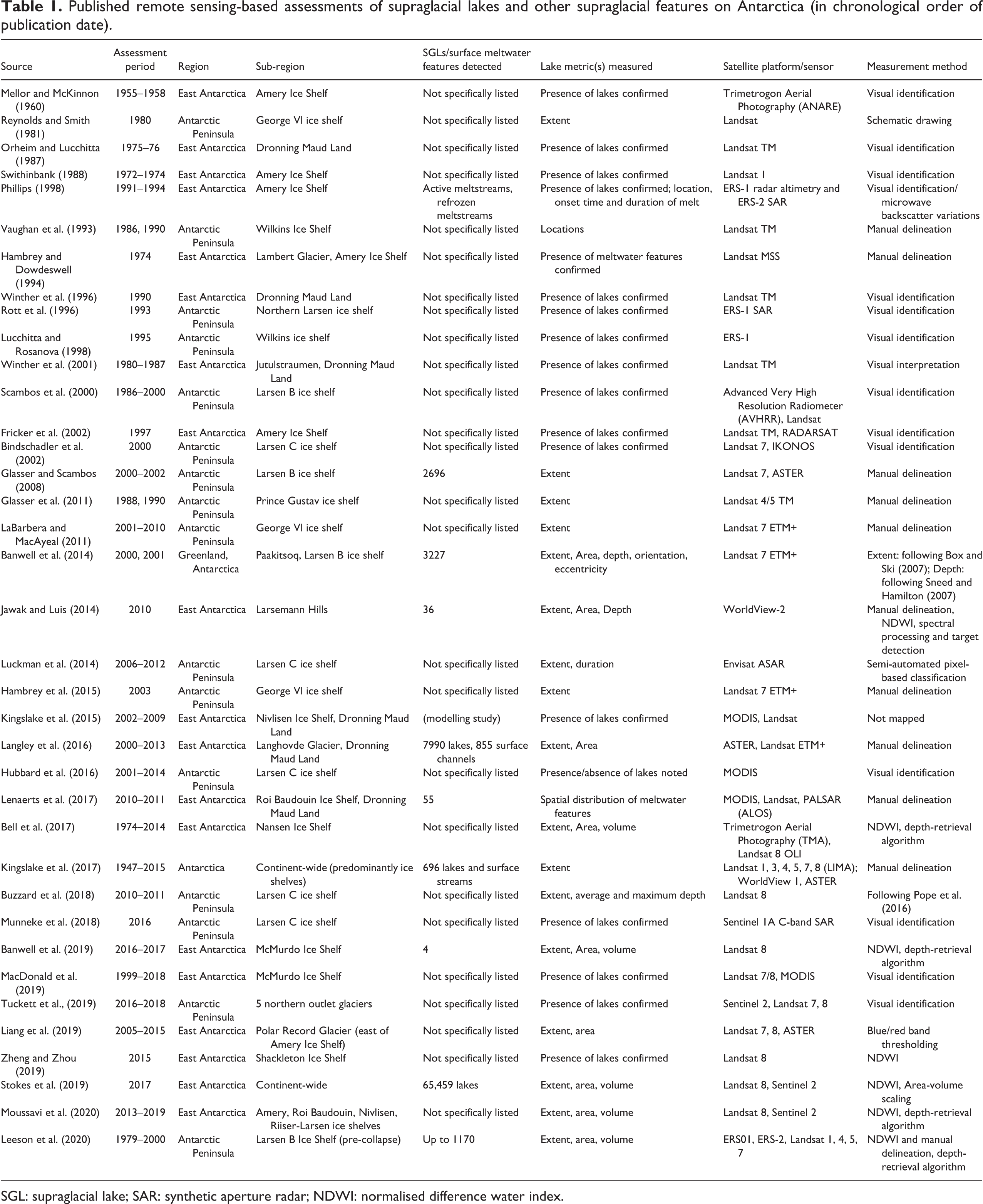
SGL: supraglacial lake; SAR: synthetic aperture radar; NDWI: normalised difference water index.
A comparison of different optical and radar satellite remote sensing approaches for detecting, measuring and monitoring supraglacial lakes in Antarctica.
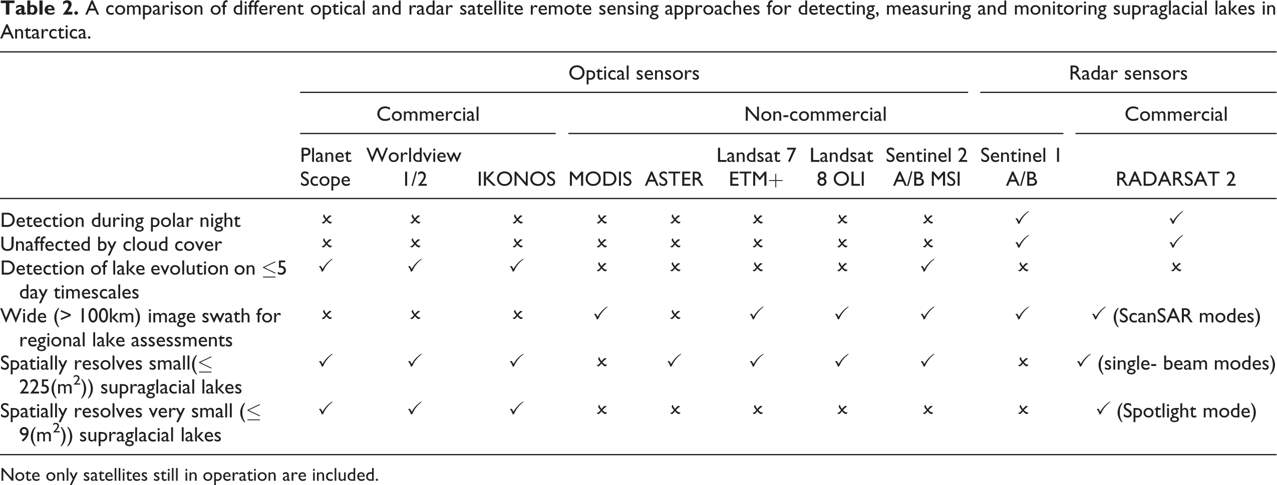
Note only satellites still in operation are included.
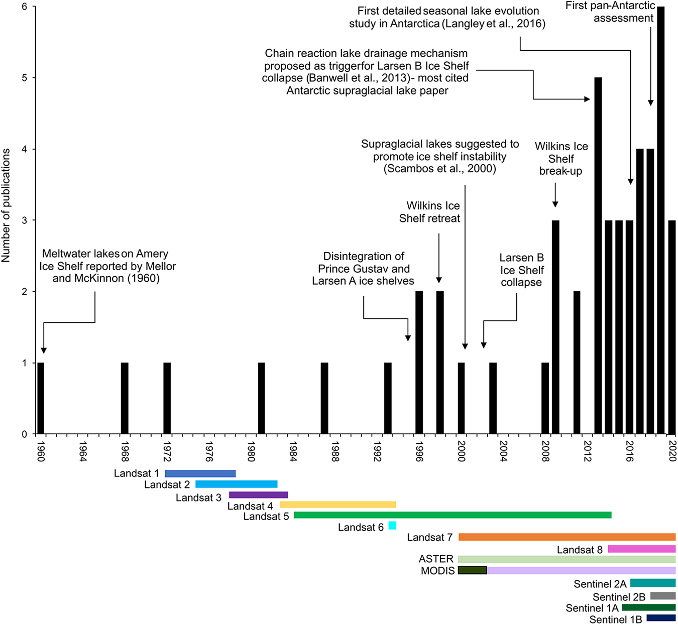
The number of Antarctic-focused published studies containing the keywords ‘Antarctic’ and ‘supraglacial lake’ or ‘melt pond’ or ‘melt lake’ from a combined search of the ISI Web of Science catalogue (n = 49, search date: 15th January 2020, glaciological studies only). Coloured bars represent operational periods of common multispectral and radar satellites that have been employed in SGL studies. Earlier studies reported field and remote sensing observations of supraglacial lakes on several Antarctic ice shelves (Amery, George VI, Justulstraumen/Fimbul) and, more recently, were motivated by the rapid disintegration of Antarctic Peninsula ice shelves. The first notable peak in 2009 coincides with the disintegration of the Wilkins Ice Shelf. The second most productive year in 2013 coincides with the first study to propose an explanatory mechanism for the synchronicity of lake drainages on Larsen B Ice Shelf prior to its collapse. The increase in publications since this date also coincides with the launch of higher resolution multispectral and radar satellites, notably Landsat 8 and the Sentinel constellations (see Figure 5).
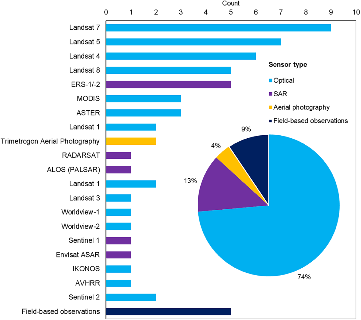
Most commonly applied remote sensing imagery sources for measuring and monitoring supraglacial lakes in Antarctica, along with field-based studies. SAR: synthetic aperture radar
3.1 Coarse (>250 m) spatial resolution sensors
The comparatively coarse spatial resolution (0.25–1.09km) and wide swath (2330–2990km) MODerate-resolution Imaging Spectroradiometer (MODIS) and Advanced Very High Resolution Radiometer (AVHRR) sensors have been used to map SGL distributions at the regional scale, e.g. including large ice shelves (Hubbard et al., 2016; Lenaerts et al., 2017; MacDonald et al., 2019). For example, on the Antarctic Peninsula, MODIS has been used to highlight the presence of ice dolines (drained lake basins) on Larsen B Ice Shelf before its collapse (Bindschadler et al., 2002), and to show that SGLs persist over decadal timescales on parts of Larsen C Ice Shelf (Hubbard et al., 2016). In East Antarctica, MODIS has also been used to confirm the presence of SGLs during summer in the grounding zone of the Roi Baudouin Ice Shelf (Lenaerts et al., 2016). The sub-daily repeat coverage of AVHRR has lent itself to documenting the presence of SGLs on Antarctic ice shelves before their break-up, including Wilkins and George VI ice shelves (Scambos et al., 2000). That said, frequent cloud coverage was found to reduce its temporal coverage to twice a month, preventing detailed analysis of lake extents or drainage (Scambos et al., 2000). The wide swath coverage of these two sensors comes at the expense of a coarser spatial resolution, resulting in the inability to accurately resolve SGLs below the pixel resolution (<0.0625km2 for MODIS, <1.18km2 for AVHRR). Given the tendency of Antarctic SGLs to be shallower and narrower than those on the GrIS (Banwell et al., 2014), this lower spatial resolution may bias the detection of rapid drainage events by missing smaller or rapidly draining lakes (Cooley and Christoffersen, 2017). In summary, the wide swath and rapid revisit period of coarse resolution sensors make them well-suited to continent- or region-wide studies, as well as those requiring high temporal frequency.
3.2 Medium (15–250m) spatial resolution sensors
Over 20 Antarctic SGL studies have exploited the Landsat suite of satellites (Figure 5; Table 2). In early studies, lakes were identified in Multispectral Scanner (MSS) imagery (60m resolution) on Justulstraumen (upstream of Fimbul Ice Shelf; Figure 1), but their area could not be accurately resolved (Orheim and Lucchitta, 1987; Winther et al., 1996). The improved 30m spatial resolution and two additional infrared bands of Thematic Mapper (TM) enabled subsequent studies to better resolve individual lakes, but features such as thin lake ice coverings were still unresolvable (Orheim and Lucchitta, 1987).
More recently, studies have exploited the 15m resolution panchromatic band of Landsat-7 Enhanced Thematic Mapper Plus (ETM+) to pinpoint the timing of SGL overflow and/or refreezing (Kingslake et al., 2015) and to extract lake characteristics such as extents, areas and volumes (Banwell et al., 2014). Landsat-7 ETM+ has also been used to produce time-series of lake frequencies, areas and volumes over 13 austral summers, with a maximum temporal resolution of 13 days (Langley et al., 2016). The Landsat-7 ETM+ record has also been utilised to map SGL distributions at a continental scale (Kingslake et al., 2017: Section 4.3).
The Advanced Spaceborne Thermal Emission and Reflection Radiometer (ASTER) provides a more favourable revisit period (1–2 days) than Landsat 7 and was employed to conduct detailed mapping of filled and drained lakes on Larsen B Ice Shelf pre-, during and post-collapse (Glasser and Scambos, 2008). This rapid revisit period has also enabled individual lake disappearances and drainage mechanisms to be distinguished for the first time in East Antarctica (Langley et al., 2016).
Most recently, the Landsat-8 Operational Land Imager (OLI) has offered improved precision for mapping SGLs and extracting their characteristics, owing to its enhanced spatial (15m) and radiometric resolution (12-bit, meaning greater dynamic range), high signal-to-noise ratio and high temporal resolution (∼725 scenes per day, compared to ∼475 scenes per day from Landsat-7). This has enabled SGLs to be mapped in detail at the outlet glacier, ice shelf and pan-ice sheet scale (Bell et al., 2017; Kingslake et al., 2017; Stokes et al., 2019).
3.3 High (≤ 10m) spatial resolution sensors
High-resolution multispectral imagery provided by satellites launched within the last decade such as Sentinel-2 (10m resolution, five day revisit period), Worldview-2 (1.84m resolution, 1.1 day revisit period) and IKONOS (3.28m, three day revisit period) have enabled very small or narrow lakes to be resolved (Bell et al., 2017; Jawak and Luis, 2014; Kingslake et al., 2017; Labarbera and MacAyeal, 2011; Moussavi et al., 2020; Stokes et al., 2019). In Figure 6 we compare SGLs on a tributary glacier of Amery Ice Shelf to demonstrate the vast improvement in the ability to resolve individual SGLs. Where individual lakes were unresolvable in coarser resolution imagery (AVHRR and MODIS), the bathymetry of individual lakes and partial lake ice coverage are now detectable in more detail. High-resolution sensors also provide the capability to map narrower supraglacial channels occurring in association with SGLs, thus potentially enabling a better understanding of lake drainage mechanisms.
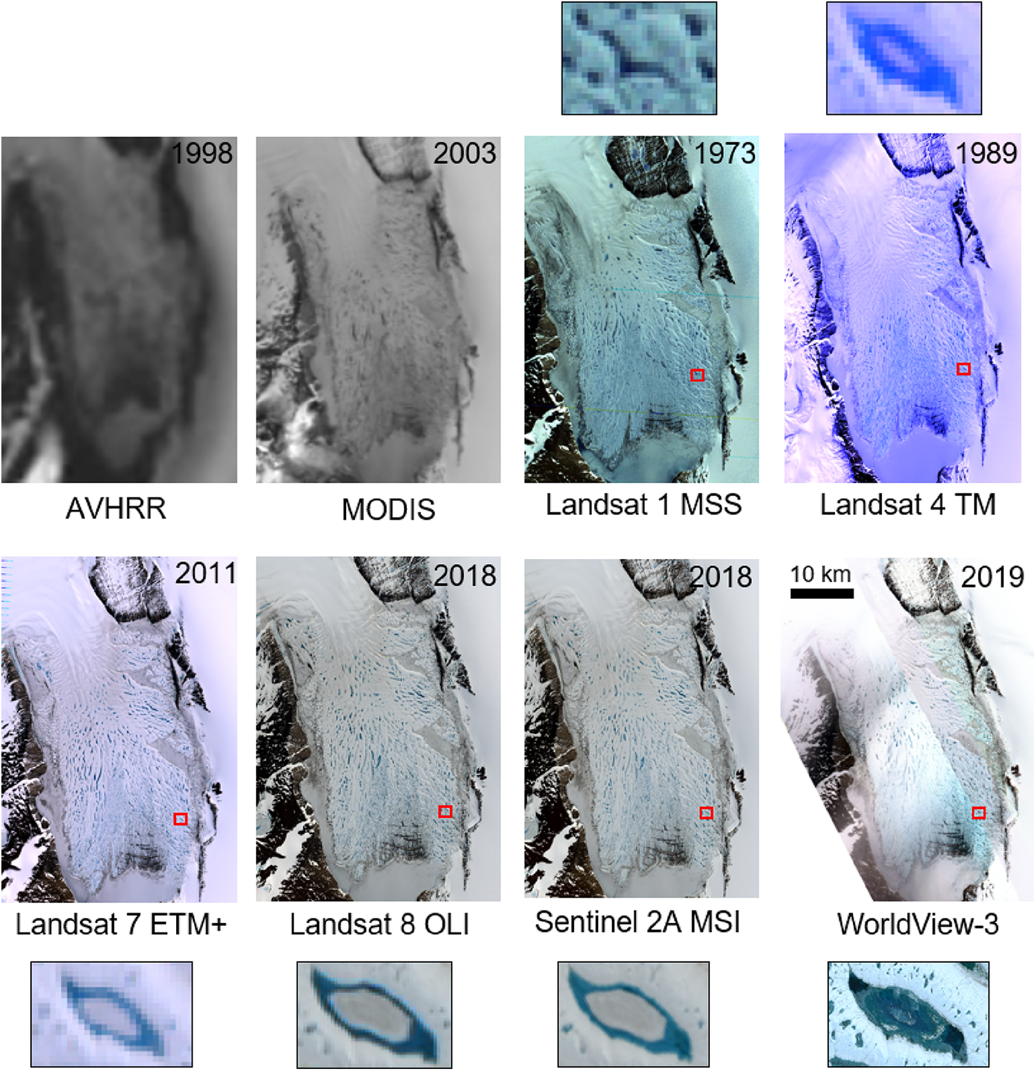
Examples of the evolution of satellite image sensor resolution and detection of supraglacial lakes on Beaver Lake, an epishelf lake adjacent to Amery Ice Shelf, East Antarctica. Panels moving from top left to bottom right represent satellite sensors in order of increasing spatial resolution. Smaller insets adjacent to six of the panels show the same supraglacial lake to demonstrate the improvement in detail. The ability to resolve supraglacial lake extent, including very small and narrow ponds, has vastly improved since coarser sensors like AVHRR and MODIS, which were unable to distinguish these features. Most recently, high (>10m) resolution sensors such as Sentinel 2 MSI and Worldview-3 can resolve lake bathymetry and surface features such as partial lake ice coverage. Imagery: Scambos et al. (1996); United States Geological Survey; Google, Maxar Technologies.
Despite the improvement in spatial resolution, the five-day revisit period under cloud-free conditions provided by the Sentinel-2A/B constellation precludes the identification of the precise onset of SGL formation and the tracking of SGL behaviour (and possible rapid drainage) on daily to sub-daily timescales (Quincey and Luckman, 2009; Stokes et al., 2019; Williamson et al., 2018). Recent pan-ice sheet assessments and studies tracking and quantifying meltwater depth and volume in individual lakes have maximised the combined potential of Landsat-8 and Sentinel-2 by increasing the number of available cloud-free scenes from which to map SGLs (Kingslake et al., 2017; Leeson et al., 2015; Miles et al., 2017; Moussavi et al., 2020; Stokes et al., 2019). Daily commercial satellite imagery provides a highly valuable addition, though its restrictive cost and limited swath width (<20km) have tended to limit its use to smaller areas. However, up to 10,000km2 imagery per month is freely available for research purposes from the recently launched PlanetScope satellite constellation (Planet Team, 2020). The substantially higher spatial (0.8–5m) resolution and daily revisit period of this imagery offers excellent potential for more accurately characterising SGL onset, growth and drainage mechanisms, although Planet imagery has yet to be used in Antarctica for this purpose.
3.4 Synthetic aperture radar (SAR) imagery
The most important limitations to optical satellite sensors, however, remain cloud cover and their inability to image during polar night (Quincey and Luckman, 2009). SAR removes the need for clear-sky imagery, daylight and the high solar zenith (Luckman et al., 2014) because it is an active sensor that transmits electromagnetic radiation, meaning data can be collected in winter (Miles et al., 2017; Kuipers Munneke et al., 2018). ERS-1-2, Radarsat and Envisat SAR imagery have successfully detected refrozen lakes and melt streams on the Amery Ice Shelf in August, and on the Wilkins and northern Larsen ice shelves in July (Fricker et al., 2002; Lucchitta and Rosanova, 1998, Phillips, 1998; Rott et al., 1996). Wintertime surface ponding was linked to föhn wind events on the Larsen C Ice Shelf using recently launched Sentinel-1A C-band SAR (Kuipers Munneke et al., 2018). Sentinel-1 provides a promising means of tracking SGL growth and drainage through melt seasons into the winter (Miles et al., 2017) and this is an important area for future SGL research in Antarctica. However, undulating topography can be problematic for SAR, because this creates radiometric distortion that fails to detect small, narrow SGLs (Johansson and Brown, 2012). Backscatter associated with high surface roughness (e.g. in areas of complex terrain with wet snow and firn) also poses difficulties for lake detection under certain polarisation (horizontal transmit and horizontal receive, HH) (Miles et al., 2017). In summary, SAR provides excellent potential in Antarctica for obtaining SGL observations in austral winter and for detecting sub-surface meltwater bodies associated with SGLs.
3.5 Supraglacial lake detection and mapping methods
Manual delineation of SGLs from satellite imagery in a Geographic Information System (GIS) offers a reliable method for identifying individual SGLs (Leeson et al., 2013) and for conducting detailed mapping of SGL networks on individual ice tongues and shelves (Glasser and Scambos, 2008; Langley et al., 2016). However, manual digitisation is less suitable for larger-scale assessments because it is time-intensive and can be subject to user bias (Jawak and Luis, 2014; Williamson et al., 2017). In contrast, semi and fully automated lake detection methods can be rapidly applied to hundreds of satellite scenes (Stokes et al., 2019).
The well-established Normalised Difference Water Index adapted for ice (NDWI ice) classifies water-covered pixels based on exceedance of an empirically selected red/blue reflectance threshold (typically >0.2–0.5) (Fitzpatrick et al., 2013) and has been successfully applied in East Antarctica to delineate SGLs (Bell et al., 2017; Jawak and Luis, 2014; Stokes et al., 2019). This is a pixel-based method because classification is based on spectral information of individual pixels. Additional thresholds have successfully been applied to distinguish between shallow water/slush and medium-deep water (0.12–0.14 and 0.14–0.25) (Bell et al., 2017). Lakes have also been detected on the GrIS using dynamic band thresholding, which classifies pixels as water if their red band reflectance is less than a selected threshold of the mean reflectance in a surrounding moving window (Everett et al., 2016; Selmes et al., 2011, 2013; Williamson et al., 2017). Misclassification of partially ice-covered lakes as bare ice can be problematic (Banwell et al., 2014; Sundal et al., 2009), but modified versions with elevated thresholds can eliminate false positives, such as slush zones with spectrally similar signatures to SGLs (Jawak and Luis, 2014; Moussavi et al., 2020; Yang and Smith, 2013). This can, however, exclude very shallow lakes (Miles et al., 2017). NDWI is, therefore, a rapid semi-automated method for retrieving pixel-based SGL extents, which can then be polygonised for analysis in a GIS, though the presence of slush can confound SGL classification. A new threshold-based lake classification method has been successfully applied to five East Antarctic ice shelves, combining the NDWI ice with the Normalised Difference Snow Index (NDSI) (Hall et al., 1995) to help isolate clouds and rocks (Moussavi et al., 2020). This new method was found to produce fewer misclassification errors and was able to detect shallow lakes missed using the NDWI ice alone (Moussavi et al., 2020).
Object-based classification is useful for exploiting SGL features distinguishable in very high-resolution optical imagery. Rather than classifying individual pixels, object-orientated classification focuses on differences between groups of pixels (or ‘objects’) with similar texture, tone, pattern or shape (Johansson and Brown, 2013). For example, spectral matching and target detection applied to WorldView-2 images extracted the boundaries of a small (36) sample of SGLs in the Larsemann Hills, Princess Elizabeth Land more accurately than with the NDWI (Jawak and Luis, 2014). Though non-pixel-based methods can better distinguish between lakes and slush, lakes that are small, shallow or elongated are at risk of being missed (Johansson and Brown, 2013).
3.6 Extracting supraglacial lake depths and volumes
Studies using coarser resolution Landsat-1-5 imagery were restricted to visual assessments of lake depth (e.g. Orheim and Lucchitta, 1987), but recent studies have exploited the enhanced spectral and spatial resolution of Landsat-7, Landsat-8 and Sentinel-2 to quantify estimates of SGL depths in Antarctica using a radiative transfer model (Banwell et al., 2014, 2019; Bell et al., 2017; Moussavi et al., 2020; Sneed and Hamilton, 2007). The model calculates lake water depth using the rate of light attenuation in water, lake-bottom albedo and optically deep water reflectance (Philpot, 1989):

where: z = lake depth; Ad = lake bed reflectance (approximated as pixel reflectance from lake edge); R∞ = reflectance of optically deep water (approximated as pixel reflectance from open ocean water); Rz = reflectance value, and g = attenuation co-efficient rate.
This radiative transfer model was used to extract lake depths prior to the collapse of the Larsen B Ice Shelf and provided estimates of the likelihood of lake drainage by hydrofracture (Banwell et al., 2014). The same method has been used to demonstrate the coevolution of lake area with depth over multiple melt seasons on Langhovde glacier in Dronning Maud Land (Langley et al., 2016). The transfer model makes several assumptions about SGLs: that they have negligible suspended or dissolved in-/organic particulate matter, that there is minimal wind-induced lake surface roughness, and that the lake-bottom albedo is homogenous (Moussavi et al., 2016; Sneed and Hamilton, 2011). While the last of these assumptions holds true for SGLs in Greenland (Sneed and Hamilton, 2011), it may be problematic in certain areas, such as on fine debris-rich ice (Banwell et al., 2019; Pope et al., 2016), and calibration with in-situ field-based measurements is much needed (Bell et al., 2018).
A fully automated method for extracting SGL volumes has been developed for the Paakitosq and Store Glacier regions of west Greenland (Williamson et al., 2017). This derived an area-to-volume scaling relationship across a much larger sample (n = 1114) than in previous empirically based area-depth scaling studies (Box and Ski, 2007; Liang et al., 2012). Williamson et al. (2018) applied the algorithm to detect rapid SGL drainage events during summer 2014, using a combined Sentinel-2 and Landsat-8 dataset. Recent efforts have begun deriving lake depth and volume time-series over some Antarctic ice shelves using a combined Sentinel-2 and Landsat-8 dataset (Moussavi et al., 2020). This has been used to detect individual lake drainages and to quantify seasonal lake volume changes over one ice shelf. Such an approach applied across Antarctica to produce a continental dataset of SGL volumes would provide valuable insight into seasonal SGL evolution, although partial lake ice coverage and a lack of cloud-free lake observations may present difficulties in detecting lake boundaries and in classifying rapid drainages. Initial work to quantify SGL dimensions across Antarctica has also suggested SGLs are smaller and shallower than those in Greenland (Moussavi et al., 2020; Stokes et al., 2019), highlighting the need for an ice-sheet-wide assessment of lake depths to quantify meltwater storage in SGLs across Antarctica and to constrain in which regions of the ice sheet hydrofracture drainage may occur.
IV Antarctic supraglacial lake distribution and impact on ice dynamics
We now synthesise published observations of SGLs in each major region of Antarctica. In Table 3 we provide a regional comparison of SGL characteristics that have been observed in Antarctica, including spatial distributions, depths, elevation, onset/freeze-up periods, association with supraglacial features (such as channels, dolines or moulins) and drainage behaviours.
A regional comparison of supraglacial lake characteristics that have been observed in Antarctica.
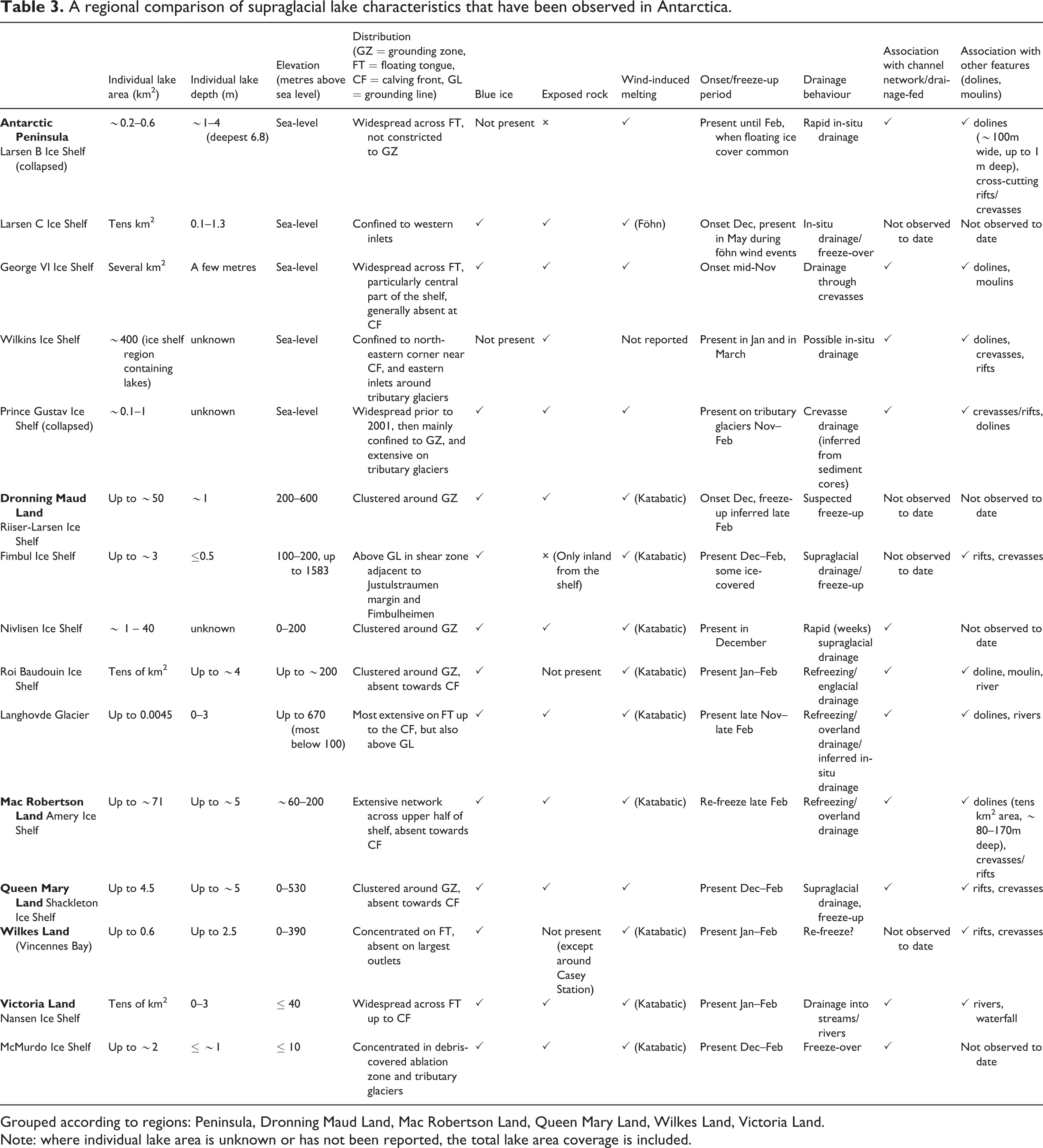
Grouped according to regions: Peninsula, Dronning Maud Land, Mac Robertson Land, Queen Mary Land, Wilkes Land, Victoria Land.
Note: where individual lake area is unknown or has not been reported, the total lake area coverage is included.
4.1 Antarctic Peninsula
Lakes have been commonly observed on most Antarctic Peninsula ice shelves, and are known to be capable of fracturing and weakening them (Figure 7) (Scambos et al., 2003; Glasser and Scambos, 2008; Glasser et al., 2011). The most notable of these events was the near-synchronous drainage of over 2750 SGLs, up to 6.8 m deep, on Larsen B Ice Shelf in the days prior to its collapse in February 2002 (Figure 8) (Banwell et al., 2014; Glasser and Scambos, 2008). Given their near-synchronous drainage in the days prior to disintegration, and their association with dolines (several hundred km2 in area and up to 19m deep) and cross-cutting rifts, these lakes are thought to have drained via hydrofracturing (Bindschadler et al., 2002; Glasser and Scambos, 2008; Scambos et al., 2000, 2003, 2009).
Examples of supraglacial lake observations on Antarctic Peninsula ice shelves prior to their disintegration or major calving. Prince Gustav Ice Shelf (A), which disintegrated in 1995; Larsen B ice Shelf (B and C), which disintegrated in 2002; Larsen C Ice Shelf (D); George VI Ice Shelf (E); and Wilkins Ice Shelf (F), which underwent major calving in 1998 and 2008. Imagery credits: (A) Rott et al. (1996), (B) Glasser and Scambos (2008), (C) National Snow and Ice Data Center, (D) Luckman et al. (2014), (E) Labarbara and MacAyeal (2011), (F) Scambos et al. (2009).
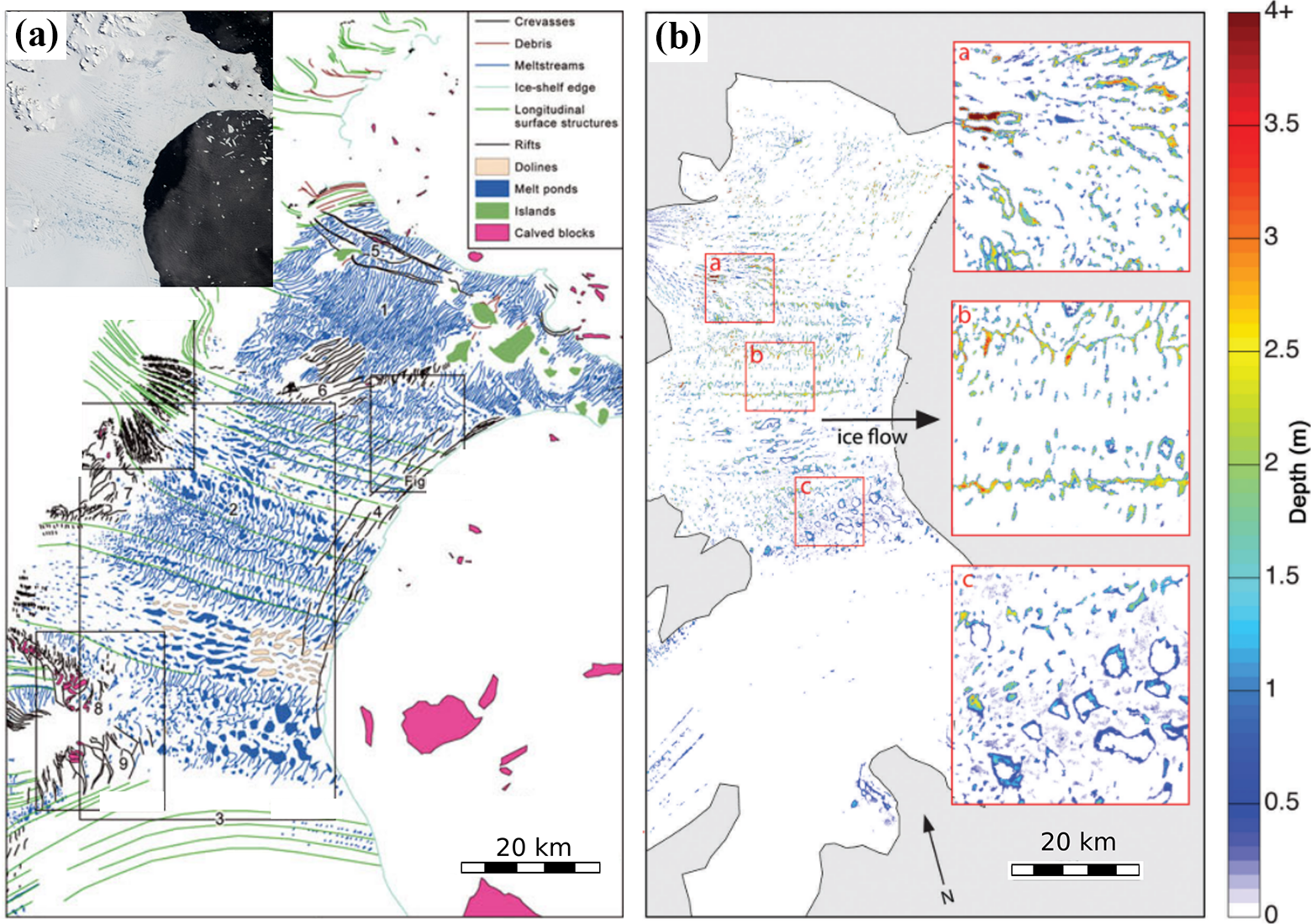
(a) Larsen B Ice Shelf surface structures in February 2002 (reproduced from Glasser and Scambos, 2008), including an extensive network of supraglacial lakes and streams that extend to the ice shelf calving front, alongside ice dolines indicating possible drained lakes. Inset shows lakes visible on the ice shelf surface from 31st January 2002. MODIS image (credit: NASA Earth Observatory). (b) Pre-collapse lake depths derived from 21st February 2000 Landsat reflectance (Reproduced from Banwell et al., 2014).
Indeed, a plausible mechanism for the fragmentation of Larsen B Ice Shelf has been modelled numerically, involving the drainage of a single ‘catalyst’ lake, which triggers a propagating fracture network able to cause progressively distal lakes to drain (Banwell et al., 2013; Robel and Banwell, 2019). This ‘chain reaction’ mechanism is based on the flexural response of ice to an applied load (i.e. meltwater in a lake) (Figure 9) (Labarbera and MacAyeal, 2011; Sergienko, 2013) and is successfully able to replicate the near-synchronous lake drainage and widespread fracture network that fragmented Larsen B Ice Shelf into unstable blocks capable of capsizing (Banwell et al., 2013). More recently, Leeson et al. (2020) showed that SGLs spread southwards on the ice shelf in the two decades preceding its collapse at a rate commensurate with meltwater saturation of its surface. However, lake deepening across the ice shelf over this period suggests this could be the result of enhanced lake bed ablation rather than the result of successive lake filling and draining (Leeson et al., 2020).
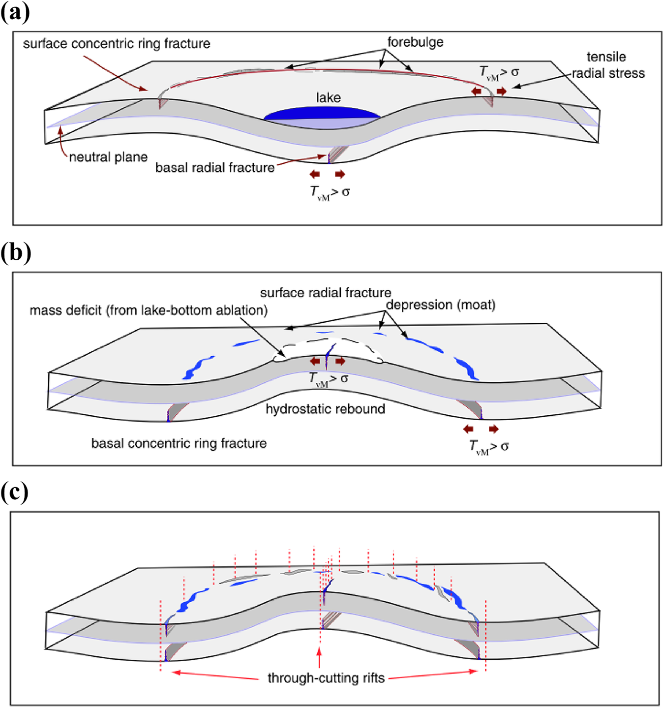
A schematic representation of the stress regime, flexural response and fracturing associated with ice shelf loading (supraglacial lake formation) and unloading (lake drainage) (reproduced from Banwell et al., 2013).
Immediately south of the former Larsen B, Larsen C Ice Shelf experiences less extensive but localised ponding, where surface melt duration has increased by up to two days per year (Bevan et al., 2018; Luckman et al., 2014). SGLs tens of metres in width and tens of kilometres in length (Luckman et al., 2014) are largely confined to western inlets fed by tributary glaciers, such as Cabinet Inlet on the Foyn Coast (Holland et al., 2011; Kuipers Munneke et al., 2018). Short-lived (<48 hr) föhn wind events (driven by episodic interaction of westerly winds with topography) intensify melt rates in these inlets and support repeated, localised ponding (Kuipers Munneke et al., 2018; Wiesenekker et al., 2018). The modelled onset of SGL growth (November) and their depths (average 1.3–1.5m) near the Larsen C grounding line correspond well with those derived from Landsat-8 imagery (Pope, 2016) when a föhn effect is added. This highlights the importance of localised climatic conditions for SGL distributions on this ice shelf (Buzzard et al., 2018b). The disappearance of hundreds of lakes in Cabinet Inlet on Larsen C over 10 days in 2003 and three weeks in 2007 is also suggestive of hydrofracture drainage (Luckman et al., 2014), as observed on Larsen B (Scambos et al., 2003, 2009). The possibility of meltwater-driven hydrofracture on Larsen C has been highlighted by 1D ice shelf model simulations of future lake distributions (Buzzard et al., 2018b). In particular, larger lakes that migrate towards the front of the Larsen C Ice Shelf under warmer atmospheric conditions may deepen sufficiently to remain unfrozen between melt seasons, thereby pre-disposing them for hydrofracture (Buzzard et al., 2018b). The depleted firn air thickness of Larsen C (0.3m in western inlets) also increases the likelihood of extensive SGL ponding and future instability, driven by sustained föhn-enhanced melting (Alley et al., 2018; Holland et al., 2011). The presence of a massive, dense ice lens in Cabinet Inlet confirms an ice-saturated firn layer conducive to SGL ponding (Hubbard et al., 2016). Thus, although not currently at imminent risk of hydrofracture-induced collapse, Larsen C may be at risk of future instability if lakes become more extensive across the ice shelf under consecutive seasons of excessive summer melting (Alley et al., 2018; Rintoul et al., 2018).
Towards the southerly extent of the Antarctic Peninsula, abundant SGLs occupy parts of the Wilkins Ice Shelf and George VI Ice Shelf during the austral summer (Figure 1) (Braun and Humbert, 2009; Labarbera and MacAyeal, 2011; Lucchitta and Rosanova, 1998; Vaughan et al., 1993). Lakes are largely concentrated on the central part of George VI and their location is controlled by the location of crevasses (Hambrey et al., 2015), and the down-ice migration of surface depressions following the propagation of compressive stresses (Labarbera and MacAyeal, 2011). On Wilkins Ice Shelf, SGLs have been largely confined to localised regions (Lucchitta and Rosanova, 1998; Vaughan et al., 1993), similar to Larsen C. Lakes were visible in MODIS imagery of the northern portion of Wilkins Ice Shelf prior to a major calving event (77km2) in March 2008, immediately following the end of the melt season (Scambos et al., 2009). Crevasse hydrofracture has been suggested as an important mechanism for this break-up, supported by the presence of over 100 dolines, which suggest meltwater delivery through englacial lake drainage (Braun et al., 2009; Scambos et al., 2009). However, no lakes were observed during a later calving event in May 2008, making lake drainage an unlikely trigger (Scambos et al., 2009). Instead, changing stress distributions causing increased rifting may have driven this calving event (Braun and Humbert, 2009; Scambos et al., 2009). SGLs have continued to form seasonally on Wilkins Ice Shelf since 2008 without causing further major calving events. For example, melt pond scars are visible on recently fractured fragments in March 2013 WorldView-2 imagery (NASA Earth Observatory, 2013). Therefore, lake drainage events are not always a precursor for ice shelf disintegration in Antarctica.
Most recently, it has been shown for the first time that rapid, short-lived (< 6 days) accelerations (up to 100% greater than the annual mean ice velocity) of five outlet glaciers on the Antarctic Peninsula have been recorded, four of which formerly drained into Larsen B Ice Shelf (Tuckett et al., 2019). Lake disappearances and water-filled crevasses are suggestive of surface meltwater reaching the bed (Tuckett et al., 2019). These are the first observations of direct coupling between atmospheric warming and ice dynamics, triggered by surface meltwater ponding.
4.2 West Antarctica
Observations of SGLs in West Antarctica are generally lacking, and little is known about their distribution or seasonal evolution. Isolated SGLs have been observed forming on Pine Island Ice Shelf during the 2013–2014 melt season, the largest approximately 8km in length, as well as in the Ford Ranges adjacent to Sulzberger Ice Shelf (Kingslake et al., 2017). The absence of published studies is, perhaps, surprising, given the obvious presence of SGLs in Google Earth imagery in several regions of the ice sheet (e.g. Sulzberger Ice Shelf, Nickerson Ice Shelf and Dotson Ice Shelf; Figure 10). Lakes here are often associated with bedrock nunataks at glacier margins and in ice shelf grounding zones. They are also visible on floating outlet glacier tongues connected to supraglacial channels (Figure 10) and merit further investigation.
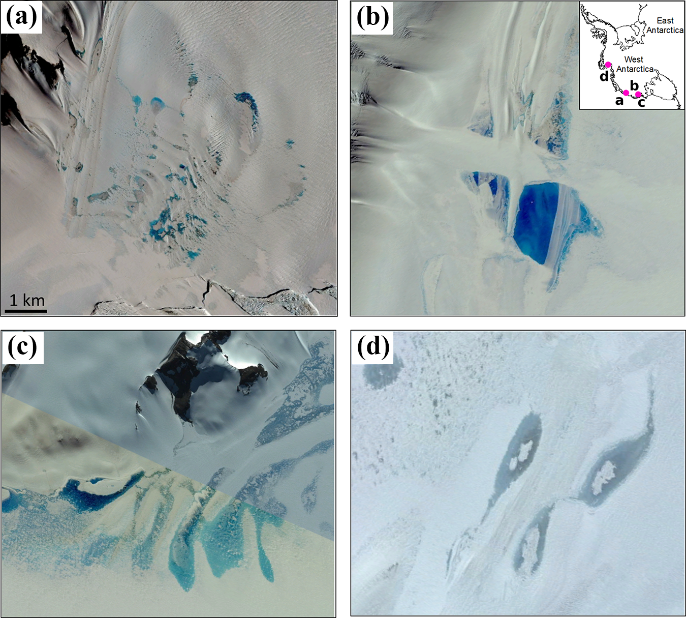
Examples of supraglacial lakes on the West Antarctic Ice Sheet visible in Digital Globe (Google Earth) imagery. (a) Hull Glacier (20th January 2015), (b) Sulzberger Ice Shelf (18th January 2013), (c) Sulzberger Ice Shelf (18th January 2013), (d) 45km east of Pine Island Glacier (13th February 2012), where lakes are likely to be refrozen at the surface. Scale bar applies to all four panels. Map data: Google, Maxar Technologies.
The first remote sensing assessment to draw attention to the widespread occurrence of SGLs in East Antarctica documented surface meltwater systems (lakes and channels) persistently forming on ice shelves around its periphery over multiple decades (Kingslake et al., 2017). This study found half of these drainage systems originate within 3.6km of blue ice and within 8km of exposed rock (Kingslake et al., 2017). This association could explain why SGLs typically extend further inland (up to 500km) at higher elevations (> 1000m) than those on Antarctic Peninsula ice shelves (Table 3). Indeed, SGLs have been recorded within 600km of the South Pole, on Shackleton Glacier, adjacent to exposed rock and moraine at the glacier margins (Kingslake et al., 2017). A more recent and comprehensive assessment recorded over 65,000 SGLs during January 2017, around the peak of the melt season (Stokes et al., 2019). This assessment recorded high lake densities (>0.08km2 SGL area per 1km2) in Wilkes Land, Queen Mary Land, Mac. Roberston Land, Enderby Land and Dronning Maud Land, as well as in previously undocumented regions such as Kemp Land, Terre Adélie and George V Land. Lakes were found to preferentially form near grounding lines on floating, low-elevation and slow-moving (<120m a-1) ice, supporting previous analysis (Section II; Kingslake et al., 2017).
The locations of lakes around the East Antarctic margin are strongly controlled by regional-scale wind patterns and locally enhanced ablation (Kingslake et al., 2017; Lenaerts et al., 2017). Katabatic winds, more persistent than sporadic föhn events on Larsen B, induce vertical mixing, which locally increases near-surface air temperatures. Surface melt is enhanced by these winds scouring snow/firn and exposing albedo-lowering blue ice, leading to meltwater ponding (Lenaerts et al., 2017a). Consequently, SGLs are often clustered around and immediately downstream of ice shelf grounding zones on the EAIS, proximal to these low-albedo areas and where surface slopes decrease (Kingslake et al., 2017; Lenaerts et al., 2017; Stokes et al., 2019; Winther et al., 1996).
It has also been shown that SGLs are persistent features of East Antarctic ice shelves across decadal timescales (Bell et al., 2017; Kingslake et al., 2017). The Amery Ice Shelf is a prominent example, where SGLs have regularly formed in longitudinal foliations and crevasses since at least 1974 across low-lying coastal regions, the largest reaching ∼80km in length (Hambrey and Dowdeswell, 1994; Kingslake et al., 2017; Mellor and McKinnon, 1960; Moussavi et al., 2020; Phillips, 1998; Stokes et al., 2019; Swithinbank, 1988). Ice dolines on some of these ice shelves (Amery and Roi Baudouin) are larger and deeper than those reported on Larsen B Ice Shelf, which suggests englacial drainage of SGLs (Bindschadler et al., 2002; Fricker et al., 2002; Lenaerts et al., 2017; Mellor and McKinnon, 1960) (Table 3). Observations of in-situ lake disappearance on Langhovde Glacier floating tongue in Dronning Maud Land in as little as five days also suggests that SGLs are likely to be draining englacially (Figure 11) (Langley et al., 2016). Given that lake volumes on several ice shelves (e.g. Amery, Riiser-Larsen, Shackleton and Moscow University) are estimated to exceed the average lake volume on Larsen B prior to its collapse (Glasser and Scambos, 2008; Stokes et al., 2019), lakes could be draining rapidly on some East Antarctic ice shelves and making them vulnerable to collapse. Whether ice shelf hydrofracturing occurs, however, is governed not only by meltwater distribution and volume stored in SGLs but also by stress conditions within the ice shelf (Alley et al., 2018; Christoffersen et al., 2018; Fürst et al., 2016). For example, the likelihood of some ice shelves (e.g. Amery) undergoing lake hydrofracture-driven collapse is low, owing to their thickness and large-scale geometry, which controls the stress regime and confines them to a narrow embayment with multiple topographic pinning points (Alley et al., 2018; Fürst et al., 2016; Stokes et al., 2019).
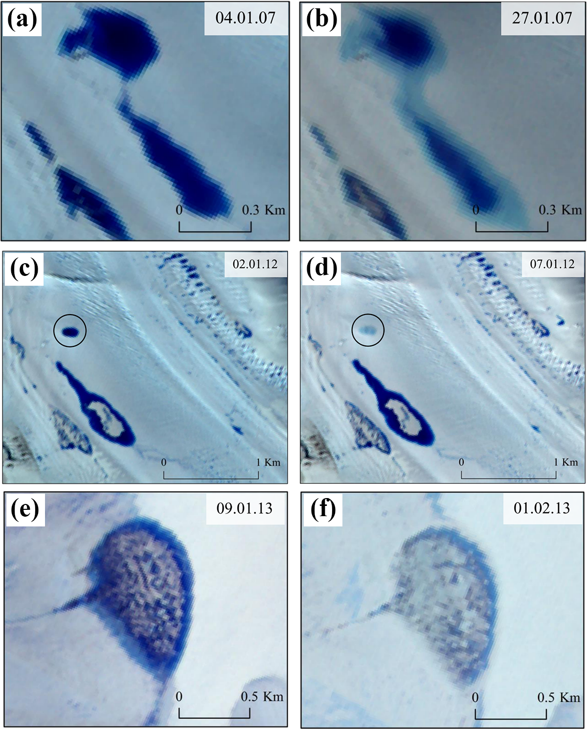
(a) and (b): SGL shrinking on the floating tongue of Langhovde Glacier, Dronning Maud Land, during January 2007. (c) and (d): SGL disappearance in five days on the floating tongue. (e) and (f): SGL refreezing in February 2013 at the end of the austral summer melt season as surface air temperatures decline (reproduced from Langley et al., 2016).
The vulnerability of East Antarctic ice shelves to future melt-induced hydrofracture could be modulated by the export of surface meltwater across ice shelf surfaces (Bell et al., 2017). Meltwater ponds tens of kilometres in area and several metres deep on the Nansen Ice Shelf are drained by an interconnected network of streams and shear-margin rivers, terminating in a 130 m-wide waterfall, which evolves as melt increases during warmer melt seasons (Bell et al., 2017). The likelihood of meltwater-induced fracturing can also be limited if flexure is not sufficiently widespread to affect other lakes (Banwell et al., 2019). This is the case on McMurdo Ice Shelf (MIS), which flexes by up to 1 m over weekly timescales at the centre of lakes that have filled to ∼2m depth and which are then drained by slow overflow (Banwell et al., 2019; MacAyeal et al., 2020).
4.3 Summary
The spatial distribution of SGLs in Antarctica reflects the complex interplay between localised and regional melt-enhancing processes, including katabatic wind-induced mixing and snow scouring, low-albedo nunataks and blue ice, together with firn air content (Datta et al., 2019; Kingslake et al., 2017; Lenaerts et al., 2017; Stokes et al., 2019). Our review indicates that on the Antarctic Peninsula, lakes were present on several ice shelves prior to their disintegration, and currently form on several of the largest remaining ice shelves. In East Antarctica, SGLs are persistent features of ice shelf grounding zones, driven by katabatic winds and locally enhanced ablation. Elsewhere around the margin of Antarctica there remain regions where SGLs have not yet been reported in the scientific literature, notably most of West Antarctica. SGLs are likely to become more numerous on firn-depleted ice shelves, and perhaps the lower reaches of other outlet glaciers that experience prolonged and excessive melting (Lenaerts et al., 2016; Rintoul et al., 2018) and more frequent föhn winds (Datta et al., 2019; Wiesenekker et al., 2018).
V Future challenges and opportunities
Based on our review, and in comparison to observations from the GrIS, it is clear that there remains much to be done in terms of understanding the controls on SGL distribution and evolution in Antarctica (cf. Bell et al., 2018). This includes the controls on lake occurrence in Antarctica, the evolution of SGLs through melt seasons and the vulnerability of ice shelves to SGL-induced collapse. These issues are now discussed as a series of key questions, several of which touch on some key priorities identified in the Scientific Committee on Antarctic Research (SCAR) Horizon Scan, such as the impact of changes in surface melt evolution over ice shelves and the Antarctic ice sheet (Kennicutt et al., 2014).
5.1 What are the controls on lake occurrence in Antarctica?
Although recent pan-ice sheet assessments have improved our understanding of the broad-scale climatic and ice surface controls on SGL formation (Kingslake et al., 2017; Lenaerts et al., 2016; Stokes et al., 2019), there remains a need to understand more precisely the links between near-surface climatic conditions and lake development. It is known that surface melt is poorly simulated by regional climate models in regions where SGLs tend to form, for example near grounding zones (Kingslake et al., 2019; Van Wessem et al., 2018). The complex interaction between ice surface characteristics and local-scale climatic controls, such as firn density, föhn or katabatic winds, ice surface albedo and topography, make it difficult to predict where SGLs may form based only on modelled surface melt (Stokes et al., 2019). The difficulty in resolving localised albedo-melt feedbacks is particularly acute with lower-resolution (27km) regional climate models, which tend to underestimate surface melt in areas of more complex topography. Lenaerts et al. (2018) found that a higher resolution (5.5km grid) version of the regional climate model RACMO2 was able to better resolve small-scale variability in climate, surface melt and surface mass balance caused by topography and thus reproduced surface melt more accurately over such areas. In this regard, it would be useful to generate runoff estimates from higher resolution regional climate model simulations and test the likelihood of different regions supporting SGLs under specific climatic thresholds and their effect on lake distributions and densities. Similarly, it would also be useful to explore the relative importance of climatic and glaciological controls in governing SGL formation in regions of Antarctica experiencing high surface melt and persistently occupied by SGLs, such as towards ice shelf calving fronts. This would be greatly aided, for example, by targeted field measurements of local variations in near-surface air temperature, snowfall and firn air content.
5.2 How do supraglacial lakes evolve through melt seasons in Antarctica?
SGL evolution during melt seasons remains poorly understood in Antarctica, particularly area, depth and volumetric changes on grounded and floating ice over weekly timescales. Understanding seasonal variability in SGLs and its relationship with surface climate conditions is important for constraining the magnitudes of surface meltwater storage potentially available to enter the englacial hydrological system through crevasses and moulins. Existing assessments of seasonal SGL evolution are sparse and focus on individual Antarctic outlet glaciers or ice shelves (Banwell et al., 2019; Bell et al., 2017; Langley et al., 2016; Moussavi et al., 2020), limited by the spatial resolution and return period of satellite imagery. Quantitative estimates of regional SGL change remain unknown. For example, what is the variability of total SGL surface area from year to year? How much do lakes expand and deepen through the course of a melt season, and how does this vary between floating and grounded ice?
A valuable next step would be to use automated methods at the catchment and regional scales to track individual lake locations, areas and volumes. This would enable quantification of lake changes and the number of lakes that drain rapidly, drain slowly or simply freeze over. Identifying which lakes may be at risk of rapidly draining will require analysis of lake drainage distributions alongside climatic (near-surface air temperature), glaciological (ice surface elevation, slope, strain rate, ice-sheet thickness) and surface mass balance (melt, runoff) datasets to identify the conditions that may promote rapid drainage (Williamson et al., 2018). Time-series of lake depths and volumes are also needed to constrain volume-dependent lake drainage thresholds in numerical models of lake behaviour (e.g. Banwell et al., 2015; Krawczynski et al., 2009). Recent efforts have begun to derive lake depth and volume time-series over some Antarctic ice shelves, which have clear potential to generate continent-wide maps of lake occurrence and evolution (Moussavi et al., 2020). Comparisons between SGL characteristics (geometry, depth, volume) and SGL changes (including timings of lake initiation and drainage onset, and peaks in total stored SGL meltwater) in different regions of Antarctica and Greenland are much needed. This would be valuable for identifying lakes that are likely to drain englacially, potentially over rapid timescales (Banwell et al., 2014; Kingslake et al., 2019; Stokes et al., 2019). SAR imagery has so far been under-used in Antarctica to monitor SGLs, and could usefully be applied with optical imagery such as Sentinel-2 and/or Landsat-8 to more accurately detect lake refreezing into the snow/firn pack and overcome cloud cover obscuration (e.g. Miles et al., 2017).
Future pan-ice sheet inventories of SGLs in Antarctica should cover multiple melt seasons, which will enable us to see whether SGLs are appearing at higher elevations in regions experiencing atmospheric warming, as has been observed on Greenland (Howat et al., 2013). An inland expansion of SGLs has important implications for ice dynamics because these lakes could deliver meltwater to the ice sheet bed where the subglacial hydrological system is inefficient. This could lubricate the ice-bed interface and accelerate ice flow (Bell et al., 2018; Leeson et al., 2015).
It is known that SGL drainage on the Antarctic Peninsula can accelerate grounded ice flow, both indirectly (Scambos et al., 2004) and directly (Tuckett et al., 2019). Whether SGL drainage impacts the behaviour of grounded ice by draining to the bed and influencing dynamics at the ice–bed interface in West and East Antarctica remains unknown. In order to capture the behaviour and processes preceding, during and following individual SGL drainage events, low-cost autonomous sensors could be deployed with GPS, water pressure transducers, seismometers and thermistors to obtain in-situ measurements of ice surface flexure, water depth, seismicity and surface melt. This would capture whether peaks in meltwater discharge, ice displacement and uplift can be directly linked to lake drainage events and transient ice acceleration (Das et al., 2008; Doyle et al., 2013), and will enable us to make connections between local and regional changes in the supraglacial and subglacial hydrological systems.
5.3 Which ice shelves are vulnerable to supraglacial lake-induced collapse?
Another future priority is to better constrain the sensitivity of specific Antarctic ice shelves to lake-induced hydrofracturing. Is there, for example, a threshold density or volume of SGLs needed to induce widespread fracturing and disintegration for any given stress condition? How does this threshold vary between ice shelves and what processes preclude ice shelf collapse? This is especially important for ice shelves that may already be preconditioned for hydrofracture. In particular, this includes ice shelves with high annual surface melt rates, depleted firn air content and extensional stress regimes, and that lack topographic confinement and ‘passive’ ice, such as the Shackleton, West and Roi Baudouin ice shelves (Alley et al., 2018; Fürst et al., 2016; Kingslake et al., 2019). In contrast, it is important to identify the stress conditions or ice thickness of some ice shelves that means that they can support a large surface area of meltwater ponding without being vulnerable to hydrofracture-driven collapse.
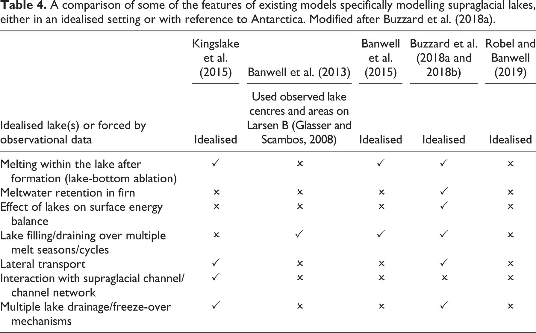
At present, challenges remain in being able to accurately represent hydrological and ice dynamic processes in models of SGL behaviour, such as hydrofracture and ice shelf flexure (Kingslake et al., 2019). Regional- and continental-scale ice-sheet models do not currently incorporate processes of ice shelf flexure and lake filling/draining, which may fracture ice shelves sufficiently to cause partial or complete disintegration. This limits how well SGL–ice shelf interactions can be modelled, including how lakes may promote future ice shelf instability (Banwell et al., 2013; Buzzard et al., 2018b; Robel and Banwell, 2019). Table 4 compares the features of existing SGL models and highlights that some processes are better represented in some models than others. For example, models can simulate lake evolution over multiple melt seasons (Banwell et al., 2013, 2015; Buzzard et al., 2018a, 2018b). However, these have tended to consider lakes as closed basins, when in fact observations have shown them to interact as part of an active hydrological network (Bell et al., 2017; Kingslake et al., 2017; Langley et al., 2016). More observations of lake evolution and interactions between lakes will benefit the development of future ice shelf models with regard to modelling the future impacts of SGL formation on ice shelf calving and stability.
A comparison of some of the features of existing models specifically modelling supraglacial lakes, either in an idealised setting or with reference to Antarctica. Modified after Buzzard et al. (2018a).
In conjunction with ice shelves, the vulnerability of floating outlet glacier tongues to these processes warrants further investigation. Assessments should focus on whether lake growth and drainage on outlet glaciers may be linked to fracturing or calving of their floating tongues, perhaps associated with sea-ice ponding and break-out events. For example, in Wilkes Land, East Antarctica, SGLs may have contributed to landfast sea-ice weakening prior to its break-up, which was followed by simultaneous outlet glacier disintegration (Miles et al., 2017).
VI Conclusions
In this paper, we have reviewed how advances in optical and radar satellite remote sensing have rapidly improved our knowledge of Antarctic SGLs in the last few decades. Recent increases in satellite sensor spatial resolution and revisit times have revealed that SGLs are forming around most marginal areas of the ice masses in Antarctica. From our review, it is clear that we now have a detailed knowledge of the broad-scale ice surface and climatic conditions associated with lake formation. Ice surface depressions dictate where SGLs form on the ice sheet surface, with lake formation dependent on near-surface firn air content and controlled by localised and regional wind patterns and locally enhanced ablation. These factors combine to produce the highest densities of lakes in the upper reaches of ice shelves and clustered down-ice of grounding zones. We are now able to exploit the major advances in the spatial and temporal resolution of several satellite sensors to map SGL extent, depth and volume using semi-automated methods over the whole continent. This has resulted in new knowledge of lake distributions and drainage mechanisms in some regions, perhaps with the exception of the West Antarctic Ice Sheet (WAIS).
In relation to ice dynamics, observations show that SGLs occupy most Antarctic Peninsula ice shelves and can be important precursors to crevasse hydrofracturing and ice shelf collapse. In East Antarctica, lakes persistently occupy ice shelves and may be draining through the ice, but ice shelf vulnerability to hydrofracture could be lower owing to geometric controls on stress conditions and meltwater export from ice shelf surfaces. However, our knowledge of SGL evolution within and between melt seasons remains limited, together with the influence of near-surface climate on SGL occurrence and the sensitivities of remaining Antarctic ice shelves to lake-induced collapse. Future research should quantify changes in lake distributions, volumes and drainage patterns at regional and ice sheet-scales to better understand the links between patterns of SGL behaviour and glacier and ice shelf stability, in particular by adopting a multi-sensor approach that exploits the increasing wealth of high-resolution satellite imagery. Further work could constrain critical ponding thresholds on remaining Antarctic ice shelves before critical meltwater-induced disintegration is triggered. This is urgently required to better predict the role of SGLs in future Antarctic ice mass loss.
Footnotes
Acknowledgements
JFA acknowledges a Natural Environment Research Council Doctoral Training Partnership Studentship (grant no. NE/L002590/1). We acknowledge the Norwegian Polar Institute’s Quantarctica package. The authors are grateful for comments during the peer review process and also thank the Editor.
Author contributions
JFA, CRS and SSRJ conceived the idea for the manuscript. JFA led the preparation and writing of the manuscript, with all authors contributing ideas and editing. JFA produced the figures.
Data availability
Satellite imagery was sourced from the United States Geological Survey EarthExplorer (https://earthexplorer.usgs.gov/), National Snow and Ice Data Center Antarctic Ice Shelf Image Archive (http://nsidc.org/data/iceshelves_images/), Google Earth, and the DigitalGlobe image viewer (![]() ).
).
Declaration of conflicting interests
The author(s) declared no potential conflicts of interest with respect to the research, authorship, and/or publication of this article.
Funding
The author(s) disclosed receipt of the following financial support for the research, authorship, and/or publication of this article: JFA acknowledges a Natural Environment Research Council Doctoral Training Partnership Studentship (grant no. NE/L002590/1).