
Abstract
Unsustainable exploitation of groundwater in northwestern India has led to extreme but spatially variable depletion of the alluvial aquifer system in the region. Mitigation and management of groundwater resources require an understanding of the drivers behind the pattern and magnitude of groundwater depletion, but a regional perspective on these drivers has been lacking. The objectives of this study are to (1) understand the extent to which the observed pattern of groundwater level change can be explained by the drivers of precipitation, potential evapotranspiration, abstraction, and canal irrigation, and (2) understand how the impacts of these drivers may vary depending on the underlying geological heterogeneity of the system. We used a transfer function-noise (TFN) time series approach to quantify the effect of the various driver components in the period 1974–2010, based on predefined impulse response functions (θ). The dynamic response to abstraction, summarized by the zeroth moment of the response M0, is spatially variable but is generally large across the proximal and middle parts of the study area, particularly where abstraction is high but alluvial aquifer bodies are less abundant. In contrast, the precipitation response is rapid and fairly uniform across the study area. At larger distances from the Himalayan front, observed groundwater level rise can be explained predominantly by canal irrigation. We conclude that the geological heterogeneity of the aquifer system, which is imposed by the geomorphic setting, affects the response of the aquifer system to the imposed drivers. This heterogeneity thus provides a useful framework that can guide mitigation efforts; for example, efforts to decrease abstraction rates should be focused on areas with thinner and less abundant aquifer bodies.
Keywords
I Introduction
In regions with large aquifer systems that undergo frequent water stress, groundwater is often used as an additional water source. If groundwater abstraction exceeds the natural groundwater recharge over an area for long periods of time, over-exploitation or persistent groundwater depletion occurs (Wada et al., 2010). The unsustainable exploitation of groundwater resources is now a very significant problem globally and requires urgent attention (Aeschbach-Hertig and Gleeson, 2012; Gleeson et al., 2010). As Famiglietti (2014) describes, whilst groundwater is a critically important global water resource, it is given insufficient attention within management systems compared to visible surface water resources. This is particularly true in countries where water governance is weak or absent and monitoring of aquifers is inadequate. Consequently, for many heavily exploited aquifers there is a lack of knowledge about (1) how groundwater storage responds to various drivers, such as precipitation, evapotranspiration, abstraction and irrigation, (2) how storage variations relate to aquifer heterogeneity, and (3) how future changes in groundwater levels might be anticipated and mitigated on the basis of these various drivers. Such knowledge is critical for management, especially if the heterogeneity of the aquifer system leads to substantially different responses to future stresses in different parts of a region.
The Indo-Gangetic foreland basin is one of the world’s most prominent hotspots of groundwater depletion, especially in northwestern India (Chen et al., 2014; Kumar et al., 2006; MacDonald et al., 2016; Richey et al., 2015; Rodell et al., 2009; Shah, 2009; Tiwari et al., 2009). This has been caused by the increased use of groundwater for irrigation since the mid-1960s as part of the “Green Revolution,” the popular name for the agricultural strategy that aimed to make India self-sufficient in food grain production. Groundwater abstraction for irrigation has become a particularly severe issue in the states of Punjab and Haryana, whose contribution to national food grain production increased from 3% before the Green Revolution to approximately 20% at the end of the 20th century (Singh, 2000). Rapid groundwater level decline associated with groundwater pumping has been documented across these states by MacDonald et al. (2016). However, in parts of the region, significant groundwater level rise has also occurred due to infiltration from canal irrigation return flow and canal seepage (Joshi et al., 2018). Recent work by Asoka et al. (2017) showed that groundwater storage changes in northwestern India between 2002 and 2013 can be explained by both abstraction and precipitation, although the former appears to have been somewhat more important. They considered only a single time series of storage change, however, and did not assess spatial variations in either groundwater level changes or in the potential drivers of those changes.
Here we address the urgent societal issue of groundwater depletion in northwestern India by applying a time series analysis to understand the spatial variation in groundwater level change, focusing in particular on the area between the Sutlej and Yamuna Rivers where historical decline has been greatest. The objectives of this study are to: (1) assess whether a time series model using parsimonious, physically-related impulse-response functions can reproduce changes in the spatial pattern of groundwater levels since 1974; (2) understand the extent to which the observed pattern of groundwater level change can be explained by the drivers of precipitation, potential evapotranspiration (PET), abstraction, and canal irrigation; and (3) investigate the extent to which the impacts of these drivers depend on the geological heterogeneity of the aquifer system. First, we present the available climatic and groundwater level data for the region, and describe the time series model and its implementation. We examine the influence of individual driver components on the aquifer system over time, and then use a single measure of the system response to quantify spatial variations in response across the study area. Finally, we relate our results to the geological framework of the study area, and explore the potential implications of the results for groundwater management and their application to other depleting aquifer systems.
II Study area
This study focuses on the northwestern region of India, which is part of the Indo-Gangetic foreland basin and is fed by the Sutlej River in the west and the Yamuna River in the east of the study area (Figure 1(a)). Recent studies have identified sediment deposits in the study area that were sourced from the Yamuna and Sutlej catchments (Clift et al., 2012; Singh et al., 2017), and geophysical profiles have verified the existence of large paleochannels within the subsurface (Khan and Sinha, 2019; Sinha et al., 2013). The alluvial aquifers in this study area are formed by sediments eroded from the Himalaya and redistributed by the Sutlej and Yamuna rivers, forming two major sedimentary fan systems (Geddes, 1960; Singh et al., 2016; Van Dijk et al., 2016a). The distribution of the channel sand deposits that form the primary aquifer bodies within these fan systems is controlled by river avulsion, sedimentation rate, and the stacking pattern of fluvial channel-belt units (Allen, 1978, 1984; Bridge, 1993; Bridge and Leeder, 1979; Heller and Paola, 1996; Holbrook, 2001; Leeder, 1978; Sheets et al., 2002; Straub et al., 2009; Van Dijk et al., 2016b). This alluvial stratigraphy, in turn, determines the characteristics and productivity of the aquifer (Anderson, 1989; Fogg, 1986; Weissmann et al., 1999), in terms of (1) the percentage of sand-rich aquifer bodies in the subsurface; (2) the geometry and dimensions of the aquifer bodies; (3) their hydraulic conductivity and specific yield; and (4) their vertical and horizontal connectivity (Flood and Hampson, 2015; Larue and Hovadik, 2006; Renard and Allard, 2013).
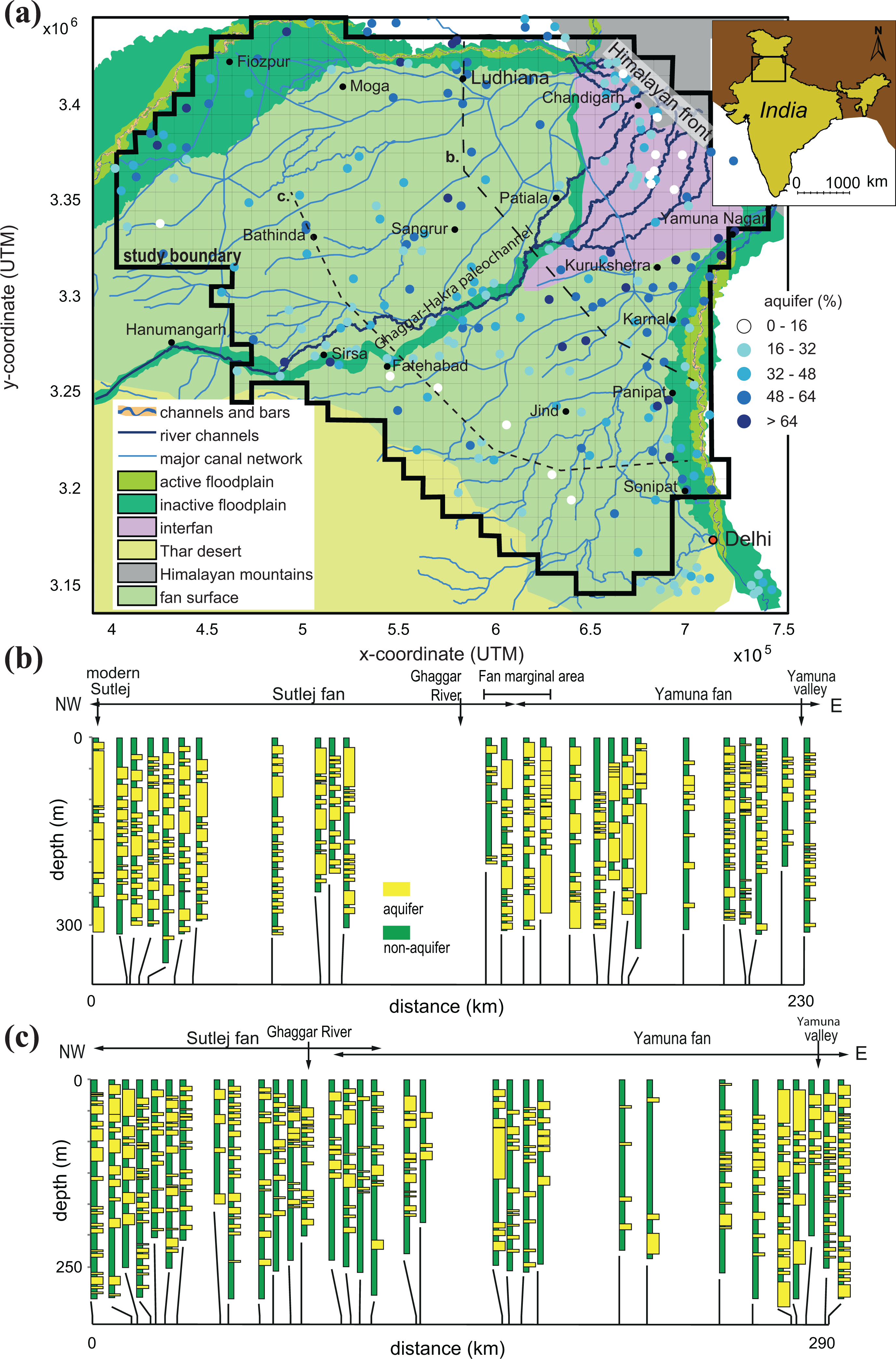
(a) Geomorphological map and the subsurface aquifer percentage of the study area in northwestern India, modified after Van Dijk et al. (2016a). The study area covers the Sutlej and Yamuna fans (light green) and the interfan area between them (pink). Dark green areas show the incised valleys of the modern Sutlej and Yamuna rivers and the Ghaggar–Hakra paleochannel (Singh et al., 2017). Light blue lines show major canals. Dots show bulk aquifer percentage in the upper 200 m of the subsurface, based on CGWB aquifer-thickness logs (see Van Dijk et al., 2016a for description). Long-dashed line shows the medial transect in (b), while the short-dashed line shows the distal transect in (c). The study area is outlined by the thick black line and divided into 10 x 10 km grid cells. (b) Medial transect illustrating aquifer (yellow) and non-aquifer (green) units in the subsurface. Note abundant stacked aquifer bodies. (c) Distal transect showing the lower abundance of aquifer bodies compared to the medial part of the fan. Transects in panels (b) and (c) modified from Van Dijk et al. (2016a).
Van Dijk et al. (2016a) established that aquifer body thickness and percentage vary in systematic and predictable ways between proximal and distal parts of the fan systems, and between the fans and the interfan or marginal areas between them (Figure 1(a)). The elongated channel deposits that form aquifer bodies are highly connected in the down-fan direction but are less connected in the lateral direction. The bulk percentage of aquifer bodies decreases in the down-fan direction (Figure 1(b) and (c)), although the distribution of aquifer-body thickness remains the same (Van Dijk et al., 2016a). The geomorphic distinction between fan and interfan settings within the Indo-Gangetic basin also introduces an important large scale lateral heterogeneity. Aquifer bodies are generally thinner and less abundant for the interfan area, whereas the fans consist of abundant stacked channel sand bodies as result of the formation and subsequent filling of incised valleys across the fan surface (Van Dijk et al., 2016a). An example of subsequent filling of an incised valley is the Ghaggar–Hakra paleochannel (Singh et al., 2017), which is at the border of the Sutlej and Yamuna fan system. Thus, the observations provide evidence that the alluvial aquifers in northwestern India are highly spatially heterogeneous, and that the surface geomorphology provides a clear guide to the subsurface architecture of the alluvial aquifer system. Van Dijk et al. (2016b) further argued that the geological framework imposed by these fan systems and the interfan areas should be used as a basis for understanding and relating aquifer properties, groundwater level changes, and potential groundwater management approaches.
3 Methods
1 Methodology
Here, we focus on trying to understand the relative role of different drivers, imposed on the heterogeneous regional framework mentioned above, in explaining the rates and patterns of historical groundwater level change. This requires a groundwater modeling approach. A diverse range of models have been applied to simulate groundwater dynamics, and the appropriate degree of model complexity depends on the goal of the modeling, the amount of data with which to constrain the model, and practical project constraints (Guthke, 2017). Distributed groundwater models, which solve physical laws governing groundwater flow by discretizing the aquifer domain, remain the most widely used. This approach allows for complex heterogeneous and anisotropic fields of aquifer properties, but typically results in models with large numbers of parameters, for which a careful assessment of uncertainty is required (Hill and Tideman, 2007; Refsgaard et al., 2012; Rojas et al., 2010). Given the poor spatial resolution across northwestern India in both measurements of aquifer properties (UNDP, 1985; Van Dijk et al., 2016a) and water levels (MacDonald et al., 2016), it is difficult to justify the use of such a complex approach in this region.
Conceptual, lumped-parameter modeling is an alternative approach that simplifies the representation of processes incorporated in physically-based models, but maintains some fundamental physical principles from our conceptual understanding of groundwater systems (e.g. Kazumba et al., 2008; Mackay et al., 2014; Park and Parker, 2008). These models incorporate parameters that can be associated with measurements of properties made in the field, such as hydraulic conductivity or specific yield. For example, Mackay et al. (2014) applied a lumped-parameter groundwater model, AquiMod, to simulate groundwater levels in observation boreholes in different aquifers across the UK. The model was driven by rainfall and PET time-series, and contained three conceptual stores representing soil, an unsaturated zone, and a saturated aquifer, which were used to simulate infiltration to the groundwater table. As with other lumped-parameter groundwater models (Barrett and Charbeneau, 1997; Hong et al., 2017; Long, 2015; Pozdniakov and Shestakov, 1998), however, AquiMod typically required the specification of a large number of parameters, although many of these could be fixed based on prior information and expert judgment. Given the limited prior information for this region, there are no valid ways to constrain all of those parameters, and therefore we did not adopt this approach.
Another means of simulating groundwater level fluctuations is by the use of a statistical time series approach, such as transfer function-noise (TFN) models (Berendrecht et al., 2003; Von Asmuth et al., 2002), which are especially useful for modeling systems whose behavior cannot easily be described by physical processes or quantified by physically-observable parameters. TFN models have been widely used in hydrology and can be divided into three types: (a) models that start from a geo-statistical methodology, applying space-time kriging or co-kriging (Van Geer and Zuur 1997); (b) models that are based on multivariate time series analysis, where multiple time series are correlated in space (Von Asmuth et al. 2002); and (c) models that combine elements of methods (a) and (b) (Bierkens et al., 2001; Yuan et al., 2008). For example, Von Asmuth et al. (2008) used a time series analysis method to predict fluctuations in groundwater level from multiple drivers. They described a class of parsimonious TFN models that implement predefined impulse response functions in continuous time (PIRFICT), which circumvents a number of limitations of discrete TFN models linked to time discretization and model identification. The PIRFICT methodology has since been used in a number of studies to determine the effect of multiple drivers on groundwater levels in different regions of unconfined aquifers (Obergfell et al., 2013; Shapoori et al., 2015a). Application of the Von Asmuth et al. (2008) model is potentially useful for regions like northwestern India where (1) we lack a detailed physical understanding of the aquifer system and high-resolution subsurface data with which to constrain the key parameters (Van Dijk et al., 2016b), and (2) groundwater level is likely to be controlled by a small number of major driver components. This approach is ideal for understanding how groundwater responses vary spatially and how the response is linked to the underlying aquifer characteristics and geology. The model can approximate regional heterogeneity, but is not set up to deal with finer scale heterogeneity that is observed within individual channel bodies (Donselaar and Overeem, 2008; Holbrook, 2001; Miall, 1985; Van de Lageweg et al., 2016a, 2016b; Willis and Tang, 2010).
2 Data acquisition
For the model inputs we collected district-wise data on precipitation and PET from the Indian Meteorological Department (IMD) for the period 1951–2010. We obtained district-averaged abstraction values from the Central Groundwater Board (CGWB) for the years 2004, 2009, and 2011, and reconstructed the monthly groundwater abstraction for irrigation by the deficit between crop water requirements and effective precipitation. Groundwater level data were collected for the period 1974-2010 from borehole databases maintained by the state groundwater departments of Haryana and Punjab, and by the CGWB. Measurements were made twice yearly (pre- and post-monsoon) by the state groundwater departments, and four times yearly by the CGWB. For more detail on the data acquisition see the Supplemental Material.
Initial analysis of the climate and groundwater level data indicated a potential relation between groundwater level decline and total abstraction over the period of observations. This is not surprising (Asoka et al., 2017), although declines in groundwater level will be controlled by the amount by which abstraction exceeds groundwater recharge, rather than by the magnitude of abstraction itself. The analysis, and that by Asoka et al. (2017), does not illuminate the reasons for the spatial patterns in decline (Supplementary figure 3), however. In addition, the degree of scatter that is visible in Supplementary figure 4 suggests that abstraction alone is not an adequate predictor of groundwater level change. To investigate the response of groundwater levels to the combined effects of precipitation, PET, abstraction, and irrigation, we implemented a transfer function-noise time-series model.
3 Model setup
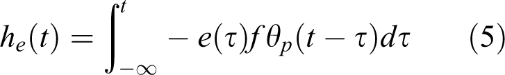
We adopted the formulation for multiple drivers presented by Von Asmuth et al. (2008) in the TFN method. This formulation relies on predefined impulse response functions for each driver in continuous time (Von Asmuth et al. 2002). The estimated groundwater level at time t in response to driver i,
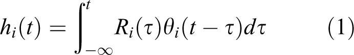
where

where
Equation (1) shows that impulse response functions must be defined for each of the drivers that we impose. Our impulse response function for precipitation,
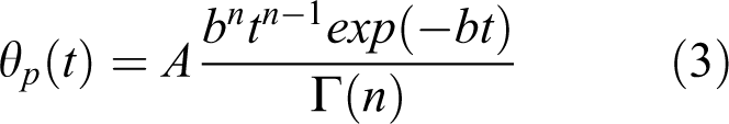
where A, b, and n are parameters that define the shape of
The physical interpretation of equation (3) is a series of coupled linear reservoirs where n is the number of reservoirs, b is the inverse of the reservoir constant normally used, and A adjusts the area of response (Von Asmuth et al., 2002). Von Asmuth et al. (2008) argued that PET should have a similar effect as precipitation on h, although it will have an opposite sign and a different magnitude. Consequently, water level in response to PET was modeled as
where e is the PET time series and
Earlier PIRFICT-based TFN modeling studies that incorporated groundwater abstraction (Obergfell et al., 2013; Shapoori et al., 2015a, 2015b; Von Asmuth et al., 2008) implemented a three-parameter impulse response function based on the Hantush (1956) solution to the drawdown in a leaky confined aquifer. Following Shapoori et al. (2015a, 2015b), we used a two-parameter impulse response function based on the Theis solution for the drawdown in a confined aquifer of the form
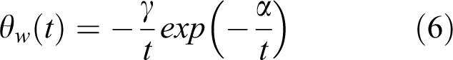
where α and γ are calibration parameters. The parameter γ is equivalent to
The final driver to be incorporated into the TFN model represents the combined effect of canal irrigation return flow and canal seepage. We modeled this response function with a simple exponential function of the form
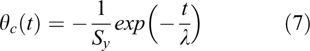
where
4 Model application
The TFN model was applied using a monthly time step to simulate the time series of cell-averaged groundwater levels independently for each of the 664 10 × 10 km cells across the study area. The drivers
Each model was run for the 60-year period 1951–2010, and calibrated against the 1974–2010 groundwater level time series. Therefore, the simulation period contains a 23-year spin up period, during which time the effect of pre-1951 memory in the impulse response functions is lost. The local drainage parameter, d, was fixed to a level defined by extrapolating the groundwater level data over the period 1974–1984 back to 1951 using linear regression. The model was calibrated using a Monte Carlo procedure, within which values for the eight parameters (A, b, n, f, γ, α, λ,
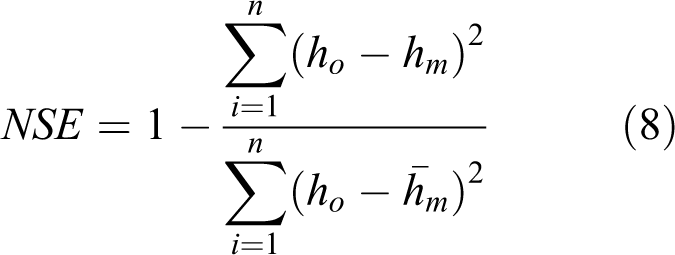
where
Ranges of parameter values sampled during Monte Carlo procedure.
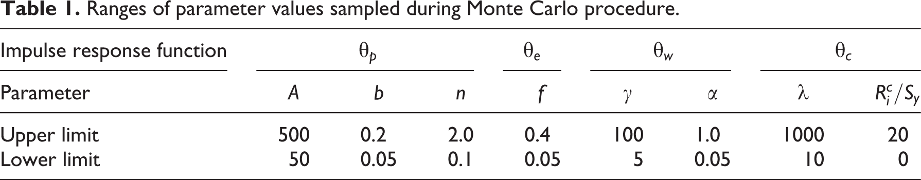
Parameter values for the impulse response functions were chosen to encompass a wide range of shapes and scales (Figure 2). An additional condition was imposed on the ratio
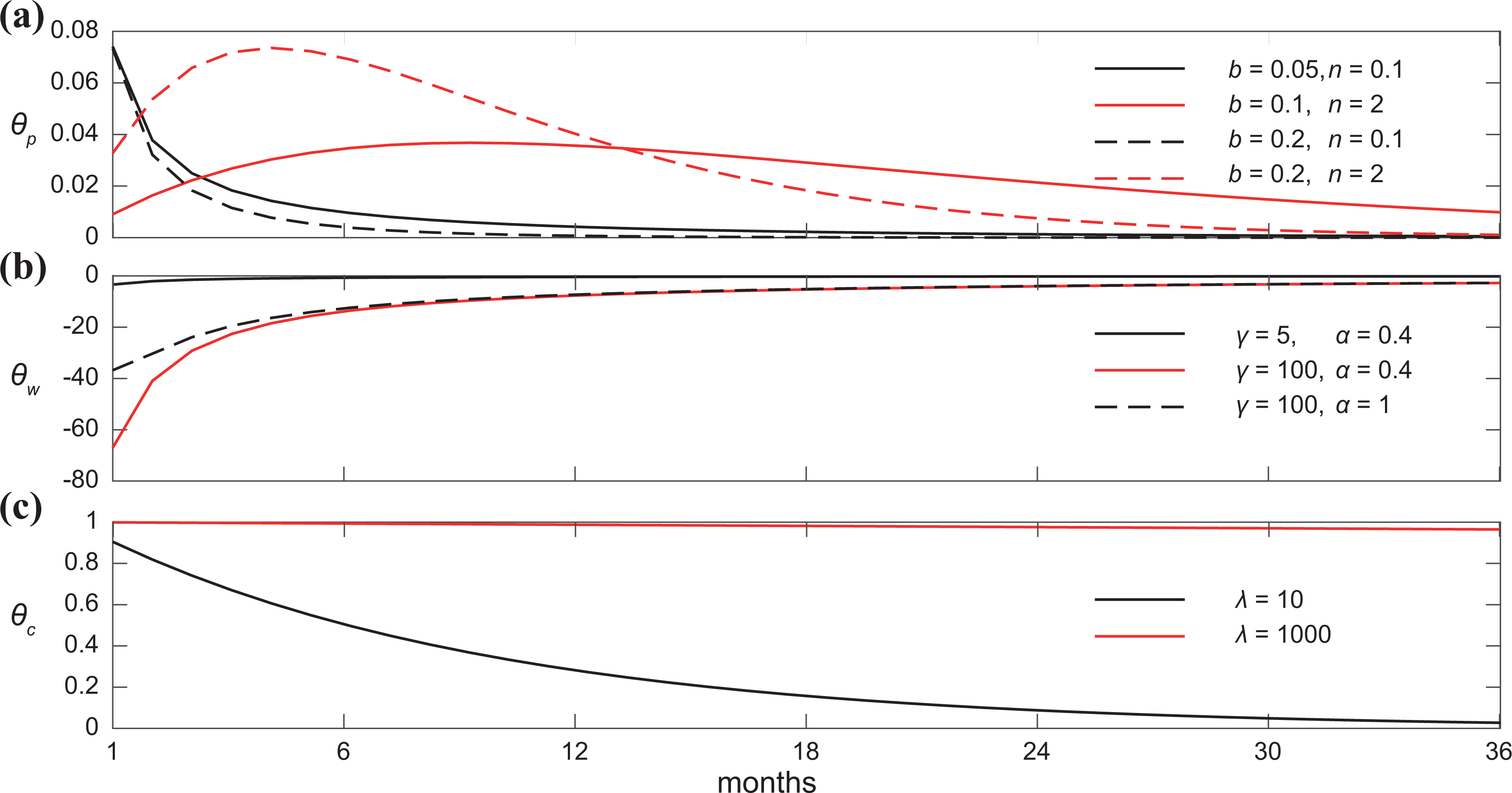
Example impulse response functions for (a) precipitation
5 Data analysis
A primary goal of this work is to assess not only the relative importance of different drivers in determining water level
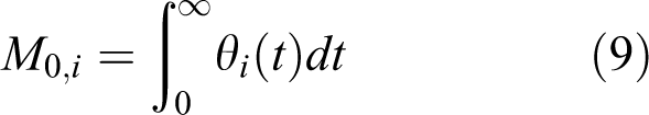
A large value of M0 means that the driver has a large effect on the groundwater level, due to a response that is large in magnitude, persistent in time, or both. A small value of M0 means that the effect on the groundwater level by the driver is minimal.
To characterize the spatial variation in the relative importance of precipitation, abstraction, and canal irrigation drivers, we plotted the zeroth moment for the best fit solution with the highest
IV Results
1 Groundwater level series
The measured groundwater level changes show a general groundwater level decline in the northeastern part of the study area and water level rise in the southwestern part over the period 1974–2010 (Figure 3(a)). The calibrated TFN model reproduces this overall pattern (Figure 3(b)). The model is able to capture the spatial distribution, although not necessarily the observed values, in areas of large groundwater level change. In detail, the modeled declines in groundwater level are more patchy than the observed pattern, and the absolute declines are somewhat under-predicted, leading to relatively high
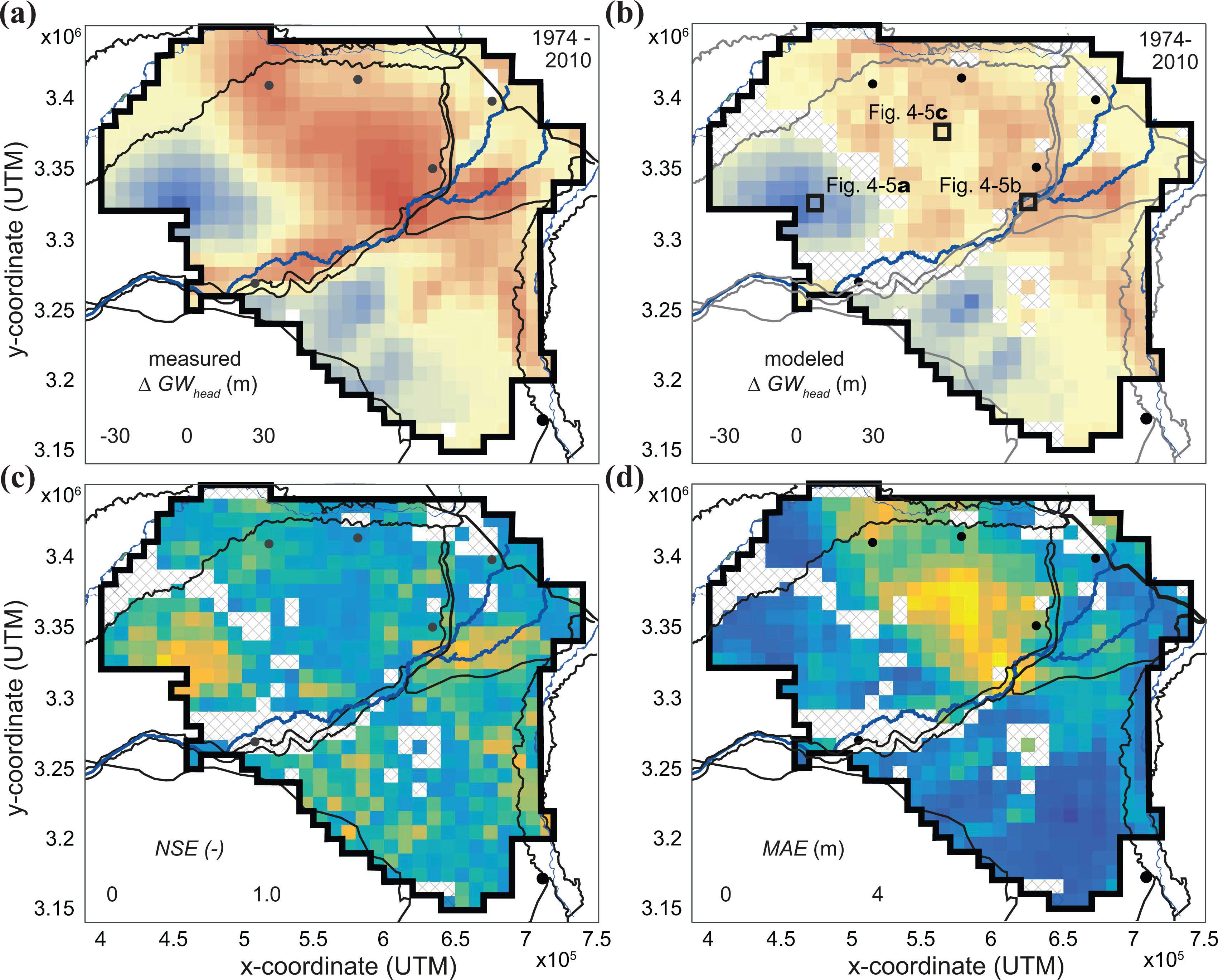
(a) Observed and (b) modeled groundwater level changes for the period 1974–2010. Black square boxes indicate grid cells that are elaborated in Figures 4 and 5. Cross-hatched cells yielded no model solutions with
We illustrate the results of the time series model from three example locations with different patterns of temporal evolution (see Figure 3(b) for locations): groundwater level rise, decline in the area of the Ghaggar–Hakra paleochannel, where we expect thinner and less abundant aquifer bodies (Van Dijk et al., 2016a), and decline on the Sutlej fan, where we expect thick and more abundant aquifer bodies (Figure 4). At each location, the modeled groundwater level is decomposed into four partial series to show the response of the level to precipitation, PET, abstraction, and canal irrigation. For the location with groundwater level rise (Figure 4(a)), the effect of canal irrigation on the groundwater level
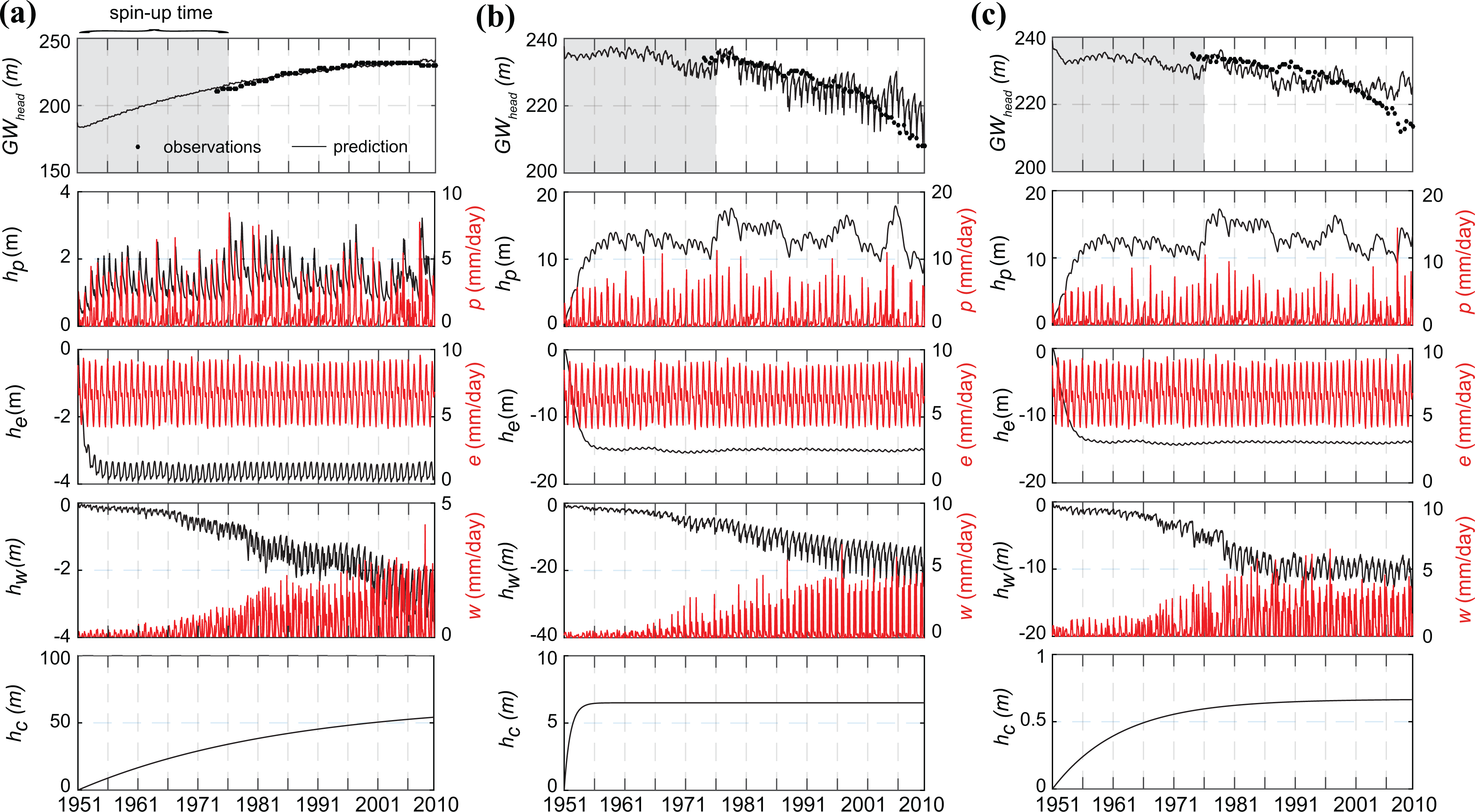
Three examples of TFN model outcomes for grid cells with (a) groundwater level rise, (b) groundwater level decline in the area of the Ghaggar–Hakra paleochannel, and (c) decline in the area of the Sutlej fan. See Figure 3 for locations. In each column, the top panel shows observed (dots) and predicted (black line) water levels over time; the gray area indicates the model spin-up time from 1951 to 1974. In the lower panels, the red lines indicate the input time series of precipitation, PET, and abstraction. Black lines indicate the contribution of each component to the water level. Groundwater level rise in (a) can be explained by the monotonically-increasing canal irrigation component (
Groundwater level decline in the area of the Ghaggar–Hakra paleochannel (Figure 4(b)) is dominated by the abstraction component
2 Impulse response functions
The impulse response function describes the dynamic response of the groundwater level after a sudden input or change of a driver i. The calibration parameters determine the shape of this response in terms of its amplitude and duration. In our implementation of the TFN model, impulse response functions are generated for each grid cell independently based on the water-level history and stresses imposed in that cell. Here we illustrate the best-fit impulse response functions for the same three locations that were shown in Figure 4. The response to precipitation is rapid for the location experiencing groundwater level rise (Figure 5(a)), but is delayed by a few months for the locations experiencing decline (Figure 5(b) and (c)). These relatively short-term responses explain why
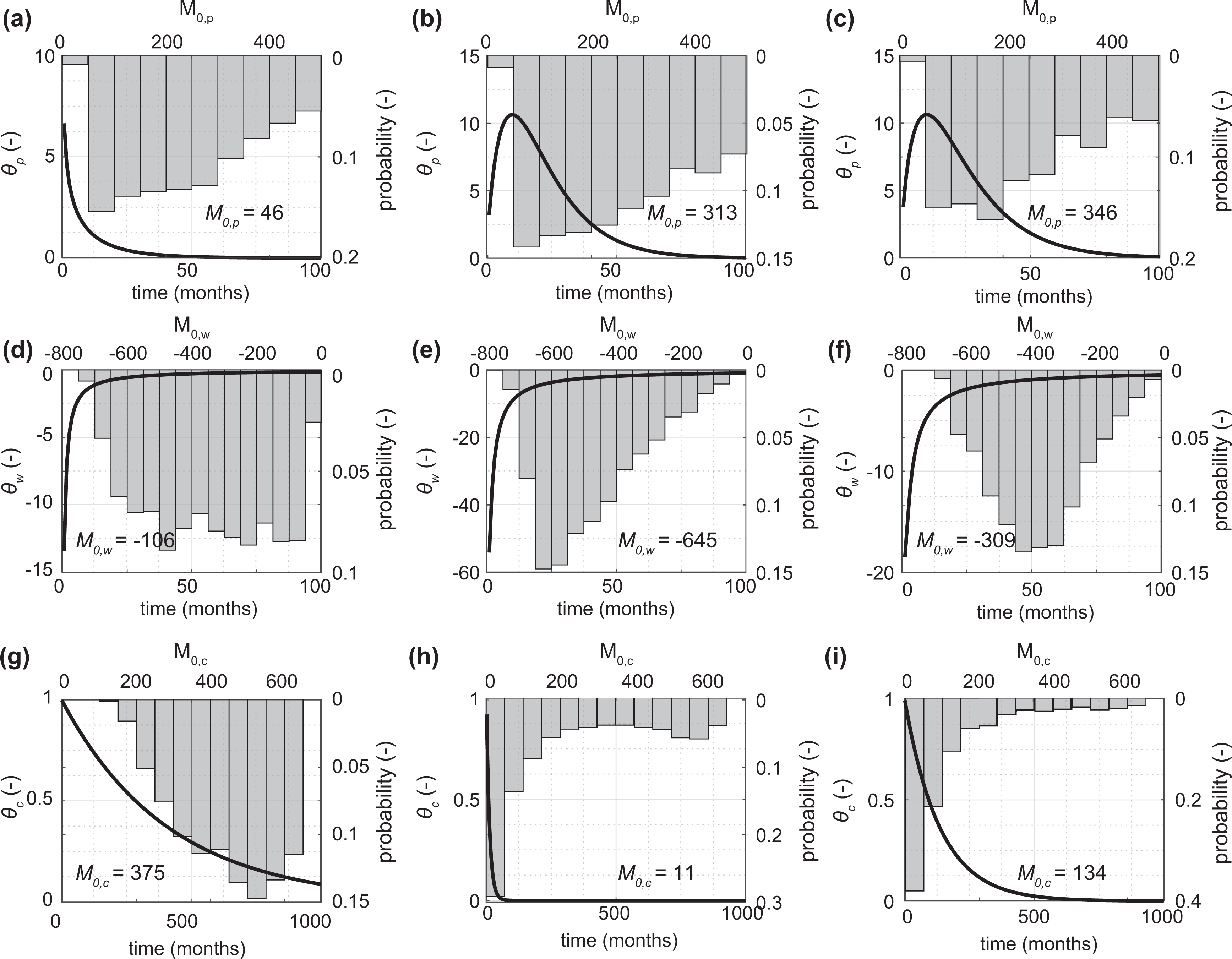
Best-fit impulse response functions, shown as black lines, for precipitation (top row), abstraction (middle row), and canal irrigation (bottom row) drivers for the three locations shown in Figure 3. The area under each response function curve gives the zeroth moment for precipitation (
There is substantial variability in M0 values for all three drivers, even when we consider only model outcomes with
3 Spatial variation of the zeroth moment
There are substantial and systematic variations in M0 for the precipitation, abstraction, and canal irrigation drivers across the study area (Figure 6). Recall that a high value of M0 means that the driver has a large influence on the groundwater level, and a low value means there is little influence. The response to precipitation is fairly uniform across the study area, except for a hotspot on the central part of the Sutlej fan (Figure 6(a) and (b)). This area has the highest
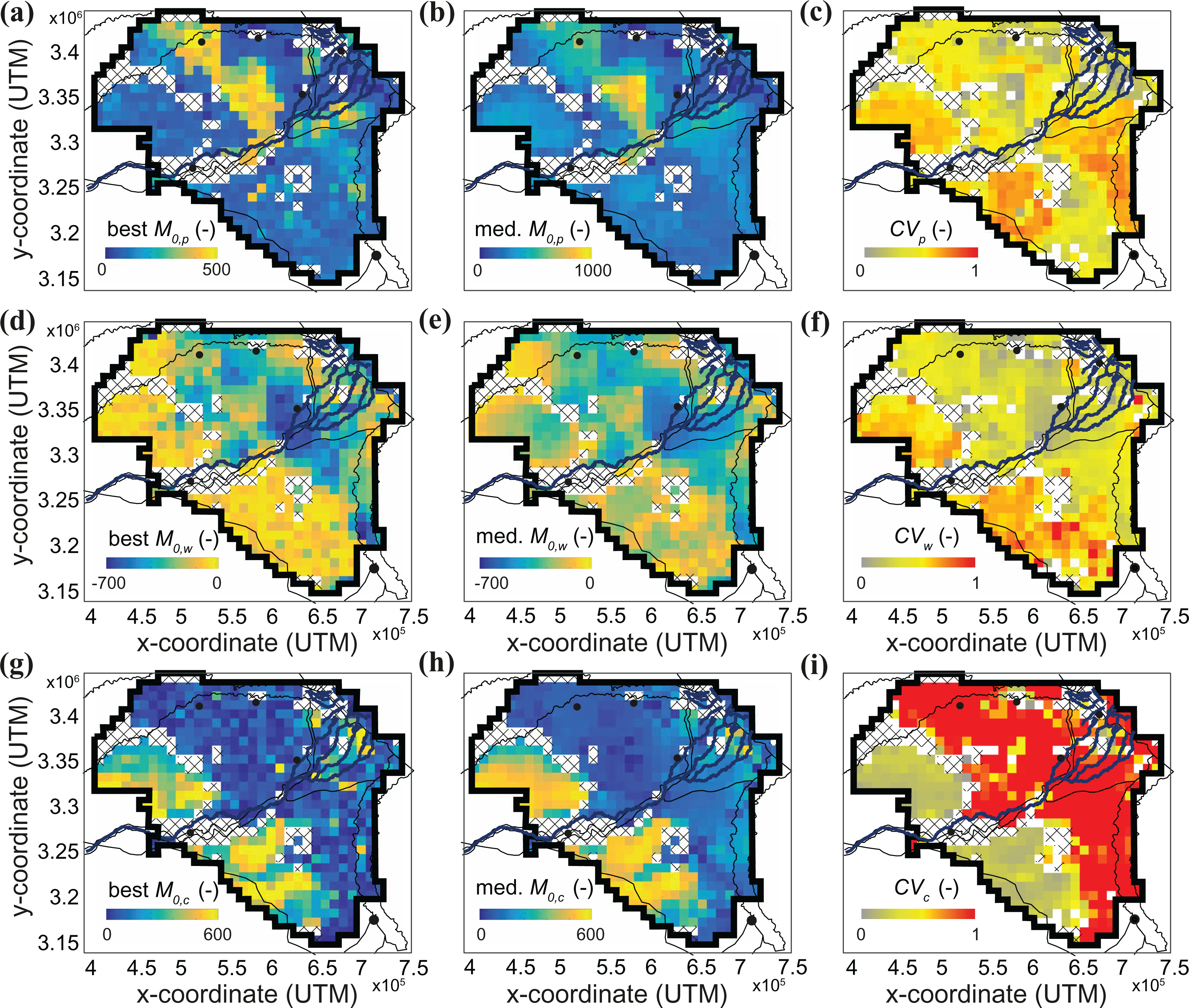
Spatial variation in the zeroth moment M0 of the impulse response functions for precipitation (top row), abstraction (middle row), and canal irrigation (bottom row) drivers. In each row, the left panel shows M0 for the best-fit model result in each grid cell, the middle panel shows the median M0 for all model runs with
The zeroth moment for the abstraction stress shows a strong negative response (Figure 6(d) and (e)) in the central part of the study area, and most notably in the interfan area between the Sutlej and Yamuna fans and along the Ghaggar–Hakra paleochannel (Figure 1). This high sensitivity to abstraction is visible in both best-fit and median model results, with a low coefficient of variation (Figure 6(f)), and is centered on the areas of greatest groundwater decline (Figure 3(a)). The distal parts of both fans show much lower sensitivity to abstraction, corresponding to lower overall groundwater depletion. Distal areas have some high values of the coefficient of variation; these areas have very small zeroth moments so the coefficient of variation is sensitive to small variations between model runs.
High values of the zeroth moment for canal irrigation
V Discussion
The TFN model yields insights into the response of groundwater levels to the four most common drivers that determine the groundwater depletion rate in northwestern India. Here we first discuss each individual parameter that sets the impulse response function and the zeroth moment of that response. Second, we link the spatial variation of the responses (as represented by the zeroth moment and the parameters) with the underlying geological heterogeneity in the aquifer system. Third, we discuss the implications of our model outcomes for understanding groundwater level changes, along with model limitations. Finally, we provide our recommendations for future sustainable groundwater management.
1 Link to specific drivers
Spatial variations in M0 are explained by the different parameters that determine θ, and so it is useful to examine the variations in those parameters for the median model solutions and their link to specific drivers. High values for
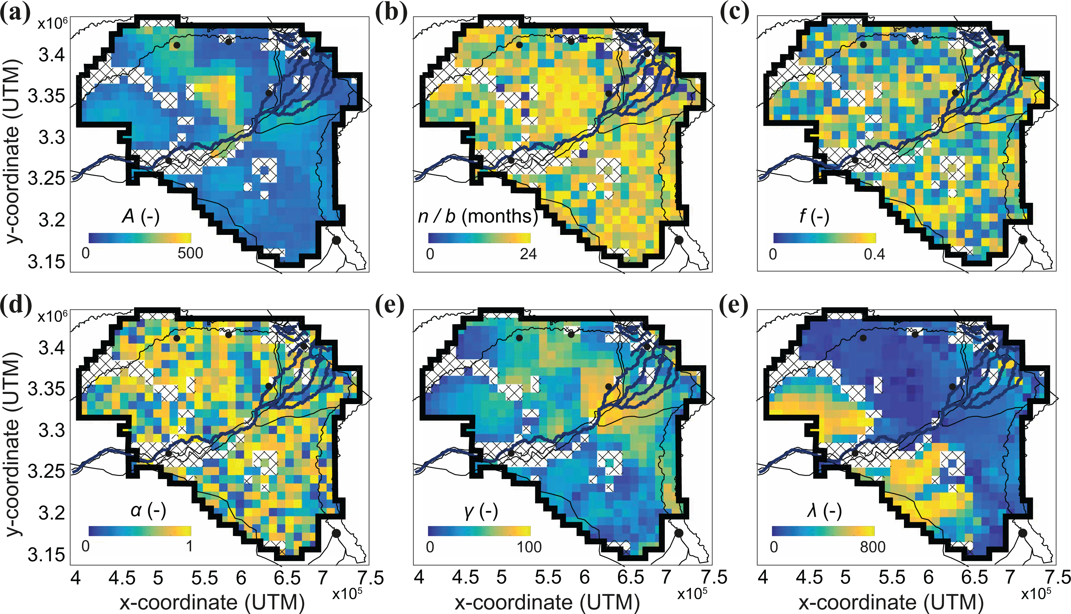
Model parameters associated with the median solution for all grid cells. (a) Parameter A is larger for the areas with groundwater level rise and especially for the central part of the Sutlej fan. (b) The ratio (
More interesting are the parameters that determine the variation of
2 Spatial relations between abstraction and geomorphology
The zeroth moment of the response to the abstraction driver
High levels of groundwater decline and high negative
3 Model implications and limitations
The time series approach was applied to study the spatial variation of groundwater level in response to multiple drivers for a regional hotspot of groundwater depletion in northwestern India. The model incorporated impulse response functions θ to four imposed drivers: precipitation, PET, abstraction, and canal irrigation. These response functions were calibrated against the observed groundwater levels to produce a cell-by-cell prediction of modeled groundwater levels through time. Supplementary figure 4 showed that there was only a weak relation between total abstraction or precipitation and the observed groundwater level changes on a cell-by-cell basis, irrespective of whether the level had risen or declined. The time series analysis demonstrates that there are strong spatial differences in the response to the four modeled drivers, as quantified by the zeroth moment M0 which is a stationary measure of the response to a driver. This, in turn, suggests that scaling the total abstraction or precipitation by M0 may improve the correlation between the total volumes and observed groundwater level change. However, when applying this to precipitation, a negative relation with groundwater level change is derived (Figure 8(a)).
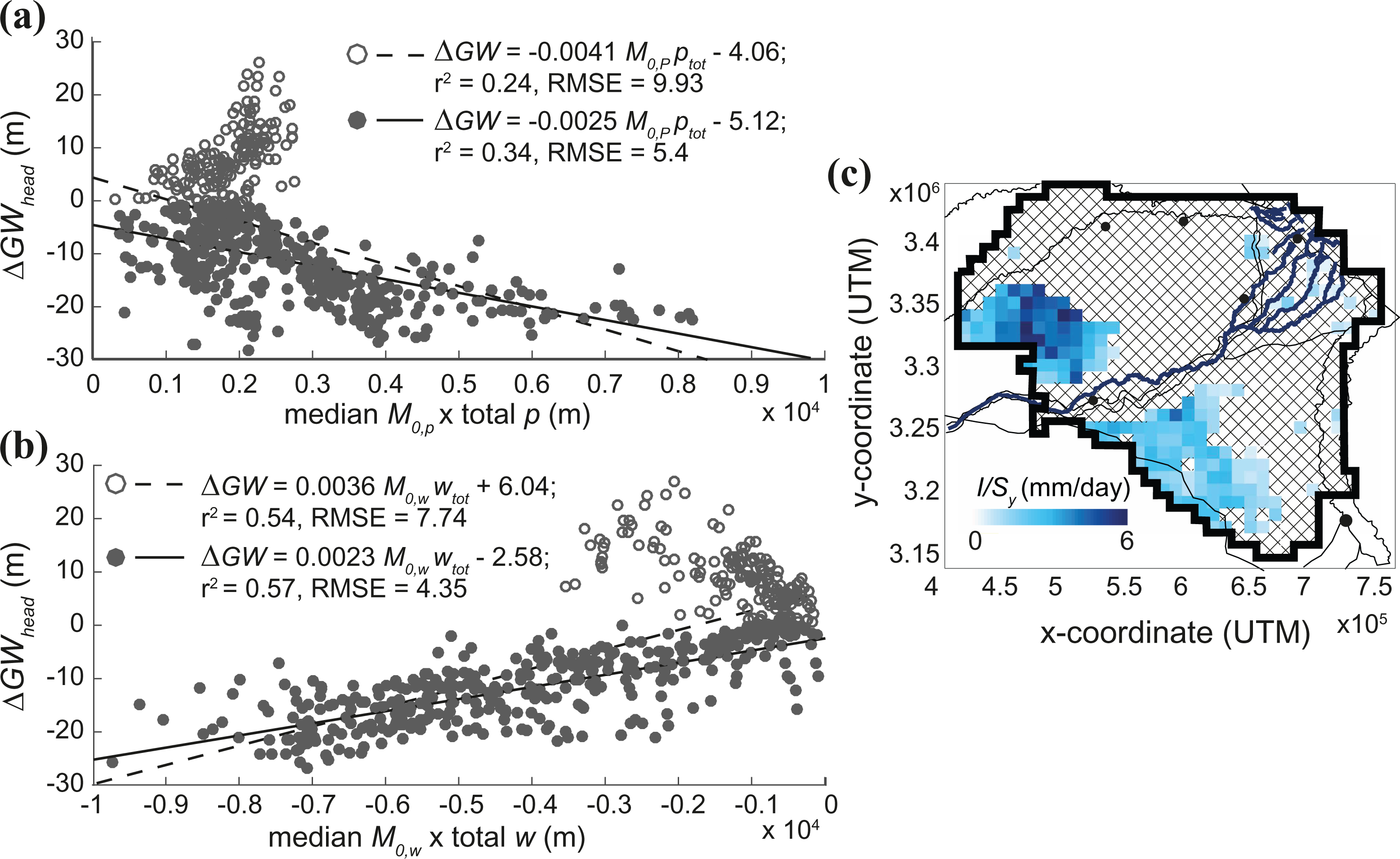
Observed groundwater level change on a cell-by-cell basis plotted against (a) the median zeroth moment for precipitation
In contrast, total abstraction (
Initially, we focused on the abstraction driver to explain the groundwater depletion observed in GRACE (Chen et al., 2014; Kumar et al., 2006; MacDonald et al., 2016; Richey et al., 2015; Rodell et al., 2009; Shah, 2009), but return flow from canal irrigation and canal leakage make up an important component for artificial recharge of the aquifer in the southwestern part of the study area. The canal network in northwestern India was constructed during the nineteenth and twentieth centuries, and leakage from canals has historically been a significant source of recharge (Cheema et al., 2014; MacDonald et al., 2016; Raza et al., 2013). The southwestern part of the region has been more dominantly irrigated by canals and tube wells, whereas the districts closer to the Himalayas were mainly irrigated by tube wells (Jeevandas et al., 2008). Groundwater level rise can be explained well by the stationary response to canal irrigation. This behavior is seen in the parts of the study area that were identified as predominantly recharged by canal irrigation by Joshi et al. (2018) on the basis of groundwater chemistry observations. The calibrated TFN model provides an estimate of modeled monthly irrigation driver scaled by the specific yield,
In general, the results show that abstraction and canal irrigation drivers can explain the first-order pattern of groundwater level change for a large part of the study area for the period 1974–2010 (Figure 3), but there are some limitations in the TFN model. As result of the limitations areas of weaker model performance can fall into two categories: locations where there were no acceptable model runs with
First, areas with more stable groundwater levels are not explained well by the combination of the four drivers. This is specifically true for the transitional area between the regions of most pronounced groundwater level rise and fall. It may also be possible that important drivers have not been adequately included within the model (Von Asmuth et al., 2008).
Second, data availability, resolution, and accuracy are all highly variable between the different drivers, and affect the outcome of the TFN model. The TFN model includes monthly values for the four drivers, but groundwater level is only available twice per year. Although this does not pose a problem for the model, the impulse response functions are continuous in time and the predictions are therefore not fixed to a certain time interval (Von Asmuth et al., 2008).
Third, observed groundwater levels in many areas continued to decline after 2006 despite the apparent stabilization of abstraction rates (Figure 4(b) and (c)). The observed groundwater level time-series shows an increasing rate of decline which may be due to limited recharge, either vertically because of water loss before reaching the water table (Hoque et al., 2007), or horizontally as surrounding aquifer bodies are depleted as well. This non-linear behavior of the groundwater level is difficult to predict with our one-dimensional implementation of the statistical TFN model approach, in which each grid cell is modeled independently, and has important implications for the sustainability of the aquifer system. Therefore, future studies that investigate the sustainability of the groundwater resource should take into account lateral groundwater flow over distances of greater than 10 km.
4 Management recommendations and wider model application
While the time series approach outlined here is highly simplified, the congruence between our key results and independent estimates of regional-scale variations in aquifer properties (Singh et al., 2017; Van Dijk et al., 2016a) and recharge mechanisms (Joshi et al. 2018) suggests that it has some predictive skill to map out the areas of maximum abstraction and their geomorphic/stratigraphic controls. This will then determine the most appropriate management strategies (Sinha and Densmore, 2016), such as where to plan artificial recharge and where to advise crop management. So what lessons can be inferred for better management strategy of this regional-scale aquifer system?
Management interventions planned by the Government of India are limited to a decrease in groundwater abstraction (via piped water supply and crop management) and an increase in recharge (via artificial recharge pits and rainwater harvesting) (CGWB, 2013). Artificial recharge schemes are likely to be most effective where the response to abstraction is rapid, but not necessarily where the stationary response
Groundwater level rise in the southwestern part of the study area is largely insensitive to temporal variations in precipitation or abstraction, and appears to be driven primarily by canal irrigation. While canal irrigation is estimated by our model rather than used as an input, the results (expressed in terms of irrigation stress normalized by specific yield) are spatially variable compared to the uniform estimates from Cheema et al. (2014). It thus appears likely that canal irrigation in this part of the basin has led to substantial aquifer recharge since 1974, which can provide insights for future management of the depleted aquifers in the study area. The sensitivity of distal areas to the canal irrigation driver also suggests that improved management of return flow, and efforts to decrease canal seepage, would help to limit water-level rises and consequent waterlogging.
It is widely recognized that there is a groundwater crisis in many of the Earth’s major aquifer systems (Richey et al. 2015; Richts et al. 2011) where unmanaged pumping of critically important groundwater resources has led to rapid rates of groundwater depletion (Famiglietti, 2014). Whilst groundwater use for irrigation has significantly increased crop yields and food security in many parts of the world (Khan and Hanjra, 2009; Siebert et al., 2010), this depletion threatens the sustainability of food production, and water and food security (Dalin et al., 2017). It is important to project changes in large-scale groundwater resources into the future to explore how best to adapt environmental policy and management (Green et al., 2011). However, most large-scale or global hydrological models, which could be used for this purpose, have a limited representation of groundwater. This has been due to the lack of groundwater level and subsurface property data, and inadequate representations of the interactions and feedbacks between human water use and management, and natural systems (Nazemi and Wheater, 2015). Addressing these issues is a current area of active research and reasonable representations of groundwater in large-scale models are beginning to appear (De Graaf et al., 2017; Pokhrel et al., 2015; Zeng et al., 2018). Parameterizing their subsurface properties, however, remains a challenge. As a first order approximation, aquifer hydraulic properties can be derived from national and global geological maps (Bhanja et al., 2016; Gleeson et al., 2014), but we consider that these will need to be refined if spatial variability in changes in groundwater levels are to be simulated adequately. Consequently, model results deviate strongly from groundwater level observations (Scanlon et al., 2018). To support the exploration of variability in aquifer properties, and investigate the response of groundwater levels to multiple-drivers, alternative parsimonious modelling approaches, such as that outlined here, will be valuable. Our study supports the conclusion of Shapoori et al. (2015c) that TFN models can provide important insights into hydrogeology, hydrological processes, and the response of the system to multiple drivers. Because they require minimal prior assumptions they are easily and rapidly transferable to other groundwater systems.
VI Conclusions
We have used a TFN time series approach to show that groundwater decline in the key regional-scale alluvial aquifer system of northwestern India over the period 1974–2010 is strongly influenced by abstraction, but that the spatial pattern of groundwater level decline is not simply based on abstraction rate alone. Time series analysis of 664 grid cells shows water levels can be predicted to first order by considering the time-varying response to four input drivers: precipitation, PET, abstraction, and canal irrigation. The results show that groundwater level decline across the northeastern part of the study area relates to the total volume of abstraction scaled by the modeled zeroth moment of the aquifer system to abstraction (
Our time series analysis provides a preliminary first-order approach for understanding the spatial controls of groundwater level changes in this critical region. The approach is effective in determining the relative importance of different stresses in driving the evolution of groundwater levels, but cannot reproduce fine-scale impacts from individual events or incorporate the complex three-dimensional stratigraphy of the alluvial aquifer system. We close by suggesting that an interdisciplinary approach that combines hydrology and geological heterogeneity should be considered in any future approaches to regional-scale aquifer management.
Supplemental material
Supplemental Material, VanDijketal_SI_SpatialVariationInGroundwaterStresses - Spatial variation of groundwater response to multiple drivers in a depleting alluvial aquifer system, northwestern India
Supplemental Material, VanDijketal_SI_SpatialVariationInGroundwaterStresses for Spatial variation of groundwater response to multiple drivers in a depleting alluvial aquifer system, northwestern India by Wout M van Dijk, Alexander L Densmore, Christopher R Jackson, Jonathan D Mackay, Suneel K Joshi, Rajiv Sinha, Shashank Shekhar and Sanjeev Gupta in Progress in Physical Geography: Earth and Environment
Footnotes
Acknowledgements
The project was initiated by W.M. van Dijk and A.L. Densmore. W.M van Dijk implemented all the data and performed the model runs and analysis together with C.R. Jackson. A.L. Densmore, J.D. Mackay, and C.R. Jackson contributed by discussing the results from the model and its implications. J.D. Mackay modeled the abstraction data. S.K. Joshi, S. Sheshank, R. Sinha and S. Gupta collected and processed the groundwater level data. The authors would like to thank Antoine Lafare and Edwin Sutanudjaja for earlier discussions. Constructive and positive reviews by two anonymous reviewers helped to clarify and strengthen the manuscript. The time-series analysis model AquiMod is free available online through the British Geological Survey (https://www.bgs.ac.uk/research/environmentalModelling/aquimod.html). The meteorological data of the Indian Meteorological Department is publicly available from a web portal (![]() ). To obtain the input data and model used in this paper, please contact the corresponding author.
). To obtain the input data and model used in this paper, please contact the corresponding author.
Declaration of conflicting interests
The author(s) declared no potential conflicts of interest with respect to the research, authorship, and/or publication of this article.
Funding
The author(s) disclosed receipt of the following financial support for the research, authorship, and/or publication of this article: This project is supported by the UK Natural Environment Research Council and the Indian Ministry of Earth Sciences under the Changing Water Cycle - South Asia program (Grant NE/I022434/1). The abstraction modeling was supported by the UK Natural Environment Research Council (Grant NE/I022590/1).
Supplemental material
Supplemental material for this article is available online.
References
Supplementary Material
Please find the following supplemental material available below.
For Open Access articles published under a Creative Commons License, all supplemental material carries the same license as the article it is associated with.
For non-Open Access articles published, all supplemental material carries a non-exclusive license, and permission requests for re-use of supplemental material or any part of supplemental material shall be sent directly to the copyright owner as specified in the copyright notice associated with the article.