Sage Journals: Discover world-class research

Abstract

This paper constructs a regional dynamic macroeconomic model with an eclectic, broadly Keynesian and behavioural flavour. The model, which is parameterized on Scottish data, is used to identify the impact of expectations and business confidence on regional resilience. Simulations compare the evolution of the regional economy after a temporary negative export shock under a range of investment functions. The mainstream perfect foresight formulation generates a reduction in activity, which is small and is limited to the duration of the shock. The heuristic-based, imperfect-information investment models produce more negative, longer-lasting and unstable adjustment paths.

Keywords

Regional resilience computable general equilibrium modelling behavioural economics Keynesian economics

Introduction

Economists have faced strong and widespread criticism because of their inability to predict the onset of the financial crisis, question the institutions that created that crisis and, more especially, provide subsequent appropriate policy advice (Earle et al., 2017; Kwak, 2017; Wren-Lewis, 2015). A key aspect of this critique is the perceived malign influence of abstract theory and, in particular, general equilibrium analysis. However, there is an obvious attraction to adopting a method that models the economy as a whole, simultaneously incorporating both micro- and macroeconomic perspectives in an internally consistent and flexible manner. Moreover, it is a misconception that general equilibrium analysis is constrained by the conventional neoclassical straightjacket.

In the early development of computable general equilibrium (CGE) analysis, an important strand concerned the modelling of developing economies (Taylor, 2011). These models typically exhibited clear non-neoclassical properties, in terms of behaviour and institutions. However, increasingly CGE analysis has been dominated by models taking a more purely neoclassical position. This is unfortunate for two reasons: first, rigidity is imposed on a form of modelling, one of whose strengths is flexibility; and second, strict rationality often drives the adoption of an extreme set of assumptions in such models.

The present paper has three primary aims. The first is to show that CGE modelling is an extremely flexible tool that can be used to illustrate and explore a wide range of approaches to regional analysis. The second is to construct a regional economic model that incorporates behavioural/Keynesian insights, motivated by the work of Joan Robinson and Daniel Kahneman (Harcourt, 1995; Lewis, 2017). The third is to use this model to investigate the role that firm agency and decision-making play in determining regional resilience (Martin, 2012; Martin and Sunley, 2015). We use the CGE framework as a test-bed to study the impact of varying a key determinant of dynamic resilience in a controlled theoretical and empirical setting (Wei et al., 2018).

Background

The basic characteristics of the neoclassical research programme are summarized by Becker (1976: 5): ‘The combined assumptions of maximizing behaviour, market equilibrium, and stable preferences, used relentlessly and unflinchingly, form the heart of the economic approach as I see it.’ Both Arrow and Debreu received the Nobel Prize in Economics, at least in part for their separate work on the existence of general equilibria under these neoclassical assumptions, even though this analysis has almost no practical application. However, important welfare results apply under such equilibria; for example, Rodrik (2016) claims that the First Theorem of Welfare Economics – essentially that universal perfect competition in an economy in general equilibrium ensures a Pareto optimal outcome – is one of the crown jewels of economics. In this way, standard neoclassical theory is an interweaving of normative and positive elements, purporting not only to account for how the economy actually operates but also how it ought to operate, if desirable consumer welfare ends are to be achieved (Weimann et al., 2015).

But while the neoclassical research programme is presented as being theoretically progressive, its empirical success is much less certain. In the ‘Anomalies’ section of the Journal of Economic Perspectives, Thaler teased other economists with instances of their own behaviour that seemed irrational and therefore inconsistent with standard microeconomic theory (Thaler, 2015). Similarly, game theory extensively studied rational strategic behaviour under perfect and imperfect information, but classroom experiments with many simple games failed to replicate the outcomes predicted by theory. Moreover, the imposition of the efficient markets hypothesis and rational expectations led to the hegemony in the academic macroeconomic modelling literature that failed to foresee the financial crash. But much more importantly, these macroeconomic models also proved of little use in dealing with the subsequent aftermath (Wren-Lewis, 2015, 2018).

Initially, CGE modelling included an eclectic, non-neoclassical primarily development stream (Taylor, 2011), and more pragmatic CGE modelling frameworks still exist. However, these approaches have increasingly been swamped by off-the-shelf conventional CGE models, wholly populated with rationally maximizing agents and a consistently neoclassical base. These models assume perfectly competitive markets for goods and factors, and well-behaved production and consumption functions, where dynamic, perfect foresight is typically imposed and balanced budget fiscal rules applied. A central notion is that all decisions are rational and not subject to systematic error. It is important to stress that such models are not just theoretical tools but are actually used to inform policy debate (HM Treasury and HM Revenue and Customs, 2014). They reflect the fact that economics is typically presented as comprising a single dominant model, fundamentally based on universal and consistent rational behaviour.

As a matter of principle, Joan Robinson fought against such a uniform approach, recognizing that appropriate economic analysis should reflect the social and administrative conditions under which it is applied. Further, changing key assumptions is a useful form of thought experiment (Robinson, 1960; Rodrik, 2016). She was particularly interested in alternative conceptions of the economy and how these varied across different schools of economic thought, often carrying a clear ideological charge (Robinson, 1962). As Amos Tversky, co-author of Nobel-cited work with Kahneman, states: ‘Reality is a cloud of possibilities, not a point’ (Lewis, 2017: 312). In analysing a capitalist economy, Joan Robinson was influenced strongly by Keynes and especially emphasized the role of animal spirits and liquidity preference in determining investment and therefore breaking the direct link with savings.

In this respect, is it reasonable to assume that economic agents are rational and fully informed? Kahneman (2012) makes the distinction between Type 1 and Type 2 thinking. Type 1 thought processes cover automatic responses to stimuli, associative thinking and heuristics (or rules of thumb). It is ‘low-cost’ mental activity. Humans find it easy to do and adopt Type 1 thinking as a default. Type 2 mental activity involves simultaneously considering or comparing previously stored information. These are ‘high-cost’ thought processes that humans typically avoid through the use of mental short-cuts, gut feelings or intuition. So, while neoclassical general equilibrium theory implies that all decisions are made using Type 2 processes, there is extensive evidence that much behaviour by economic agents is driven by Type 1 thinking. As discussed more fully later in the paper, choices involving numerous outcomes, particularly those incorporating intertemporal optimizing and uncertainty, are typically not taken fully rationally. Moreover, our decisions are very easily influenced by the conditions under which the decision is taken, including framing.

When justifying the use of what appear to be unrealistic assumptions about agents’ knowledge, computational powers and rationality, economists typically find the arguments given by Friedman (1953) convenient and sufficient. The core claim is that the key test of the validity of a theory is whether it correctly predicts, and for prediction it is irrelevant whether the assumptions of the theory are correct. In this case, it does not matter whether agents consciously maximize, as long as they act ‘as if’ they maximize. As Hausman (1992: 162) claims: ‘Friedman’s essay, “The Methodology of Positive Economics” … is the only essay on methodology that a large number, perhaps a majority, of economists have ever read.’

However, a number of points need to be made concerning the defence Friedman mounts. The first is that almost all those writing specifically on the methodology of economics have been critical of Friedman’s position (Hausman, 1992: 163). Second, economists typically adopt a particular variant of this approach. This is that while individuals might deviate from rational maximizing behaviour, such deviations are in some sense random and not systematic in nature. However, the strength of the behavioural critique is that many errors made using Type 1 thinking are systematic. Particularly well-known examples are loss aversion and inconsistent time preference. Third, as we argue above, a primary difficulty for conventional economics has been precisely its inability to accurately predict both macro and microeconomic behaviour. Finally, even if neoclassical ‘as if’ theories did give accurate predictions, these would not be adequate explanations (McLachlan and Swales, 1990). This seems particularly problematic where welfare implications are attributed to economic outcomes.

It is often argued that there has been a behavioural revolution in economics. However, such a revolution seems to be only skin deep; behavioural economics essentially appears to have been accommodated within the conventional neoclassical framework. As Angner (2012: xv) states, ‘while behavioural economists reject the standard theory as a descriptive theory, they typically accept it as normative theory’. Further, ‘much of behavioural economics is a modification or extension of neo-classical theory’. Therefore, while a behaviouralist approach would seem to imply a rather radical questioning of the standard economic theory, its actual impact has been much more muted. In this paper we wish to explore how behavioural concepts could be more firmly anchored in a flexible general equilibrium modelling framework. Very specifically, we wish to show how taking alternative behavioural/Keynesian approaches to investment behaviour affects the modelling of regional resilience.

Regional resilience

Regional resilience can be broadly described as the ability of a system to recover from or to adapt to external (adverse) shocks, with the literature identifying three main forms: engineering, ecological and evolutionary (this taxonomy is discussed in detail, for example, by Davoudi (2012) and Martin and Sunley (2015)). Engineering resilience is a measure of the system’s capacity to return to equilibrium after a disturbance (Holling, 1973, 1996). Ecological resilience focuses on a system’s ability to absorb external shocks before it is changed in structure (Holling, 1996; Walker et al., 2006). This differs from engineering resilience in that it acknowledges the possibility of multiple equilibria following a shock. Finally, evolutionary resilience challenges the idea of equilibrium and considers the ability of a system to transform endogenously as it adapts to disturbances (Simmie and Martin, 2010). Both ecological and evolutionary resilience imply the possibility of hysteresis and path dependence.

The region’s resilience can be expressed in terms of four separate elements (Martin et al., 2016). These are the region’s vulnerability and resistance to the shock and its subsequent adaptability and recoverability. Martin and Sunley (2015: 3) maintain that while resilience is a prominent and potent concept in regional analysis, ‘there is as yet no theory of regional economic resilience’. They identify a large number of factors that potentially affect resilience, with a key group, labelled ‘agency and decision making’, comprising perception, expectations, confidence and convention. However, they maintain that we ‘know surprisingly little about the role of market psychology and decision-making in shaping agents’ behaviour following a major economic disruption, nor about how such behaviour and decision-making interact with local context. Yet, arguably, expectations, confidence and attitudes may prove to be critical factors’ (Martin and Sunley, 2015: 35).

There is a small CGE literature that complements case studies and econometric work in the analysis of regional resilience. Di Pietro et al. (2020) use the RHOMOLO CGE model to identify the differential resilience of individual NUTS 2 (European Nomenclature of Territorial Units for Statistics at level two) regions to EU-wide temporary demand and supply shocks, focusing on the role of industrial and trade structure. On a smaller scale, Rose (2004) discusses CGE as ‘a state of art tool’ for the analysis of the behaviour of individual regions in response to adverse, focused supply-side shocks, such as natural disasters. He also emphasizes the behavioural nature of resilience and highlights that decisions related to resilient actions may violate established economic norms such as rational behaviour on which these models are often grounded (Rose, 2004, 2006; Rose and Liao, 2005).

In the present paper, the CGE framework is employed as a test-bed in order to study the effect of altering a key determinant of engineering resilience in a controlled theoretical and empirical environment. Specifically, the model identifies how variations in investment behaviour, driven by differences in confidence and expectations, affect the size of the impact, the rate of descent and the subsequent speed of recovery associated with a temporary negative demand shock. This is done while holding constant the size and nature of the initial shock, together with other key elements of the regional economy, including other determinants of resilience such as the degree of wage and price flexibility.

A behavioural regional CGE model

In this paper we demonstrate the potential flexibility of CGE modelling and take the first step in developing a variant, using the AMOS modelling framework for Scotland, which incorporates behavioural assumptions in a fundamental way.¹ The primary focus is to provide alternative specifications of the investment function, some of which incorporate behavioural characteristics. However, we also discuss behavioural interpretations of other elements of the model, such as household consumption and the labour market.

A key characteristic of CGE models is their potential flexibility. In the present case we retain a standard supply side through imposing a competitive market structure in which firms are assumed to maximize profit. Essentially this means that in the long run production occurs at minimum cost with a constant profit rate across all sectors. This is a condition imposed by Keynesian, Marxian, neo-Ricardian and standard neoclassical models. Also, it does not seem an unrealistic assumption, given that in many sectors computerization, together with improved communications and connectivity, have allowed more effective cost minimization. The behavioural elements are introduced in the consumption, labour market and investment decisions.

Behavioural research points to a degree of irrationality in individual decision-making. Some inconsistent behaviour is systematic, such as loss aversion, distorted time preference and difficulty in dealing with uncertainty and probability. Other inconsistencies are more idiosyncratic, so that, for example, an individual’s response to specific choices might depend crucially on how these choices are framed. Further, firms are aware of such consumer informational asymmetries and irrationality and use these in their own interests through targeted advertising, political lobbying and other types of promotion.

In the present model we take consumption to be consistent with standard theory. However, we do not consider these choices necessarily optimal in any normative sense. Therefore, while we model household expenditure using deterministic consumption functions that are price- and income-sensitive, we do not assume that these represent welfare maximization under constraints. Nor do we have a measure of welfare that can be used to compare alternative equilibria. Consumption expenditure is simply a constraint on the firm’s profit-maximizing behaviour. There are numerous examples of firms and industries acting against their own customers’ interests, typically through the manipulation of asymmetric information or the encouragement of addictive behaviour (Eyal and Hoover, 2014; Harford, 2017; Keefe, 2017).

In the standard CGE neoclassical approach to the labour market, the worker simply trades off leisure for wage income. The wage and other employment conditions are not determined by negotiation between the firm and the worker (or their representative). Unemployment is treated as voluntary leisure. Behavioural economists have taken a different view, stressing mechanisms such as nominal wage stickiness and the importance of the worker’s reference point in determining the wage bargain (Kahneman, 2012: 290; Thaler, 2015: 131–132). Similarly, empirical work identifies unemployment as being a particularly potent and persistent cause of self-reported reductions in well-being (Weimann et al., 2015). Clearly there is a strong argument for considering the labour market, from both a practical and policy perspective, in a bargaining or imperfectly competitive manner.

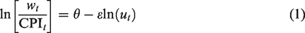
Variants of the AMOS CGE model offer alternative labour market options, including closures exhibiting nominal and real wage rigidity. In the simulations reported in this paper we choose not to treat wage determination in the conventional neoclassical manner, but rather as governed by social and legal institutional constraints. Specifically, we characterize the labour market as operating through a wage curve, where the real wage is a function of the unemployment rate.²

There is extensive evidence for such a labour market specification, which can be motivated through a bargaining or efficiency wage interpretation (Blanchflower and Oswald, 2005). In either case there is involuntary unemployment so that workers cannot freely choose whether to work or not, so that there would be unemployed workers prepared to work at the existing real wage. The wage curve takes the form:

\ln [\frac{w_{t}}{{CPI}_{t}}] = θ - ε \ln (u_{t})

(1)

where w represents the nominal take-home wage, CPI is the consumer price index, u is the unemployment rate and subscript t stands for the time period. The parameter

ε

is the elasticity of the real wage with respect to the unemployment rate, and takes a value of 0.1;

θ

is calibrated so as to reproduce the base-year data (Galvez, 2014; Layard et al., 2005). It should be stressed that this approach is not novel in itself; an extensive discussion of labour market closures in CGE models is given by Boeters and Savard (2011). However, we believe that using a wage curve is consistent with a behavioural orientation.

In a conventional CGE model, the firm plays a totally passive role. The representative household is characterized as both the supplier of productive inputs and the consumer of commodities. Technology transforms inputs into outputs; there are markets, but no other intervening institutions. This has the implication that both saving and investing are undertaken by the household, becoming essentially the same activity driven by the need to optimize consumption over time. This runs counter to a key element of Keynesian analysis, which is that savings and investment are actions taken by two quite separate groups of people.

Moreover, behavioural approaches have strongly questioned the notion that savings are determined in a rational, optimal manner, as a trade-off between present and future consumption (Akerlof and Shiller, 2009). In the present model we adopt a Keynesian saving function in which savings are a fixed share of disposable income, with the interest rate determined in extra-regional (national and international) financial markets. Saving and investment are therefore not equilibrated through movements in the interest rate, which is governed by liquidity preference. They therefore have to be analysed separately.

The CGE model used here exhibits regional characteristics, in that we impose no balance of payments or public sector budget constraint (Lecca et al., 2013). In the present simulations we hold government expenditure constant in real terms and tax rates fixed. This primarily reflects the system of devolved public finances operating in the UK in the time period for which the model is calibrated. The Scottish government had essentially no control over tax rates or total public expenditure in Scotland, which was set by the UK government, independent of the taxes raised in Scotland.³

Alternative investment behaviour

In this paper, a particular focus is the effect that different expectation-formation processes have on the level of investment. A central aim is to use this model to demonstrate the role that firm agency and decision-making play in determining the response of overall regional economic activity to a temporary exogenous demand disturbance. Essentially, we use the CGE framework as a test-bed to study the impact of varying a key determinant of regional engineering resilience (Martin, 2012; Martin and Sunley, 2015; Wei et al., 2018).

Investment necessarily commits the firm to costs in advance of future revenues. In making an investment decision, the firm has to predict the time path of relevant exogenous disturbances and the endogenous reaction of the rest of the economic system to these shocks. The part played by expectations is clearly important, with Keynes stressing the role of uncertainty, framed in terms of animal spirits and liquidity preference. This aspect of his work is emphasized by Robinson (1962), and these ideas are strongly supported by behavioural economists such as Akerlof and Shiller (2009). Certainly in terms of financial investment, as Thaler (2015: 209) states: ‘Keynes … was a true forerunner of behavioural finance.’ Although authors have previously explicitly linked Keynesian and behavioural approaches, the discussion of animal spirits in behavioural economics is extremely limited (Pech and Milan, 2009). That is to say, there seems a dearth of literature as to how individuals predict the future, and how this affects investment decisions.⁴

The core neoclassical model is characterized by perfect foresight and, in a stochastic context, rational expectations. All economic actors are assumed to correctly foresee the future and act optimally, given that all others are similarly optimizing using a correct (neoclassical) model of how the economy operates. While this is supposedly a market economy, many futures markets do not exist so that individuals have to be able to correctly forecast the response of markets in the future to prior exogenous shocks. Essentially, mainstream economists are routinely working on models that assume that economic actors can already solve such models. Behavioural and Keynesian economists disagree with this approach and argue that individuals simply do not operate in this way.

There are many experimental studies of choices under risk, where the odds of particular outcomes occurring are known (Kahneman, 2012). Investigating risk in such a restricted and controlled setting sharpens the behavioural results and makes their existence absolutely clear. This work shows that such choices are often inconsistent, failing the very lowest form of rationality, which is clearly problematic for conventional economic theory.

However, the actual decisions that economic agents have to make are typically much more complex. First, they involve consistent, exponential discounting of future costs and benefits. But there is clear evidence of the extensive use of hyperbolic discounting that generates time-inconsistency and self-control problems (Laibson, 1996; Loewenstein and Prelec, 1992). Second, in the perfect foresight model individuals need to be able to predict and optimally act upon the behaviour of others. But evidence from experiments with the centipede game suggests that in practice individuals find this difficult to do, even in a relatively straightforward situation (Angner, 2012). Where individuals have differing levels of skill, experience or information, the optimal decision for any one player depends not on the actual optimum but what they think others believe to be the optimum (Cartwright, 2011: ch.6; Keynes, 1936). Further, with investment, even if agents could calculate what the optimal future capital levels should be for individual sectors, for example, there would still be an issue in practice about coordinating the actual investment decisions by individual firms. In this situation there seems no obvious focal point.

In the simulations whose results are reported in the section ‘Simulation results’, we introduce an exogenous unanticipated temporary (five-period) 5% contraction in the demand for all exports. We use three alternative investment functions to determine the subsequent evolution of industrial capital stocks: perfect foresight; myopic expectations; and imperfect foresight. Each of these investment models exhibits partial adjustment in the sense that there are adjustment costs in a similar manner as Malakellis (1997) and Dixon et al. (2005). Each is motivated by a different expectations-formation process.

Perfect foresight

In this case, although the disturbance is unanticipated, its subsequent size and duration is known, as are the subsequent market reactions. Within the AMOS model, this represents the standard, state-of-the-art neoclassical approach. In this case, in each sector the path of private investment is obtained by maximizing the present value of the representative firm’s cash flow:

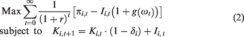
\begin{matrix} Max \sum_{t = 0}^{\infty} \frac{1}{{(1 + r)}^{t}} [π_{i, t} - I_{i, t} (1 + g (ω_{t}))] \\ subject to K_{i,}_{t + 1} = K_{i, t} \cdot (1 - δ_{i}) + I_{i, t} \end{matrix}

(2)

The cash flow is given by profit, $π_{i, t}$ , less private investment expenditure, I_i,t, subject to the presence of adjustment cost $g (ω_{i, t})$ where $ω_{i, t} = \frac{I_{i, t}}{K_{i, t}}$ and δ is the rate of physical depreciation.

Myopic expectations

In the myopic expectations model, firms take the expected future output attempt to be the present output. They therefore adjust their capital stock to the desired level determined by present input prices and output, although, because of adjustment costs, this process is not instantaneous. This implies that in these models, gross investment in time period t is equal to depreciation plus some proportion, v, of the difference between the desired capital stock in the next time period, $K_{i, t + 1}^{*}$ , and the actual present capital stock, $K_{i . t}$ . This implies:

I_{i, t} = v [K_{i, t + 1}^{*} - K_{i . t}] + δ K_{i, t}

(3)

The desired capital stock in period t + 1 is determined by the output price and cost of capital in time period t, and the expected output in period t + 1, $Q_{i, t + 1}^{e}$ , so that:

K_{i, t + 1}^{*} = K_{i} (Q_{i, t + 1}^{e}, p_{i, t}, r_{i, t})

(4)

The firm takes the existing industry output as the best estimate of output in the next period, so that in the myopic case:

Q_{i, t + 1}^{e} = Q_{i, t}

(5)

Equations (3)–(5) then make up the investment function with myopic expectations, a formulation that has been used previously in AMOS and other CGE simulations (Dixon and Jorgenson, 2013; Lecca et al., 2013).

Imperfect foresight

In the imperfect foresight model, firms are forward-looking but instead of basing their expectations on fully solving the general equilibrium model of the economy, they use a simple heuristic. This heuristic is that an industry’s future output will be a linear extension of the past output trend.

Rosling (2018) notes the strong tendency to project present trends into the future along a linear track. He argues that being able to predict linear paths of projectiles would confer a survival advantage to human beings in the early stage of their evolution and that this remains a prominent part of our mental toolkit. A similar phenomenon, in a micro-setting, is the mistaken ‘hot hand’ belief among basketball players (Gilovich et al., 1985). This is the conviction that a player whose shooting accuracy has been particularly good in the immediate past will continue to exhibit this accuracy in the immediate future. In the context of regional resilience, note also the linear employment trajectories used by Martin and Sunley (2015: figures 2 and 3).

As far as we are aware, this is the first use of such an imperfect foresight heuristic in a CGE model. It is operationalized by again adopting equations (3) and (4), but by determining the expected output at time t + 1 as a linear projection of past output change over the last n periods, so that:

Q_{i, t + 1}^{e} = Q_{i, t} + \frac{Q_{i, t} - Q_{i, t - n}}{n} = \frac{(n + 1) Q_{i, t} - Q_{i, t - n}}{n}

(6)

Model calibration, parameterization and simulation strategy

The CGE model is parameterized on a social accounting matrix for Scotland constructed with data for 2010.⁵ There are 30 industrial sectors. The real wage is determined by the operation of the wage curve together with a fixed labour force.⁶ In all sectors the Armington trade elasticities are set to a value of 2 (Gibson, 1990) and the elasticities of substitution in production between labour and capital and between value-added and intermediates are 0.3 (Harrassova, 2018; Harris, 1989).

We simulate the impact of the temporary exogenous demand shock in the following way. The model is initially calibrated to be in long-run equilibrium. This means that if the model were run in period-by-period mode with no change in exogenous variables, the value of none of the endogenous variables would change. In period 1 we introduce a 5% step reduction in the demand for all Scottish exports, which is maintained for a further four periods and then reversed. This means that in period 6 the export demand function returns to its original level.⁷ The model is then run forward for a further 40 periods. Each period is equal to one year, which is consistent with the annual data used for parameterization.

We chose this particular demand disturbance solely for pedagogic reasons. Regional economies are typically very open to trade and adverse demand shocks are likely to come from that source. We shock all exports so that the results are more representative, not being distorted by the characteristics of a specific industry. The five-period length of shock allows us to investigate in more detail the dynamic relationship between output decline and investment under different expectation-formation regimes in the contraction phase. The impact of varying the length of the shock is investigated elsewhere.⁸

In the long run, which is the time interval over which capital stocks are fully adjusted, the economy moves to a new steady-state equilibrium. Because the model generates no hysteresis effects and the disturbance is transitory, in the reported simulations variables ultimately return to their original values, so that we are modelling engineering resilience in this instance.⁹ However, while the model is parameterized on a static equilibrium, the results can also be interpreted as fluctuations around a constant growth trajectory. We simulate with three versions of the model with the different expectation-formation characteristics informing the investment decision, as outlined in the previous section. In all the models the results for all the endogenous variables are reported as percentage changes from the corresponding base-year values.

Simulation results

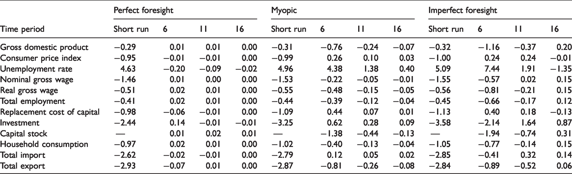
Table 1 reports the values that a set of key endogenous economic variables take for periods 1, 6, 11 and 16. Period 1 corresponds to the short run, where the negative demand shock has been introduced but the capital stocks are still fixed. Subsequently, in each industry, investment updates the capital stock between periods. Period 5 is the last period in which the negative demand shock operates, so that from period 6 the initial export demand parameter is reinstated. Detailed period-by-period impacts on investment and GDP are given in Figures 1 and 2.¹⁰ Note that by around period 40 all models have returned to long-run equilibrium, but that their adjustment paths are very different. We begin by discussing the simulation results where investment is determined through perfect foresight.

Table 1.

Impact of a temporary 5% reduction in exports on key macroeconomic variables (% change from baseline values).

	Perfect foresight				Myopic				Imperfect foresight
Time period	Short run	6	11	16	Short run	6	11	16	Short run	6	11	16
Gross domestic product	−0.29	0.01	0.01	0.00	−0.31	−0.76	−0.24	−0.07	−0.32	−1.16	−0.37	0.20
Consumer price index	−0.95	−0.01	−0.01	0.00	−0.99	0.26	0.10	0.03	−1.00	0.24	0.24	−0.01
Unemployment rate	4.63	−0.20	−0.09	−0.02	4.96	4.38	1.38	0.40	5.09	7.44	1.91	−1.35
Nominal gross wage	−1.46	0.01	0.00	0.00	−1.53	−0.22	−0.05	−0.01	−1.55	−0.57	0.02	0.15
Real gross wage	−0.51	0.02	0.01	0.00	−0.55	−0.48	−0.15	−0.05	−0.56	−0.81	−0.21	0.15
Total employment	−0.41	0.02	0.01	0.00	−0.44	−0.39	−0.12	−0.04	−0.45	−0.66	−0.17	0.12
Replacement cost of capital	−0.98	−0.06	−0.01	0.00	−1.09	0.44	0.07	0.01	−1.13	0.40	0.18	−0.13
Investment	−2.44	0.14	−0.01	−0.01	−3.25	0.62	0.28	0.09	−3.58	−2.14	1.64	0.87
Capital stock	—	0.01	0.02	0.01	—	−1.38	−0.44	−0.13	—	−1.94	−0.74	0.31
Household consumption	−0.97	0.02	0.01	0.00	−1.02	−0.40	−0.13	−0.04	−1.05	−0.77	−0.14	0.15
Total import	−2.62	−0.02	−0.01	0.00	−2.79	0.12	0.05	0.02	−2.85	−0.41	0.32	0.14
Total export	−2.93	−0.07	0.01	0.00	−2.87	−0.81	−0.26	−0.08	−2.84	−0.89	−0.52	0.06

Figure 1.

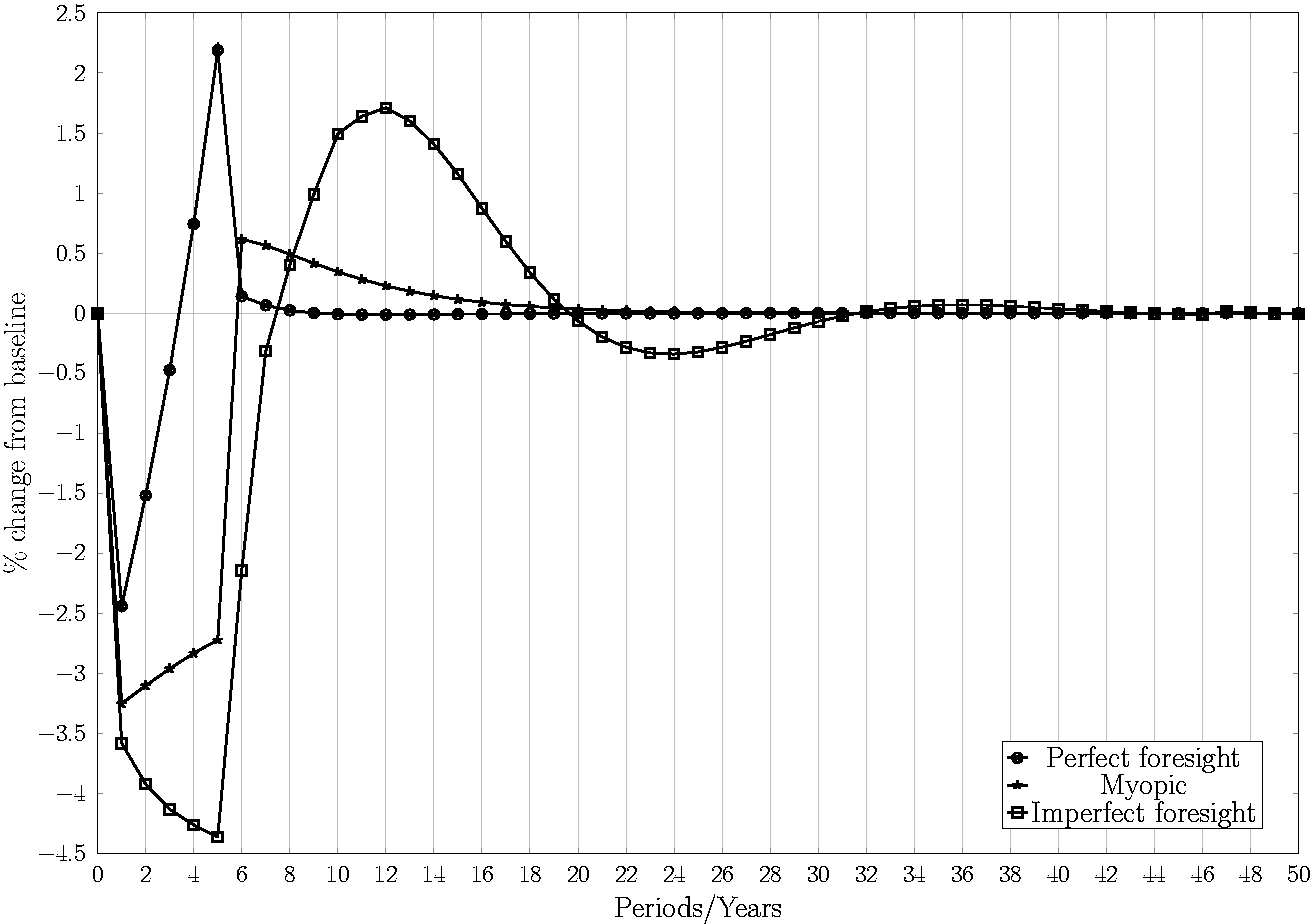
Period-by-period adjustment of investment.

Figure 2.

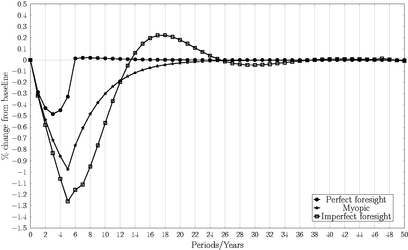
Period-by-period adjustment of GDP.

Perfect foresight

For the perfect foresight model, the period-1 (short-run) response to the 5% negative export demand shock is a fall in aggregate economic activity. GDP, employment, investment and exports decrease by 0.29%, 0.41%, 2.44% and 2.93% respectively, accompanied by a 4.63% increase in the rate of unemployment with a 0.51% decline in the real wage. The downward movement in production also reduces capital rentals and this, together with the fall in the wage, is reflected in the 0.95% decline in the CPI. The decrease in factor incomes and employment reduces household consumption by 0.97%.

Note first that the period-1 reduction in domestic prices increases Scottish competitiveness so that the fall in total exports is less than the 5% exogenous reduction in export demand. Second, there is a relatively large short-run fall in investment. In the initial equilibrium, investment just covers depreciation. The reduction in investment occurs as firms attempt to downwardly adjust their capital stock, producing an accelerator effect where the proportionate fall in investment is greater than the corresponding reduction in output.

Figure 1 indicates that in the perfect foresight case, investment is at its minimum point in period 1. From periods 2 to 5, investment is increasing, and in both periods 4 and 5 is actually above the base-year value. This anticipates the return of the initial export demand conditions and takes advantage of low capital replacement costs. Its maximum (period 5) value is 2.19%, and in period 6 the aggregate capital stock is also slightly higher than its initial value.

In tracking aggregate economic activity, note that the reduction in demand associated with lower investment expenditure is less in the periods immediately after period 1. However, the negative impact on supply from lower capacity is initially more powerful. As Figure 2 indicates, this leads to falling GDP and employment in periods 2 and 3, reaching minimum values of 0.48% and 0.47% below base, respectively.

In the first period in which the exogenous export demand shock is reversed, GDP, employment and aggregate capital stock are higher than in the base period. However, there is still less than full sectoral adjustment to the restored export demand, with exports 0.07% below their initial value. In subsequent periods investment falls and asymptotically approaches the base-year level from above. GDP is maximized at a positive value of 0.02% in period 8. By period 11 the economy is very close to its initial equilibrium.

Myopic expectations

Variation in the short-run (period 1) results across simulations is driven solely by differences in the scale of the negative demand shocks coming through reduced investment. In the myopic expectations case, firms attempt to adjust their capital stock, taking present output as the best estimate of future output. This is associated with a 3.25% fall in investment in period 1, which is greater than the reduction under perfect foresight, producing a fall in GDP, employment, household consumption and exports of 0.31%, 0.44%, 1.02% and 2.87%, respectively.

As in all the period-1 results, the relative size of the GDP and employment impacts is explained by labour market flexibility. Employment falls by a greater proportionate amount than GDP because in the short run capital stock is fixed and cannot immediately be fully adjusted downwards. The proportionate reduction in household consumption is then greater than that in employment because household income is affected by both the fall in employment and the accompanying decline in the real wage.

In the myopic case, in periods 2–5 – that is, in the remaining period during which the negative export shock operates – investment rises slightly but remains well below the initial level. GDP falls continuously while the export shock is in place and by period 5 is at its minimum, 0.97% below its base-year value. In period 6 investment rises to 0.62% above its initial value, but GDP and employment are still 0.76% and 0.39%, respectively, below their initial values. The low level of aggregate economic activity in period 6 reflects the reduced capital stock, which is 1.38% below its base-year figure. This means that even though employment, and therefore also the real wage, is below its initial level, domestic prices are not. Again the negative effect on competitiveness reduces aggregate economic activity.

From period 6, investment approaches its initial value asymptotically from above, while GDP, employment and household consumption asymptotically approach theirs from below. However, it takes an extended length of time before the economy is back in long-run equilibrium. For example, in periods 11 and 16 GDP is still 0.24% and 0.07% respectively below its base-year level.

Imperfect foresight

In the myopic case, firms make investment decisions using the heuristic that present output is the best estimate of future output. However, as we have seen, output varies systematically after the introduction of the export demand shock. In particular, both the adverse demand and supply effects of reduced investment and the resultant fall in the capital stock exacerbate the initial impact of the drop in export demand. This means that in periods 1–4 the myopic firms will always overestimate, and then in subsequent periods underestimate, the next-period output. While it appears unrealistic that firms have a correct model of the economy, it also seems equally unlikely that they would not update the investment heuristic. In this case we assume that the firm estimates the output in the next period as a linear projection of the evolution of output, as given in equation (6), over the past four periods.

This variant of the model produces the largest period-1 fall in investment at 3.58%. Further, during the subsequent interval up to, and including, period 5, investment is continuously falling. Investment, GDP, employment and household consumption all reach their minima in period 5 at 4.36%, 1.26%, 0.98% and 1.61%, respectively, down on their initial levels.

When the export shock is reversed, investment increases but only surpasses the base-year value in period 8. It reaches a maximum of 1.71% above base in period 12 but drops below base again in period 19. There is clear overshooting that causes similar, but lagged, damped cycles in GDP, employment and household consumption. Employment and household consumption exceed their initial values in period 12 and GDP in period 13. These variables all reach a maximum at period 16 and fall below their initial values in period 25.

Comparing the three scenarios: Implications for regional resilience

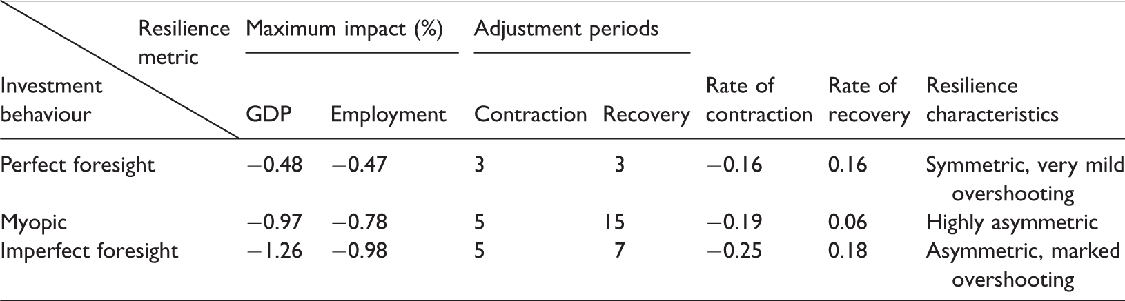
In Table 2 we compare the pattern of resilience revealed by the AMOS model when alternative investment functions are employed, reflecting differences in the assumed knowledge and confidence exhibited by business organizations when making investment decisions. The table compares the simulation results from the three cases outlined in the previous section using the following metrics: the maximum reductions in GDP and employment; the length of the time periods over which the economy contracts and recovers; and the rates of contraction and recovery. The time period for the contraction is calculated to the period in which the size of the GDP reduction is at its maximum value. The recovery is calculated as the number of periods from the maximum reduction to the first period in which GDP equals the original level.¹¹ Table 2 also comments on the symmetry and any overshooting exhibited in the three adjustment paths.

Table 2.

The resilience of the Scottish economy to a temporary (five-period) 5% reduction in export demand.

ResiliencemetricInvestmentbehaviour	Maximum impact (%)		Adjustment periods		Rate of contraction	Rate of recovery	Resilience characteristics
ResiliencemetricInvestmentbehaviour	GDP	Employment	Contraction	Recovery	Rate of contraction	Rate of recovery	Resilience characteristics
Perfect foresight	−0.48	−0.47	3	3	−0.16	0.16	Symmetric, very mild overshooting
Myopic	−0.97	−0.78	5	15	−0.19	0.06	Highly asymmetric
Imperfect foresight	−1.26	−0.98	5	7	−0.25	0.18	Asymmetric, marked overshooting

It is important to stress that we are here solely considering engineering resilience; that is, the reaction of the economy to a temporary negative shock that does not affect the economy’s long-run trajectory. The ‘plucking’ model is often cited as an appropriate approach to this type of resilience (Friedman, 1993). However, we wish to emphasize strongly that the models used here differ fundamentally from the neoclassical method adopted by Friedman. We do not believe that the region is automatically driven towards the full use of its economic resources and that the recovery period is therefore halted by the region hitting a full-employment ceiling. The equilibria to which our models return reflect the interaction of regional competitiveness and bargaining strength in the labour market. Therefore, involuntary unemployment can occur in equilibrium and overshooting and cycles around the equilibrium path are possible and are observed in model simulations.

Table 2 shows that the perfect foresight assumption, typically adopted in standard economic models, implies a high level of regional resilience. Even at its maximum the reduction in economic activity is relatively limited. The contraction and recovery are symmetric and the disruption to output and employment is almost wholly limited to the period of the direct shock. When more realistic heuristics are used to determine investment behaviour, the impacts of the negative demand shock are stronger, asymmetric and more protracted.

For both the myopic and imperfect foresight cases the resistance to the negative shock is much reduced, resulting in greater falls in economic activity. The primary reason is that the economic contraction continues through the whole period of the direct export shock, accompanied by continual reductions in the capital stock. For the myopic expectations case, perhaps the most striking factor is the very slow rate of recovery so that from the point where the GDP reduction is at its maximum, it is 15 years before GDP fully returns to its original level. The imperfect foresight case exhibits the most precipitous contraction, but the recovery is also relatively rapid; the contraction occurs over 5 years and the subsequent recovery over the next 7. An interesting aspect of this imperfect foresight case is the existence of significant overshooting after year 12, with damped endogenous cycles occurring subsequently.

Table 2 and Figures 1 and 2 offer benchmark information and qualitative assessments of the resilience exhibited by each set of simulations and associated resistance and recoverability. These clearly indicate that there is no single metric that appropriately identifies these patterns of behaviour. In Table 3 we report an additional measure of resilience as the absolute and discounted reductions in GDP for the three simulations, cumulated to periods 6, 11 and 16.

Table 3.

Impact on cumulative GDP (£ million).

	Undiscounted			Discounted
Time period	6	11	16	6	11	16
Perfect foresight	−2029	−1940	−1908	−1830	−1764	−1744
Myopic	−4303	−6382	−7005	−3762	−5314	−5705
Imperfect foresight	−5400	−9291	−9122	−4693	−7600	−7517

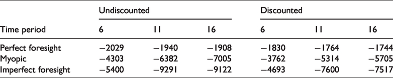
The figures are given in millions of pounds in 2010 prices and give a fuller quantitative indication of the impact of investment decisions on the severity of the impact of negative regional economic shocks. They are also useful in that although in the long run all the models return to their initial equilibrium, there are cases in which GDP overshoots the original equilibrium trajectory after the recovery, such as in the perfect foresight case or where they cross the equilibrium line more than once before full convergence is achieved, such as with imperfect foresight. This makes it difficult to establish a point at which the recovery is completed and consequently to calculate the indices reported above.

Note that for the cumulative GDP loss, discounted or undiscounted, the ordering of the models is always the same, reinforcing the impressions given from the previous measures: the perfect foresight model produces the lowest value, followed by the myopic and then imperfect foresight cases. Second, the cumulated aggregate differences are substantial. The GDP reductions for the myopic and imperfect foresight models are never less than double the comparable figures for perfect foresight, and are often much greater. Third, these differences become larger with longer time periods over which the measures are taken. This reflects the long, thick tail that characterizes their adjustment paths. In the undiscounted myopic case the cumulated reduced GDP in periods 7–16 equals just over 60% of the cumulated impact for periods 1–6. For the imperfect foresight case it is almost 70%. That is to say, where firms’ investment decisions use these heuristics, much of the negative impact occurs after the shock has ended.

Conclusion

In introducing behavioural elements into a CGE model, we highlight the treatment of investment, which necessarily involves uncertain outcomes that occur over time. We replace the standard economic assumption of perfect foresight with decision-making using heuristics, bringing the analysis closer to behavioural and Keynesian perspectives. The simulations suggest that adopting different plausible assumptions over the way investment decisions are taken has a major impact on the simulated effects of a temporary demand shock.

Although this paper focuses primarily on the investment decision, behavioural economics also has insights into consumption decisions and the operation of the labour market. Here we have suggested non-maximizing interpretations of these aspects of the model, but we intend in the future to make more extensive adjustments in these areas. For consumption, this would include hyperbolic discounting and consumer inertia across heterogeneous household types. We report simulations with alternative wage-setting options elsewhere (see note 8), but wish to extend this analysis by interacting labour market conditions and migration with different exogenous shocks.

In terms of resilience, the simulation results reported here are restricted to the response to a very general temporary demand shock. In future work we wish to consider other investment heuristics and the resultant simulated evolution of regional economic activity tested against actual responses to exogenous demand shocks. We also want to study the impact of supply shocks and investigate the way in which endogenous efficiency improvements could generate path dependency and hysteresis effects in ecological and evolutionary resilience settings. Finally, similar simulations should be performed to study the sensitivity of resilience to other regional characteristics that are thought to affect it. These would include industrial structure, regional openness, labour market flexibility, including wage setting and migration behaviour, and alternative fiscal rules.

Supplemental Material

sj-pdf-1-epn-10.1177_0308518X20941775 - Supplemental material for Resilience in a behavioural/Keynesian regional model

Supplemental material, sj-pdf-1-epn-10.1177_0308518X20941775 for Resilience in a behavioural/Keynesian regional model by Grant Allan, Gioele Figus, Peter G. McGregor and J. Kim Swales in Environment and Planning A: Economy and Space

Footnotes

Acknowledgements

The authors would like to thank participants at the Regional Science Association (British and Irish Section) Annual Conference, Harrogate, 2017, the 58th Congress of the European Regional Science Association, Cork, 2018 and the Brown Bag seminar of the Department of Economics, University of Strathclyde, 2018, for valuable comments on earlier versions of this paper. The authors are thankful for the useful comments of three anonymous referees.

Declaration of conflicting interests

The author(s) declared no potential conflicts of interest with respect to the research, authorship and/or publication of this article.

Funding

The author(s) received no financial support for the research, authorship and/or publication of this article.

ORCID iD

Gioele Figus

Notes

References

Akerlof

Shiller

(2009) Animal Spirits: How Human Psychology Drives the Economy and Why It Matters for Global Capitalism. Princeton: Princeton University Press.

Angner

(2012) A Course in Behavioral Economics. Basingstoke: Palgrave Macmillan.

Audit Scotland (2016) Scotland’s New Financial Powers: Key Issues for the Scottish Public Finances. Edinburgh: Audit Scotland.

Becker

(1976) The Economic Approach to Human Behaviour. Chicago: University of Chicago Press.

Blanchflower

Oswald

(2005) The wage curve reloaded. NBER Working Paper 11338, National Bureau of Economic Research, Cambridge, MA, USA.

Boeters

Savard

(2011) The labour market in CGE models. Discussion Paper 11-079, ZEW Centre for European Economic Research, Mannheim.

Cartwright

(2011) Behavioural Economics. London: Routledge.

Davoudi

(2012) Resilience: A bridging concept or a dead end? Planning Theory and Practice 13: 299–333.

Di Pietro

Lecca

Salotti

(2020) Regional economic resilience in the European Union: A numerical general equilibrium analysis. JRC Working Papers on Territorial Modelling and Analysis 03/2020, European Commission, Seville.

10.

Dixon

Jorgenson

(2013) Handbook of Computable General Equilibrium Modelling. Amsterdam: Elsevier.

11.

Dixon

Pearson

Picton

, et al. (2005) Rational expectations for large CGE models. Economic Modelling 22: 1001–1019.

12.

Earle

Moran

Ward-Perking

(2017) The Econocracy: The Perils of Leaving Economics to the Experts. Manchester: Manchester University Press.

13.

Eyal

Hoover

(2014) Hooked: How to Build Habit Forming Products. London: Penguin.

14.

Friedman

(1953) The methodology of positive economics. In: Essays in Positive Economics. Chicago: University of Chicago Press, pp.3–43.

15.

Friedman

(1993) The ‘plucking model’ of business fluctuations revisited. Economic Inquiry 31: 171–177.

16.

Galvez

(2014) Estimating a wage curve for the United Kingdom. MSc Dissertation, Scottish Graduate Programme in Economics, University of Edinburgh, UK.

17.

Gibson

(1990) Export competitiveness and UK sales of Scottish manufacturers. Working Paper, Scottish Enterprise, Glasgow, UK.

18.

Gilovich

Tversky

Vallone

(1985) The hot hand in basketball: On the misperception of random sequences. Cognitive Psychology 17: 295–314.

19.

Harcourt

(1995) Joan Robinson, 1903–1983. Economic Journal 105: 1228–1243.

20.

Harford

(2017) The problem with facts. Financial Times, 11–12 March.

21.

Harrassova

(2018) Estimating the elasticity of substitution between capital and labour. MSc Dissertation, Scottish Graduate Programme in Economics, University of Edinburgh, UK.

22.

Harrigan

McGregor

Dourmashkin

, et al. (1991) AMOS: A macro-micro model of Scotland. Economic Modelling 8: 424–479.

23.

Harris

(1989) The Growth and Structure of the UK Regional Economy (1963–1985). Aldershot: Avebury.

24.

Hausman

(1992) The Inexact and Separate Science of Economics. Cambridge: Cambridge University Press.

25.

HM Treasury and HM Revenue and Customs (2014) Analysis of the dynamic effects of fuel duty reductions. available online at https://www.gov.uk/government/publications/analysis-of-the-dynamic-effects-of-fuel-duty-reductions

26.

Holling

(1973) Resilience and stability of ecological systems. Annual Review of Ecological Systems 4: 1–23.

27.

Holling

(1996) Engineering resilience versus ecological resilience. In: Schulze

(ed.) Engineering within Ecological Constraints. Washington, DC: National Academy Press, pp.31–44.

28.

Kahneman

(2012) Thinking, Fast and Slow. London: Penguin.

29.

Keefe

(2017) Empire of Pain. New Yorker, 30 October, pp.34–49.

30.

Keynes

(1936) The General Theory of Employment, Interest and Money. London: Macmillan.

31.

Kwak

(2017) Economism: Bad Economics and the Rise of Inequality. New York: Pantheon.

32.

Laibson

(1996) Hyperbolic discount functions, undersaving, and saving policy. NBER Working Paper 5635, National Bureau of Economic Research, Cambridge, MA, USA.

33.

Layard

Nickell

Jackman

(2005) Macroeconomic Performance and the Labour Market. Oxford: Oxford University Press.

34.

Lecca

McGregor

Swales

(2013) Forward-looking and myopic regional computable general equilibrium models: How significant is the distinction? Economic Modelling 31: 160–176.

35.

Lewis

(2017) The Undoing Project. London: Allen Lane.

36.

Loewenstein

Prelec

(1992) Anomalies in intertemporal choice: Evidence and an interpretation. The Quarterly Journal of Economics 107: 573–597.

37.

Loewenstein

Schkade

(1999) Wouldn’t it be nice? Predicting future feelings. In: Kahneman

Diener

Schwartz

(eds) Well-Being: The Foundations of Hedonic Psychology. New York: Russell Sage Foundation.

38.

McLachlan

Swales

(1990) Friedman’s methodology: A comment on Boland. Journal of Economic Studies 9: 19–34.

39.

Malakellis

(1997) Should tariff reductions be announced? An intertemporal computable general equilibrium analysis. Preliminary Working Paper OP-88, Centre of Policy Studies/IMPACT Project, London, UK. Available at: http://www.copsmodels.com/ftp/workpapr/op-88.pdf.

40.

Martin

(2012) Regional economic resilience, hysteresis and recessionary shocks. Journal of Economic Geography 12: 1–32.

41.

Martin

Sunley

(2015) On the notion of regional economic resilience: Conceptualisation and explanation. Journal of Economic Geography 15: 1–42.

42.

Martin

Sunley

Gardiner

, et al. (2016) How regions react to recessions: Resilience and the role of economic structure. Regional Studies 50: 561–585.

43.

Pech

Milan

(2009) Behavioural economics and the economics of Keynes. Journal of Socio-Economics 38: 891–902.

44.

Robinson

(1960) Exercises in Economic Analysis. London: Macmillan.

45.

Robinson

(1962) Economic Philosophy. London: Penguin Books.

46.

Rodrik

(2016) Economics Rules: The Rights and Wrongs of the Dismal Science. New York: Norton.

47.

Rose

(2004) Defining and measuring economic resilience to disasters. Disaster Prevention and Management 13: 307–314.

48.

Rose

(2006) Macroeconomic impacts of catastrophic events: The influence of resilience. In: Berkeley symposium on real estate, catastrophic risk and public policy, University of California Berkeley, Berkeley, USA, 22–23 March 2006.

49.

Rose

Liao

(2005) Modeling regional economic resilience to disasters: A computable general equilibrium analysis of water service disruption. Journal of Regional Science 45: 75–112.

50.

Rosling

(2018) Factfulness. London: Sceptre.

51.

Simmie

Martin

(2010) The economic resilience of regions: Towards an evolutionary approach. Cambridge Journal of the Regions, Economy and Society 3(1): 27–43.

52.

Taylor

(2011) CGE applications in development economics. Working Paper, Schwartz Center for Economic Analysis and Department of Economics, New York, USA.

53.

Thaler

(2015) Misbehaving: The Making of Behavioural Economics. London: Penguin.

54.

Walker

Gunderson

Kinzig

, et al. (2006) A handful of heuristics and some propositions for understanding resilience in social-ecological systems. Ecology and Society 11(1): art. 13.

55.

Wei

Rose

Shantong

, et al. (2018) Dynamic economic resilience and economic recovery from disasters: A quantitative assessment. Risk Analysis 38: 1306–1318.

56.

Weimann

Knabe

Schob

(2015) Measuring Happiness: The Economics of Wellbeing. Cambridge, MA: MIT Press.

57.

Wren-Lewis

(2015) Unravelling the new classical counter revolution. Review of Keynesian Economics 4: 20–35.

58.

Wren-Lewis

(2018) Ending the microfoundations hegemony. Oxford Review of Economic Policy 34: 55–69.

Supplementary Material

Please find the following supplemental material available below.

For Open Access articles published under a Creative Commons License, all supplemental material carries the same license as the article it is associated with.

For non-Open Access articles published, all supplemental material carries a non-exclusive license, and permission requests for re-use of supplemental material or any part of supplemental material shall be sent directly to the copyright owner as specified in the copyright notice associated with the article.

0.00 MB

0.30 MB