On the origin of the ground effect

Abstract

The ground effect is well known to pilots and aerodynamicists alike. However, the current explanations found in undergraduate (and pilot-focused) textbooks can be inconsistent, often attributing the phenomena to the interaction between tip vortices at the ground. Others invoke the method of images to show that, when the flow is forced to have a straight streamline on the ground, ground pressure must increase. These must prescriptively choose an airfoil circulation. Meanwhile, a simple panel code can be used to show both that the lift on an airfoil in ground effect is significantly two-dimensional, and that the circulation about an airfoil near the ground is not constant. In particular, circulation will be found to grow as altitude decreases, magnifying the ground effect. A simple graphical panel method solver is provided, such that this exercise is accessible to students without the longer task of writing a panel code for themselves. This exercise can provide students with greater insight into the Kutta condition, the method of images, and panel methods themselves. The resulting streamline pattern can also be used to explain the phenomenon to more general audiences, by observing the relationship between lift and streamline curvature.

Introduction

Learning a wildly incorrect explanation for lift is an almost universal experience for children. Babinsky ¹ observed how a quick and seemingly logical explanation can gain popularity, even if it happens to be wrong, and even if it ultimately confuses students. This incorrect explanation, of course, is the ‘equal transit time’ argument: a parcel of fluid has to go farther ‘above’ an airfoil than ‘below’, and therefore it must move faster. Invoking Bernoulli’s equation, this faster flow must have lower pressure, and therefore there is a pressure difference across an airfoil – an explanation that is still found in many textbooks [see Illman ² ]. While lift does manifest through the pressure field, and Bernoulli’s equation can compute this pressure, parcels of fluid do not take an equal time to transit above and below an airfoil, and even as robust an equation as Bernoulli’s cannot account for an incorrect input. Meanwhile, a physically and logically sound explanation, as demonstrated by Babinsky, requires only a knowledge of streamlines, Newton’s second law, and the concept of centripetal force. Such an explanation is likely accessible to secondary students, especially as there is no need to go into the mathematical details of the streamline, as you would for undergraduates.

The ground effect has an analogous problem. Both pilots and aerodynamicists are familiar with the ground effect, in which an aircraft, wing or airfoil at low altitudes experiences increased lift. To pilots, this gives a floating sensation, or a feeling of reduced drag [see Federal Aviation Administration, ³ Ch 5–12]. To characterize the ground effect by ‘sensation’ is perfectly reasonable here, as the critical information in the piloting context is how the pilot can recognize and react to the phenomenon, rather the fluid mechanics. Some pilot information, however, attributes the phenomenon to the interaction between tip vortices and the ground [see Federal Aviation Administration, ³ Ch 5–11]. This same argument also appears in engineering texts [see Anderson ⁴ , p. 460]. So the explanation goes, as wingtip vortices produce induced drag, and reduce lift, the interruption of wingtip vortices by the ground alleviates both of these issues. If we compare classical models for the lift of an airfoil with and without tip vorticies, three-dimensional lifting-line theory and two-dimensional thin airfoil theory respectively, we might describe this explanation as:

$$C_L=2\pi \alpha \left(\frac{AR}{AR+2}\right)\to C_L=2\pi \alpha ,$$

(1)

where $C_L$ is the lift coefficient, $\alpha$ is the angle-of-attack, and $AR$ is the aspect ratio of the wing. ⁵ This explanation, though common, has two major problems: First, it prescribes an upper bound on the lift enhancement that the ground effect can produce, never exceeding $C_L=2\pi \alpha$ ; and second, it implies that the ground effect is a fundamentally three-dimensional phenomena. However, empirical observation shows that lift in ground effect substantially exceeds that predicted by thin airfoil theory, such that the absence of tip vortices is insufficient to explain the increase in lift. ⁶

Likewise, we can show that the ground effect is not three-dimensional either. The increase in velocity above an airfoil, and the decrease in velocity below it, is often modelled by the superposition of a free-stream flow with a vortex, as in potential flow. Integrating the pressure field about this vortex results in the classical Kutta-Joukowski lift theorem:

$$L=\rho U_{\mathrm{\infty }}\mathrm{\Gamma },$$

(2)

where $L$ is lift, $\rho$ is the density of the air, $U_{\mathrm{\infty }}$ is the velocity of the free-stream flow, and $\mathrm{\Gamma }$ is the strength of the vortex. This solution is found in any undergraduate aerodynamic text, such as Anderson, ⁷ although sign convention frequently varies. Using the method of images, we can extend this model to account for a nearby wall, such as the ground. We first model an airfoil as a vortex just as we had before, but then we mirror the domain about the line we wish to interpret as the ‘wall’, as shown in Figure 1. In order for the flow to be symmetric, this mirroring axis must be a streamline. As we have no viscous boundary condition in potential flow, we can interpret this streamline as a solid wall, and we can then integrate the pressure about either vortex to determine lift, yielding:

$$L=\rho U_{\mathrm{\infty }}\mathrm{\Gamma }+\frac{1}{4\pi }\frac{1}{h}\rho {\mathrm{\Gamma }}^2,$$

(3)

Figure 1.

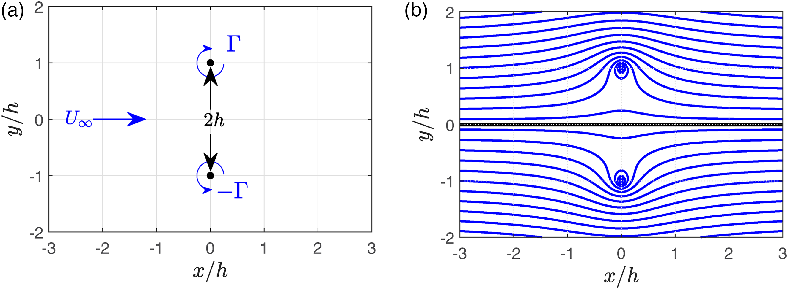
The potential flow of two equal but opposite vortices mirrored about an axis, shown left, produces a series of streamlines including one streamline along the mirroring axis, shown right. As no flow crosses a streamline, this line may be interpreted as a solid wall, neglecting viscosity.

where a new second term appears, as a function of $h$ , the altitude of the vortex above the ground. This approach, although less common, does appear in some aerodynamic textbooks such as Bertin, ⁸ and is routinely found in journal articles concerning the ground effect, such as Rayner and Bone. ⁹

In equation (3), we see that the lift coefficient is not bounded as the tip vortex explanation suggests, but is in fact singular as altitude approaches zero. However, what this model lacks is a relationship between the circulation $\mathrm{\Gamma }$ and the properties of the airfoil, especially angle of attack $\alpha$ . In thin airfoil theory, this relationship is determined by the Kutta condition, the condition that the circulation about an airfoil must be sufficient to maintain smooth flow from the trailing-edge. However, the analytical treatment of the Kutta condition is much more difficult when we have multiple airfoils, such as if we used the method of images to model the ground effect. We can address this limitation with a numerical solution using a panel method, which is an exercise accessible to undergraduates. The exercise can provide aerodynamics students insights into the Kutta condition, the ground effect, and potential flow. Moreover, we can use a visual inspection of the resulting streamlines to produce a more intuitive explanation of the origin of the ground effect, suitable for non-specialists in aerodynamics. Therefore, the purpose of this work is to provide software and a contextual framework to investigate the ground effect as a case study. In addition to the ground effect itself, this particular case study permits students to investigate several aerodynamics concepts including the Kutta condition, thin airfoil theory, potential flow, and panel methods in an accessible way by attempting to keep mathematical analysis as simple as possible. Moreover, by providing a means to ‘experiment’ with a concept before introducing a theory, it is hoped that students can experience the hypothesis-test methodology in a cost-effective manner.

A primer on a panel method exercise

In classical airfoil theory, circulation is distributed continuously along an airfoil’s surface. There is only one unique circulation distribution that simultaneously satisfies both the Kutta condition, and the requirement of no flow through the airfoil. By the mid-1950s, extensions to this basic idea were able to content with viscous effects, unsteady flows, and three-dimensional wings [see: Sears ¹⁰ ]. However, for many practical problems it is often easier to discretize the circulation rather than attempting to find a continuous analytical solution. This forms a class of techniques known as panel methods.

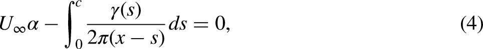
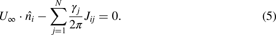
Many excellent textbooks already detail processes and procedures to compute panel method solutions, such as Cebeci et al., ¹¹ and so the description here will be significantly abridged. In short, the geometry of an airfoil can be discretized into a number of line segments called panels, and each panel is assigned a constant, but unknown, circulation. With a constant circulation along each panel, this circulation can be factored out of any integral across the geometry of the airfoil. And so, whereas thin airfoil theory solves an integral problem of finding a continuous circulation distribution as:

$$U_{\mathrm{\infty }}\alpha -{\int }_0^c\frac{\gamma (s)}{2\pi (x-s)}ds=0,$$

(4)

where $\gamma$ is circulation per unit length (i.e., where the circulation from equation (2) is distributed around the surface of an airfoil), panel methods are reduced to a mere algebraic problem, albeit of very similar form:

$$U_{\mathrm{\infty }}\cdot \widehat{n_i}-\sum _{j=1}^N\frac{{\gamma }_j}{2\pi }{J}_{ij}=0.$$

(5)

Here, equation (5) governs the flow on one panel $i$ , and $J_{ij}$ is a matrix whose elements are coefficients of influence between panels $j$ and $i$ , determined from the airfoil geometry. Highlighting this similarity often helps demonstrate that both equations are attempting to solve the same physics. For a sufficient number of panels, a solution arbitrarily close to thin airfoil theory can be obtained, as shown in Figure 2.

Figure 2.

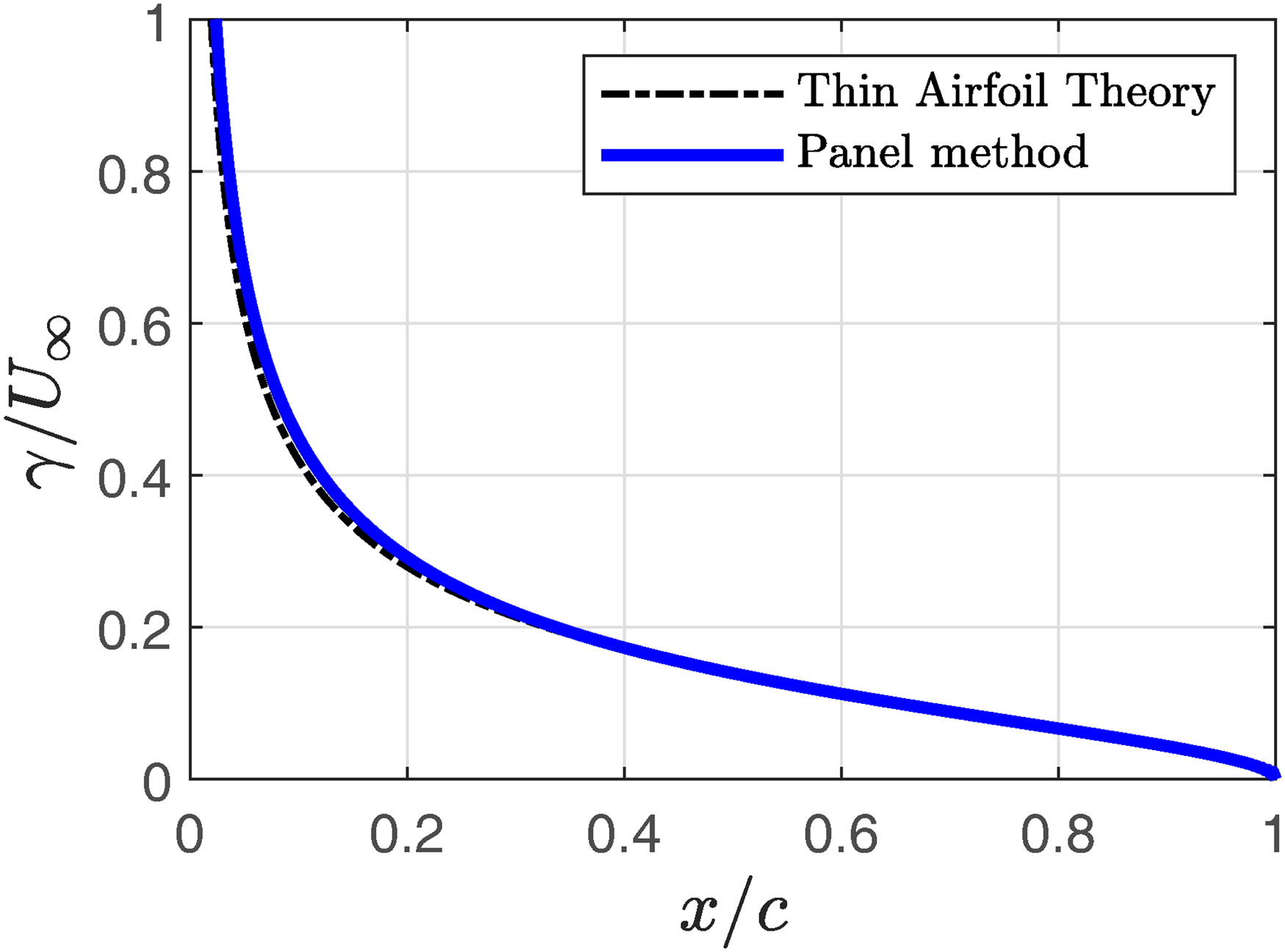
The circulation distribution of a panel satisfies the expected value from thin airfoil theory. The angle of attack is taken as $\alpha =4^{\circ }$ in both cases.

Outside of longer term-length projects, producing a complete panel method code is a difficult project even for senior undergraduates. Unless the purpose of the course is to investigate numerical methods, the same aerodynamic insight can usually be obtained by providing students with sample codes. Depending on specific course objectives, this can take many forms, such as:

A complete sample code for a single airfoil is provided, and students are asked to mirror the airfoil to simulate the ground effect,

a partial sample code for both a primary and mirror airfoil is provided, and students are asked to complete it (e.g., modifying it to enforce the Kutta condition),

a complete pseudo-code is provided that students must implement, or

a complete code is provided for students to investigate through play,

A GUI-based code suitable for the fourth option is included in the supplementary materials, implemented in MATLAB. The code is an adaptation of a methodology found in Kuethe and Chow. ¹² Please note that this sample code is meant to be fast and illustrative foremost, and sacrifices accuracy somewhat in these goals. Using this example, students can be asked questions related to simple airfoil theory, such as being tasked to independently discover the lift slope from thin airfoil theory, or they could simultaneously or separately investigate how the numerical implementation of the Kutta condition relates to the observed aerodynamic phenomenon. Modifying the problem for the ground effect, a student could be asked to find different lift slopes at various altitudes, or to discuss how the method of images enables the analysis.

Expected exercise results

Lift curves produced by the provided example code is shown in Figure 3 for several altitudes. The lift coefficient predicted here at an angle of attack of $\alpha =1/2\pi$ is slightly higher than the expected value of one. Or in other words, the lift slope is approximately 2% higher than the $2\pi$ expected from thin airfoil theory. However, the accuracy here is likely sufficient for most classroom applications, and it should be noted that the code was written with the intention that students could attempt to parse the methodology. Furthermore, a significant delay between button press and the presentation of a plotted flow solution was to be avoided, as it could be an obstacle to student interactivity.

Figure 3.

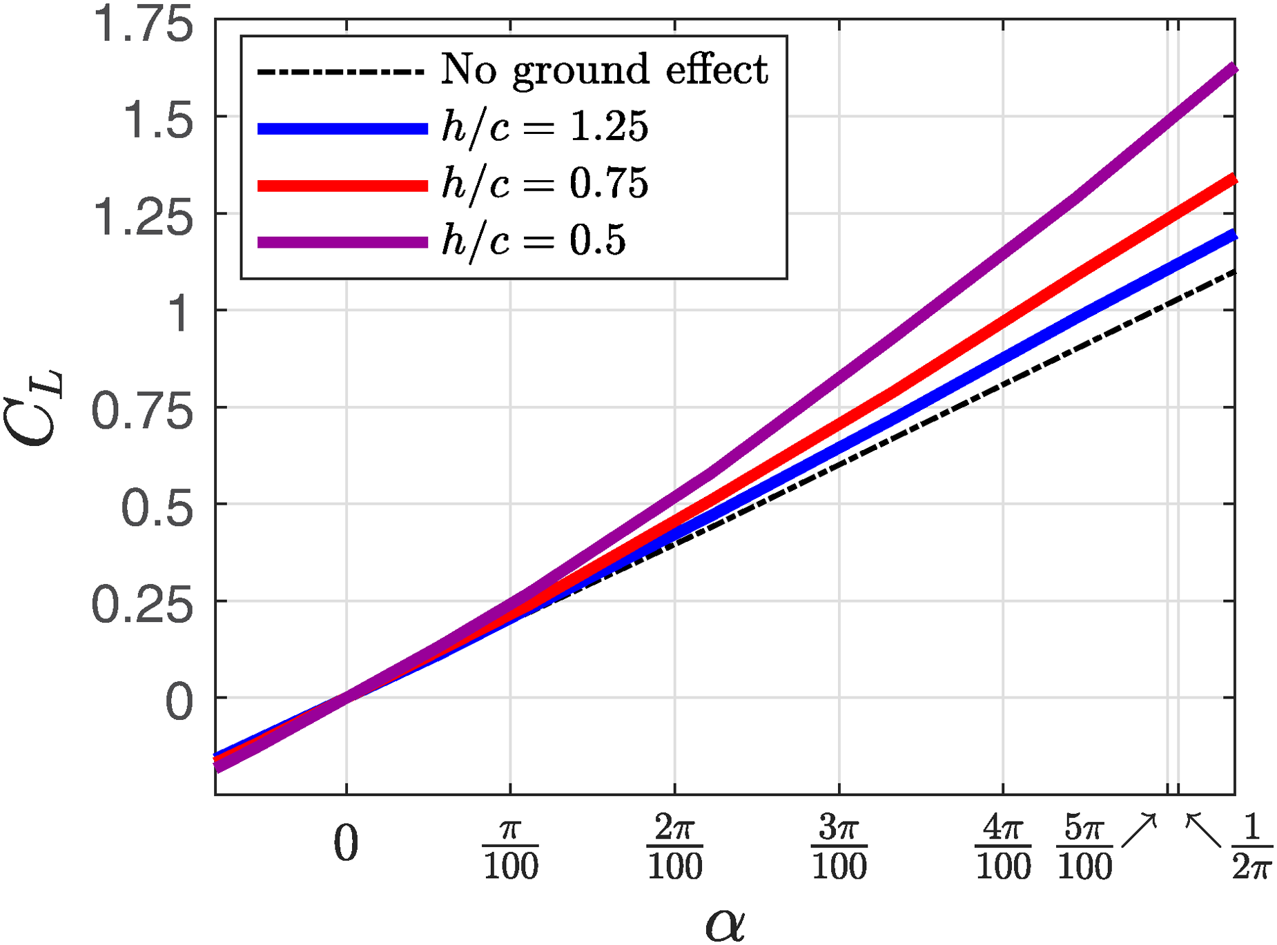
The lift coefficient estimated by a panel code at various altitudes. The $1/2\pi$ marker is included to quickly estimate the lift slope.

A curve-fitting exercise shows that lift is parabolic with angle of attack for each of the ground effect cases ( $R^2>0.9995$ ), which is exactly what one would expect from equation (3) if we assume that circulation grows proportionally to angle of attack, as it does in thin airfoil theory. However, we can not yet say that circulation is a function of angle of attack alone.

If we assume a constant circulation, we can predict lift as a function of altitude with equation (3), by imposing a no-normal-flow condition at the ground. Taking $\mathrm{\Gamma }/U_{\mathrm{\infty }}c=\pi \alpha$ , as we would for thin airfoil theory, we can plot lift as a function of altitude. We can plot a similar relationship for lift versus altitude at the same time using a panel code. An example of this is shown in Figure 4, for $\alpha =4^{\circ }$ . Here, lift significantly exceeds the value predicted by a constant circulation, especially at low altitudes. Therefore, we can conclude that the bound circulation is varying with both altitude and angle of attack.

Figure 4.

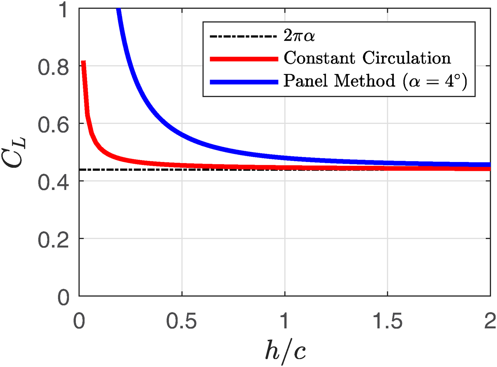
The lift coefficient of a flat plate at various altitudes exceeds the value preducted by a constant circulation.

For a student, this can be used to illustrate the primacy of the Kutta condition. The panel method is only explicitly enforcing two physical conditions: there is no flow through the airfoil, and there is smooth flow from the trailing-edge. The third boundary condition, that there is no flow normal to the ground, is enforced implicitly through the symmetry of the domain. As there are infinitely many integral values of circulation that satisfy the no normal flow condition, we can therefore conclude that this result in the ground effect can only be explained through the Kutta condition. This may further help a student appreciate that the results they found previously, when investigating thin airfoil theory, are of a more general class of airfoil flows rather than ‘the’ solution.

The distribution of circulation at different altitudes is shown in Figure 5. While it may appear at first glance as if the difference in circulation between ground effect cases and thin airfoil theory is concentrated in the midsection of the airfoil, this is due to the large slope of the circulation curve masking the difference between the curves. When they are subtracted, as in Figure 5(b), we see that the difference is concentrated near the leading edge, with half of the difference in circulation occurring before the quarter chord. The leading-edge circulation is associated with the flow wrapping around the leading-edge of the airfoil. A similar peak in circulation appears for finite thickness wings, albeit with a finite magnitude. As such, this peak is associated with the location of the location of the stagnation streamline, which provides an alternative and possibly more intuitive explanation for the ground effect based on streamline curvature.

Figure 5.

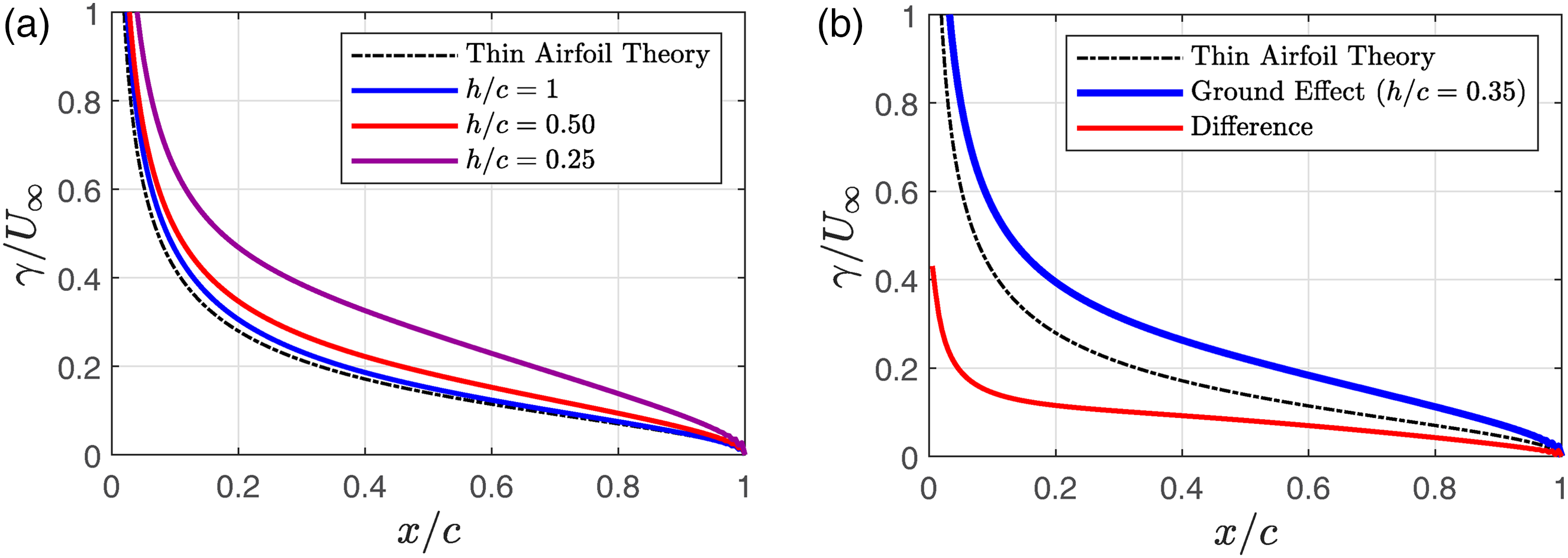
The bound circulation grows as altitude decreases (a). Due to the singular nature of the bound circulation, the difference may appear to concentrate in the middle of the airfoil. However, the difference is concentrated strongly towards the leading-edge (b).

Streamlines computed by the sample code are shown in Figure 6. As the altitude decreases, the stagnation streamline intersects the wing further back from the leading-edge. Specifically, as altitude shrinks from infinity to $h/c=0.25$ , the distance of the stagnation point from the leading edge doubles, from $x/c=0.0064$ to $x/c=0.0131$ . This shift in stagnation streamline has been observed by Ahmed et al. ¹³ in wind tunnel experiments. The shift in stagnation streamline coincides with an increase in streamline curvature, especially about the leading-edge.

Figure 6.

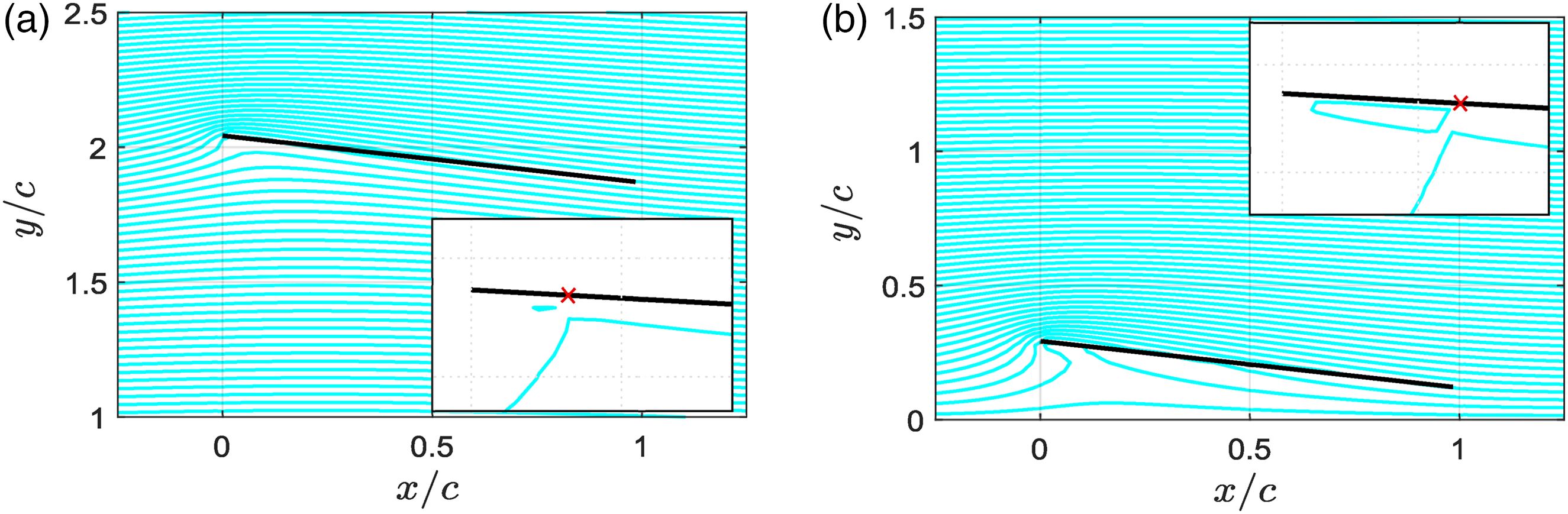
The streamlines show that the stagnation point for (a) $h/c=2$ shifts away from $x/c=0.0064$ to (b) $x/c=0.0131$ when the altitude decreases to $h/c=0.25$ .

A more intuitive explanation for the ground effect

To explain the lift on an airfoil, Babinsky ¹ observed the streamlines about an airfoil and noted the increase in curvature above the airfoil. In the same way that a weight spun in a circle on a string requires the tension of the string to enforce its circular path, there must be a force to curve a streamline, towards the centre of curvature. In a fluid, that force manifests through the pressure field. And therefore, if there is concave-down streamline curvature above an airfoil, and it is atmospheric pressure far from the airfoil, it stands to reason the airfoil surface would be a pressure minimum. A similar process was used to argue that the lower surface must be a pressure maximum. Babinsky then concludes that streamline curvature is associated with lift.

Depending on the background knowledge and age of the audience, or the instructional context, it may not be necessary to discuss why the pattern of streamlines appears as it does. For example, a discussion of lift at the secondary level, or in a museum targeting a general audience, can omit major aspects of flow development, such as boundary layer properties or the Kutta condition. From there, as long as it is established that the pattern of streamline curvature appears, we can explain lift. Certainly most educators would agree that a correct, logically consistent, but incomplete explanation is preferable to a complete but misleading one.

The ground effect may benefit from a similar strategy in certain contexts, for example in literature targeting pilots, or junior-level undergraduate classes that may want to mention the phenomenon without rigorously analysing it. The shift in the leading-edge stagnation streamline, and the coinciding increase in streamline curvature, follows logically from the discussion above of lift on airfoils in general. Moreover, this increased curvature can be visualized from vortices in potential flow (e.g., as in Figure 1(b)), panel methods (e.g., as in Figure 6), or from wind tunnel or CFD visualizations, such that a presenter can rely on the empirical fact of its appearance rather than attempting to justify it from physical reasoning.

Classroom experiences

The MATLAB app described above was provided to students taking the senior Aerodynamics course at the University of Alberta. In addition, the lectures that introduced the topics of thin airfoil theory, the ground effect, and panel methods, respectively were each modified to begin with fifteen to twenty minute exercise of investigating the problems ‘empirically’ using the provided software. Due to limited ethics approvals, only qualitative descriptions are presented here, and therefore primarily represent the instructor’s experience rather than pupils’.

Before introducing thin airfoil theory, a linear plot of lift versus angle of attack was generated, confirmed to be linear by curve fitting, and then students were asked to hypothesize why that particular function (versus, say, a quadratic or exponential function) might result, and why a symmetric airfoil (in this case, a flat plate) produced lift, contrary to primary-school explanations. Likewise, before introducing the ground effect, quadratic plots were generated, confirmed to be quadratic by curve fitting, and students were asked to hypothesize why that may result, versus the linear function of thin airfoil theory. After this, the appropriate theory was introduced as it was in prior terms, and the student’s hypotheses were revisited thereafter. Qualitatively, students appeared to appreciate this approach: participation in discussion were engaged, and students tended to ask more fundamental questions (rather than clarifying questions) than previous terms. Classroom attendance tended to increase for discussion-based lectures, and seemed to clarify the motivation for going into the theory.

Conclusion

Existing treatment of the ground effect in both aerodynamics classes at the university level, and in pilot instruction, is inconsistent, and often relies on the role of tip vortices. A treatment of the phenomenon using simple vortices with the method of images accurately describes the increase in lift at low altitudes for a given circulation, but stops short of discussing the relationship between circulation and altitude. A panel method solver is provided here to explore the behaviour of an ideal flat-plate airfoil in the ground effect. Investigating the ground effect in this way, students have the opportunity to independently re-discover the lift slope provided by thin airfoil theory, to verify the relationship between circulation and lift estimated using the method of images, and to observe the Kutta condition behaving as a general principle rather than as a specific case. Optionally, they may investigate the application of panel methods as an exercise on the technique, or at more senior levels, possibly write their own. Lastly, the exercise provides an opportunity for critical analysis of literature, as a student may be given the task of evaluating explanations found throughout the literature, and if they can or cannot be made to reconcile with their own observations.

The lift predicted by inviscid methods exceeds that predicted by wind tunnel measurements or CFD [see: Ahmed et al., ¹³ and Li et al. ¹⁴ ]. However, many general observations are consistent between both ideal flow and viscous flow: The leading-edge stagnation streamline moves downstream, increased streamline curvature appears near the leading-edge, and lift increases. These observations are sufficient to explain the ground effect without invoking three-dimensionality or the role of tip vortices, if the audience is willing to accept the pattern of streamlines in the flow, and especially if they have already been primed with a relationship between streamline curvature and lift. Such an explanation may be accessible to junior-level undergraduates, pilot instruction, and possibly even more general audience if required.

Supplemental Material

sj-docx-1-ijj-10.1177_03064190231174438 - Supplemental material for On the origin of the ground effect

Supplemental material, sj-docx-1-ijj-10.1177_03064190231174438 for On the origin of the ground effect by Lisa Long and Jaime G Wong in International Journal of Mechanical Engineering Education