Sage Journals: Discover world-class research

Abstract

Perceiving facial attractiveness is an important behaviour across psychological science due to these judgments having real-world consequences. However, there is little consensus on the measurement of this behaviour, and practices differ widely. Research typically asks participants to provide ratings of attractiveness across a multitude of different response scales, with little consideration of the psychometric properties of these scales. Here, we make psychometric comparisons across nine different response scales. Specifically, we analysed the psychometric properties of a binary response, a 0–100 scale, a visual analogue scale, and a set of Likert scales (1–3, 1–5, 1–7, 1–8, 1–9, 1–10) as tools to measure attractiveness, calculating a range of commonly used statistics for each. While certain properties suggested researchers might choose to favour the 1–5, 1–7 and 1–8 scales, we generally found little evidence of an advantage for one scale over any other. Taken together, our investigation provides consideration of currently used techniques for measuring facial attractiveness and makes recommendations for researchers in this field.

Keywords

face perception facial attractiveness response scale psychometric

First impressions based on facial appearance are formed rapidly (Willis & Todorov, 2006), without awareness (Olson & Marshuetz, 2005), and are mandatory (Ritchie et al., 2017). The nature of these impressions can have a substantial impact on how we subsequently behave towards others. For instance, individuals who appear less trustworthy may receive harsher criminal sentences (Wilson & Rule, 2015) while those who are perceived to be more competent have a greater likelihood of success in political elections (Ballew & Todorov, 2007). Attractiveness in particular plays an influential role in our first impressions, with the ‘halo effect’ (Dion et al., 1972) describing how socially desirable traits are applied indiscriminately to attractive people. As a result, being attractive comes with numerous benefits. For example, attractive people are given more help (Benson et al., 1976), earn higher wages (Pfeifer, 2012) and enjoy more frequent hiring opportunities (López Bóo et al., 2013). It also follows that attractiveness influences mating success (Rhodes et al., 2005). Given the significance of perceived attractiveness on a variety of real-world outcomes, it is unsurprising that researchers have been investigating these perceptions for many years. This, of course, then begs the question: how should perceived attractiveness be measured?

One approach is to measure perceptions of attractiveness implicitly, focussing on behavioural or physiological responses that are outside of conscious awareness. For instance, we tend to look longer and more often at attractive faces (e.g., Leder et al., 2016a, 2016b), they cause our pupils to constrict (Liao et al., 2021), and they capture our attention when presented outside foveal vision (Sui & Liu, 2009). Attractive faces also attract hand movements during mouse tracking paradigms (Faust et al., 2019) and we lean more towards them during passive viewing (Kramer et al., 2020). Finally, both brain activity (e.g., Ueno et al., 2014; Winston et al., 2007) and skin conductance (McDonald et al., 2008) have been shown to reflect our perceptions of facial attractiveness. Although these techniques might be considered more direct measures of our perceptions in the sense that we are typically unaware of our responses, they often require additional equipment, logistical considerations, and expertise.

Perhaps the simplest way to measure attractiveness perceptions, and certainly the most prevalent in the literature, is to ask participants directly. This is often achieved by using a rating scale. Although typically presented in the form of a Likert scale (e.g., Kramer et al., 2013), this explicit judgement might also be represented as a visual analogue scale (VAS; e.g., Dourado et al., 2021; Hofmans & Theuns, 2008) or a binary choice (e.g., Taubert et al., 2016). For researchers who opt for a Likert scale, a decision must still be made as to the range of options available, for instance: 1–3 (e.g., Cooper et al., 2006; Ma, Xu, et al., 2015), 1–5 (e.g., Langlois & Roggman, 1990), 1–7 (e.g., Ma, Correll, et al., 2015; Penton-Voak et al., 2001; Rhodes et al., 2005; Sutherland et al., 2013), 1–8 (e.g., Pegors et al., 2015), 1–9 (e.g., Oosterhof & Todorov, 2008), or 1–10 (e.g., Kampe et al., 2001; Kramer et al., 2013). Other scales used in research have included −5 to +5 (e.g., Skrinda et al., 2014) and 0–100 (e.g., Kramer & Jones, 2022; Orghian & Hidalgo, 2020), although this list is far from exhaustive. The appeal of such scales is their ease of use, allowing them to be employed with children (e.g., Ma, Xu, et al., 2015) and those with intellectual disabilities (Donnachie et al., 2021). Rating scales are also well-suited for use with online data collection (e.g., Kramer & Pustelnik, 2021), which is not the case for many of the more direct measures of perception mentioned earlier. It is worth noting that other methods may provide more reliable measures of facial attractiveness perceptions (e.g., best-worst scaling; Burton et al., 2019, 2021) but, as yet, this has not impacted the widespread use of rating scales.

While little has been done in considering whether different scales affect outcomes for attractiveness perceptions, psychometricians have been comparing the use of scale types more generally for several decades (for a review, see Cox, 1980). To determine the optimum number of response categories, one must account for possible advantages and disadvantages. For instance, short scales with few response options may be too coarse when attempting to capture raters’ discriminative powers. In contrast, too many response options may go beyond the raters’ discriminative abilities while adding superfluous choices. Initially, researchers argued that 3-point scales were sufficient when measuring participants’ opinions with respect to reliability and validity considerations (e.g., concerning agreement with statements regarding values – Jacoby & Matell, 1971). However, others noted that the motivation for data collection is key – if the aim is to average responses across participants then 2- or 3-point scales are sufficient, while 5- to 7-point scales are required if the focus is to investigate individual behaviour (as demonstrated through the use of simulations; Lehmann & Hulbert, 1972). Although there are typically high correlations between ratings provided using different lengths of scale (e.g., when considering the quality of a recent service provider – Colman et al., 1997; when considering treatment goals following surgery – Lange et al., 2020), those with more response options tend to produce data more closely resembling a normal distribution (e.g., for a self-esteem questionnaire – Leung, 2011). In general, it seems that larger numbers of responses have the effect of improving both reliability and validity (for a survey measuring life satisfaction – Alwin, 1997; for measuring the quality of a service provider – Preston & Colman, 2000), although beyond seven options, this improvement is minimal (with simulated data – Lozano et al., 2008).

Investigations into how participants use response scales have revealed several different response styles that might be displayed. For instance, some people may tend to choose the most extreme responses while others may favour the more positive options of the scale (e.g., when considering agreement with attitudinal statements covering various topics – Baumgartner & Steenkamp, 2001). Through considering a survey measuring impulsive purchasing and comparing response scales ranging from four to nine points, alongside the use of eye tracking techniques, Chen et al. (2015) found that only the 6-point scale suffered from greater attention to the positive options, while the longer scales (7–9 points) showed evidence of participants attending more to the extreme responses. Further, the 5- and 7-point scales required the least cognitive effort (i.e., the shortest response times). Finally, evidence suggested that the inclusion of middle points (e.g., a 5- rather than 4-point scale) was beneficial in that their presence shifted response proportions away from the remaining options (with the assumption that utilised options provide additional information), with the added advantage of decreasing extreme response styles (Weijters et al., 2010). Interestingly, as the number of response options increased, the effect of removing the middle point decreased. Chen and colleagues concluded that, weighing up these advantages and disadvantages, their 5-point scale was optimal.

Another available option to researchers is the VAS, where participants can select any location along a line to represent their response. The idea is that VAS is more sensitive as a measure because of its small gradations, and responses using this type of scale have been shown to be linear (e.g., when measuring job satisfaction or the attractiveness of faces – Hofmans & Theuns, 2008). However, evidence suggests that VAS responses are strongly correlated with those produced using Likert scales, while users tend to prefer the latter due to their ease and simplicity (e.g., when measuring facial pleasantness – Dourado et al., 2021). Further, VAS may not provide any psychometric advantages beyond scales incorporating six or more response options (e.g., with personality questionnaires – Simms et al., 2019).

Considering further the notion that participants show preferences for some scales over others, Preston and Colman (2000) investigated lengths of scale ranging from 2 to 11 response options when participants were asked about the quality of a service provider. Participants judged the 5-, 7- and 10-point scales as the easiest to use. However, those rated as the quickest to use were those with the fewest options: 2-point, 3-point and 4-point scales. Finally, when considering which scales allowed the participants to express their feelings adequately, participants preferred the longest scales (9–11 response options). Overall, the researchers suggested that the most preferred scale length was 10 points, closely followed by the 7-point and 9-point scales.

While psychometricians have long debated the different characteristics of these various scales, researchers within the field of face perception have yet to give it consideration. As is clear from the literature, research on this topic spans a wide range of disciplines but there remains little overlap with considerations of facial attractiveness at present (e.g., Dourado et al., 2021). We therefore take the first steps in exploring the psychometrics of the various response scales used when judging facial attractiveness by investigating a variety of scale properties, including several measures of inter-rater agreement and within-person consistency, as well as quantifying shared versus private taste, all of which may vary depending on the number of available responses. We also focus on scale use, examining how often different response options are chosen, as well as face-level outcomes, by comparing how the attractiveness assigned to each face differs across response scales.

Method

Participants

A sample of 567 volunteers (362 women, 193 men, 10 nonbinary, 1 nonconforming, 1 preferred not to say; age M = 30.5 years, SD = 15.4 years; self-reported ethnicity: 3% Black, 4% Asian, 90% White, 3% Mixed or Other or preferred not to say) provided written, informed consent online before taking part, and received an onscreen debriefing upon completion of the experiment. Participants were recruited via student researchers as part of their ‘research skills’ module. This study was approved by the University of Lincoln's ethics committee (ref. 10146) and was carried out in accordance with the provisions of the World Medical Association Declaration of Helsinki.

The data from an additional 73 participants were excluded because these individuals either responded incorrectly to one or more attention checks (see below for details) or provided the same response for all images within a block. As such, we could be confident in the quality of our remaining data.

Stimuli

From a larger set of facial photographs featured in the Chicago face database (Ma, Correll, et al., 2015), we considered only the White models (93 men and 90 women). This allowed us to focus on response method while avoiding the additional influence on ratings due to the presentation of face sequences varying in ethnicity (e.g., Kramer et al., 2013). All individuals wore grey t-shirts and were photographed in colour, front-on, and posed with a neutral expression at a fixed distance from the camera.

Norming data for these images were provided alongside the database and included attractiveness ratings, given using a Likert scale (1 = not at all, 7 = extremely). From these 183 models, we selected a final set of 20 women (attractiveness M = 3.42, SD = 1.01) and 20 men (attractiveness M = 3.01, SD = 0.71) who evenly spanned the full range of attractiveness values represented by the initial set of images.

Procedure

The experiment was carried out using the Gorilla online testing platform (Anwyl-Irvine et al., 2020). Information was collected regarding the participant's age, gender and ethnicity. Participants were prevented from using mobile phones (via settings available in Gorilla) to ensure that images were viewed at an acceptable size onscreen.

Each participant judged all 40 images, presented in a random order, with the question ‘How attractive is this face?’ appearing at the top of the screen. Upon completion of this first block, participants were instructed onscreen that they were halfway through the task, and that they would see all of the faces again. At this point, participants were presented with all 40 images in a random order and again judged the attractiveness of the images. Both blocks were presented within the same condition (see below), and so judgements always followed the same response requirements for a given participant.

Participants were randomly assigned to one of ten conditions in which the available response requirements differed. Six of these conditions were Likert scales (1–3, 1–5, 1–7, 1–8, 1–9, 1–10), with labels displayed alongside the lowest (‘unattractive’) and highest (‘attractive’) values. The seventh condition required a binary response (unattractive/attractive), with only these two options (and no values) presented.

The eighth condition featured a 0–100 (i.e., 101-point) scale, where participants moved a slider along a line to select their response. The current position of the slider (a value from 0 to 100) was displayed onscreen, allowing participants to alter and refine their choice as needed before submitting their response. Labels were displayed alongside the left (‘unattractive’) and right (‘attractive’) endpoints of the line. Closely resembling this condition, the ninth condition was a VAS. The only difference between the 0–100 and the VAS conditions was that the latter did not display a value indicating the slider's position. As such, participants made their response based solely on the slider's visual position along the line. (Again, participants could alter and refine their choice before submission.) For both of these conditions, the line was initially presented without a slider, which then appeared as a result of the participant's first selection along the line (and could then be altered). As such, participants were not able to skip through trials by relying simply on the slider's default position (since there was no such position).

Finally, we included a ‘text response’ condition. Here, in addition to the question ‘How attractive is this face?’, participants were provided with the prompt ‘Describe your impressions of the attractiveness of this face’ and given a textbox in which to type their response. There was no limit placed on the length of response that could be entered. Participants completed only one block for this condition, given the longer time taken in comparison with simply rating the faces, and also that within-person agreement was not a consideration. For all ten conditions, responses were self-paced with no time limit.

In each block of images across all conditions, we also included an attention check within the randomly ordered presentation of faces, given that attentiveness is a common concern when collecting data online (Hauser & Schwarz, 2016). Each of these trials instructed the participant to respond with the lowest or highest option available for that condition. For instance, the text ‘Attention Check: Please respond with “9” for this face’ replaced the internal features of a face (not included in the 40 test faces) that was displayed onscreen. Across the two blocks, one attention check required the lowest response option available (e.g., ‘1’) and the other required the highest (e.g., ‘9’). For the attention check included in the single block for the ‘text response’ condition, participants were required to enter the word ‘house’ into the textbox as their response.

Results

The data from the 32 participants who completed the ‘text response’ condition will be the focus of a separate manuscript and will not be considered further here. The sample included in the following analyses therefore comprised 535 participants, with their trial-level response data available at https://osf.io/s8qp4/.

The measures of inter-rater agreement and within-person consistency presented here were, for the most part, also those investigated by Kramer et al. (2018). More information on each of these measures can be found in their article. In all cases below, Spearman's rank correlation coefficient was used as the measure of association. Following Kramer and colleagues, we have provided confidence intervals to illustrate the precision of our measures. For both measures of intraclass correlation, IBM SPSS Statistics v28 provided values for the 95% confidence intervals. However, for the remaining measures, there is no established method for obtaining interval estimates. We therefore used a bootstrapping procedure in MATLAB, over 10,000 samples with replacement, to estimate standard errors, and subsequently, confidence intervals.

We considered the binary response condition separately (see below) since our measures of inter-rater agreement and within-person consistency could not be calculated for this type of response.

Inter-Rater Agreement

Cronbach's α. Perhaps the most popular measure of inter-rater agreement is Cronbach's α (Cronbach, 1951). Although initially developed to quantify reliability in psychometric tests, it is also widely used within the social perception literature as a measure of reliability among raters (e.g., Oosterhof & Todorov, 2008). Problematically, however, since raters are treated as items, simply increasing the number of raters results in an increase in its value (Cortina, 1993). Another issue with this statistic is that a high Cronbach's α means only that the ratings given are capable of estimating those of the general population, but it does not follow that such judgements are mostly shared (Hönekopp, 2006). This is because Cronbach's α fails to consider the importance of within-person variability (i.e., how much raters agree with themselves).

Despite these criticisms, we calculated this measure for our scales to allow for comparison with each other, as well as with previous literature. As Table 1 illustrates, Cronbach's α was high for all scales and showed little variation.

Table 1.

A summary of measures for eight conditions regarding inter-rater agreement.

Condition	n	Cronbach's α	ICC(A,k)	Average ‘Leave One Out’	Kendall's W	Average inter-rater agreement
1–3 scale	64	0.97 [0.95, 0.98]	0.95 [0.93, 0.97]	0.56 [0.52, 0.60]	0.36 [0.27, 0.44]	0.31 [0.31, 0.32]
1–5 scale	61	0.98 [0.97, 0.99]	0.97 [0.95, 0.98]	0.65 [0.62, 0.68]	0.38 [0.28, 0.48]	0.43 [0.42, 0.44]
1–7 scale	63	0.98 [0.97, 0.99]	0.97 [0.95, 0.98]	0.70 [0.67, 0.73]	0.43 [0.33, 0.54]	0.49 [0.48, 0.49]
1–8 scale	66	0.98 [0.97, 0.99]	0.97 [0.96, 0.98]	0.69 [0.66, 0.72]	0.41 [0.29, 0.53]	0.47 [0.47, 0.48]
1–9 scale	61	0.98 [0.97, 0.99]	0.96 [0.93, 0.97]	0.69 [0.65, 0.72]	0.41 [0.30, 0.52]	0.47 [0.47, 0.48]
1–10 scale	58	0.97 [0.95, 0.98]	0.94 [0.91, 0.96]	0.63 [0.58, 0.67]	0.34 [0.21, 0.48]	0.39 [0.38, 0.40]
0–100 scale	60	0.98 [0.97, 0.99]	0.97 [0.95, 0.98]	0.71 [0.67, 0.74]	0.47 [0.33, 0.61]	0.50 [0.49, 0.51]
Visual analogue scale	49	0.97 [0.96, 0.99]	0.95 [0.93, 0.97]	0.69 [0.66, 0.73]	0.47 [0.35, 0.59]	0.49 [0.48, 0.50]

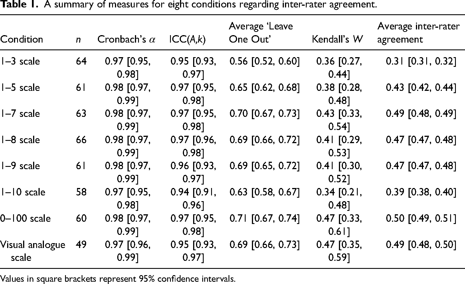
Values in square brackets represent 95% confidence intervals.

Intraclass correlation. We calculated the intraclass correlation coefficient, ICC(A,k), for each scale. While Cronbach's α, also termed ICC(C,k), ignores any absolute differences between raters (and only considers consistency), this version of the intraclass correlation coefficient takes such differences into account. In other words, consistent raters may agree on the general order of faces while differing in absolute ratings (e.g., one rater gives higher values than another). If the purpose of a study is to select faces which have been rated above or below a predefined absolute value, or to utilise their absolute (mean) value in some way, then raters must demonstrate absolute agreement for this to be meaningful. As Table 1 illustrates, mirroring the results with Cronbach's α, ICC(A,k) was high for all scales and showed little variation.

Average ‘leave one out’ correlation. For each participant, we correlated their ratings (given in the first block of the task) with the mean of the remaining participants (e.g., Bronstad & Russell, 2007; Germine et al., 2015; Zebrowitz et al., 2013). We then averaged these correlations together, producing a value where higher indicates greater agreement within the sample. Intuitively, this value represents how much we can expect a particular participant to agree with the rest of the group. Average correlations were calculated by first performing Fisher's r-to-z transformations, which correct for the skew in correlation distributions and provide an unbounded quantity that is approximately normal. The resulting z-values were then averaged, and we finally applied z-to-r transformations (Rosenthal, 2018). As Table 1 illustrates, there was some suggestion that this correlation increased with an increase in scale length. However, in all cases, correlations were large.

Kendall's W. This statistic (also known as the coefficient of concordance; Kendall, 1948; Kendall & Smith, 1939) is proportional to the average rank-order correlation among all pairs of raters, and so higher values demonstrate higher agreement (e.g., White et al., 2016). Again, as Table 1 illustrates, Kendall's W showed a slight increase with an increase in scale length.

Average inter-rater agreement. Finally, we considered the average inter-rater agreement (e.g., Bronstad & Russell, 2007; Hönekopp, 2006; Leder et al., 2016a, 2016b; Rezlescu et al., 2015). Simply, we calculated the correlation between every possible pair of raters and then averaged these values (using Fisher's transformations as above). As Table 1 illustrates, we found somewhat higher values with increasing scale length, although all values fell within the medium-to-large range of associations.

Within-Person Consistency and Shared/Private Taste

To quantify within-person consistency (i.e., test-retest reliability), we correlated each rater's responses given during the first block with those from the second block. These correlations were then averaged (using Fisher's transformations as above). For all scales, consistency was high, although it appears to decrease for scales with fewer response options (see Table 2). It is interesting to note that these high within-person correlations (0.72–0.79), alongside the substantially lower values for the average inter-rater agreement (0.31–0.50), suggest that private taste features heavily in these perceptions. While raters agreed strongly with themselves, their agreement with others was far lower.

Table 2.

A summary of measures for eight conditions regarding within-person consistency and shared/private taste.

Condition	n	Within-person consistency	Beholder index, bi₁
1–3 scale	64	0.72 [0.65, 0.77]	0.62 [0.54, 0.70]
1–5 scale	61	0.73 [0.69, 0.76]	0.52 [0.44, 0.59]
1–7 scale	63	0.74 [0.70, 0.77]	0.50 [0.42, 0.58]
1–8 scale	66	0.78 [0.75, 0.81]	0.49 [0.42, 0.57]
1–9 scale	61	0.75 [0.72, 0.78]	0.50 [0.41, 0.59]
1–10 scale	58	0.76 [0.70, 0.81]	0.58 [0.49, 0.68]
0–100 scale	60	0.78 [0.74, 0.81]	0.49 [0.41, 0.58]
Visual analogue scale	49	0.79 [0.75, 0.82]	0.51 [0.44, 0.59]

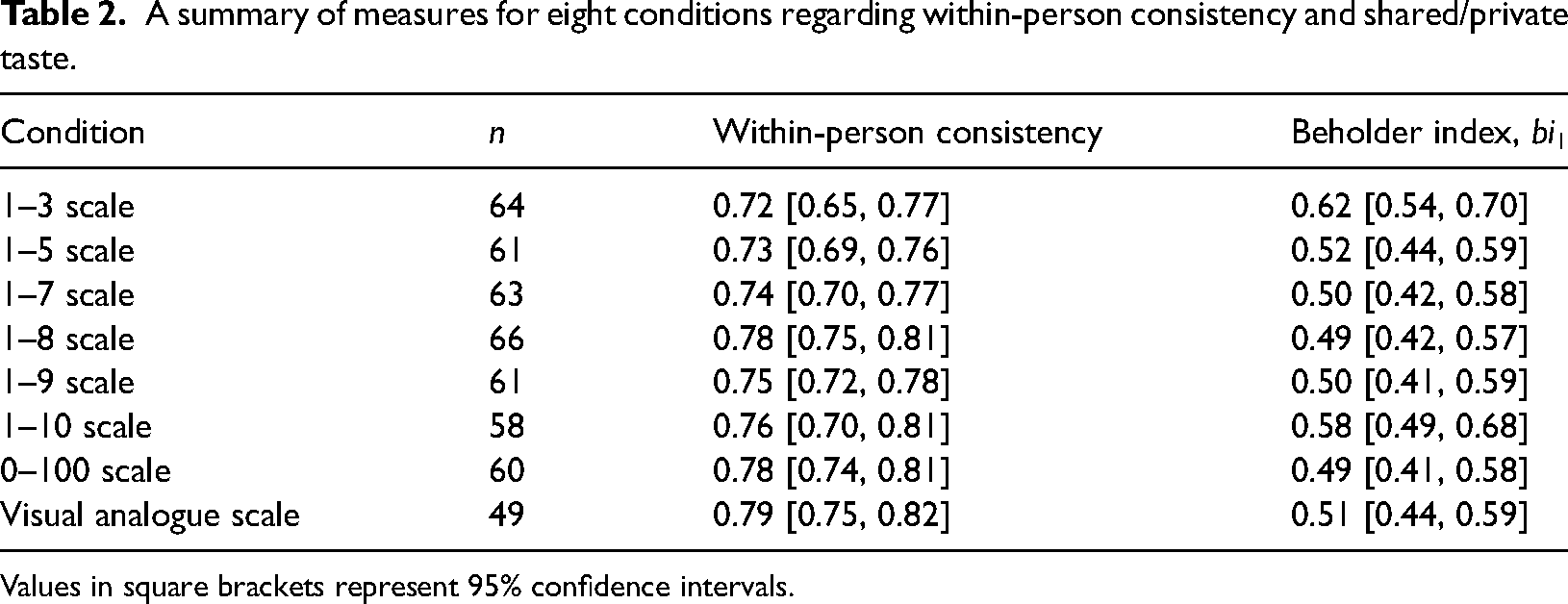
Values in square brackets represent 95% confidence intervals.

With the goal of quantifying the contributions of shared versus private taste, Hönekopp (2006) proposed a measure which represented the proportion of meaningful variance stable across time that arises from private taste – the beholder index, bi. By asking participants to rate the set of faces twice, one can differentiate between the observed variance attributed to participants, stimuli, time and their interactions. Here, we calculated bi₁ (the version of this index where absolute rater-score differences are assumed to be meaningless), with higher values representing greater contributions of private taste, and found that values were generally similar across scales, although somewhat higher for the 1–3 and 1–10 scales (see Table 2). A value of 0.50 represents equal contributions of shared and private taste, which was typically shown here.

Decomposing Variability Using Multilevel Models

Another way to consider how rating scales may differ in terms of their use is to decompose the variability in attractiveness ratings using multilevel models (following Hehman et al., 2017). This approach utilises the fact that multiple ratings were made by each participant and multiple ratings were given to each face. Since participants rated each face twice, a cross-classified model can estimate four sources of variability: (1) perceiver ICC – representing consistent differences between participants; (2) target ICC – accounting for consensually agreed-upon elements of attractiveness; (3) interaction ICC – quantifying personal/private taste; and (4) residual – measuring within-person consistency.

We used hierarchical Bayesian models to estimate these variance components. For each rating scale separately, these models fit a grand intercept parameter, a residual standard deviation (i.e., error), and the standard deviations of three normal distributions with means of zero that the individual random effects were drawn from, for participants, faces, and the interaction between the two, respectively. By squaring these four standard deviations (the residual and three random effects), we obtained the total variance, and the contribution of each source was then obtained by dividing the variance estimate by the total. Note that, despite using Bayesian inference, we simply took the mean of the posterior distribution of these values to aid clarity, as well as comparison with previous work.

The results of this analysis are shown in Figure 1. Overall, we found that the response scales were relatively similar in terms of their decomposition. However, our results suggest that private taste (interaction ICC) perhaps played a smaller role for the 1–7 and 1–9 scales, and a larger role for the 1–3 scale (with this latter result aligning with the bi₁ findings above). Inspection of the residual indicates that within-person consistency was lower (i.e., producing a larger residual) for scales with fewer response options (aligning with the pattern suggested in Table 2). Finally, we note that there were greater differences between participants (perceiver ICC) when using the 1–9 and 1–10 scales, which perhaps represents a disadvantage of using these particular scales.

Figure 1.

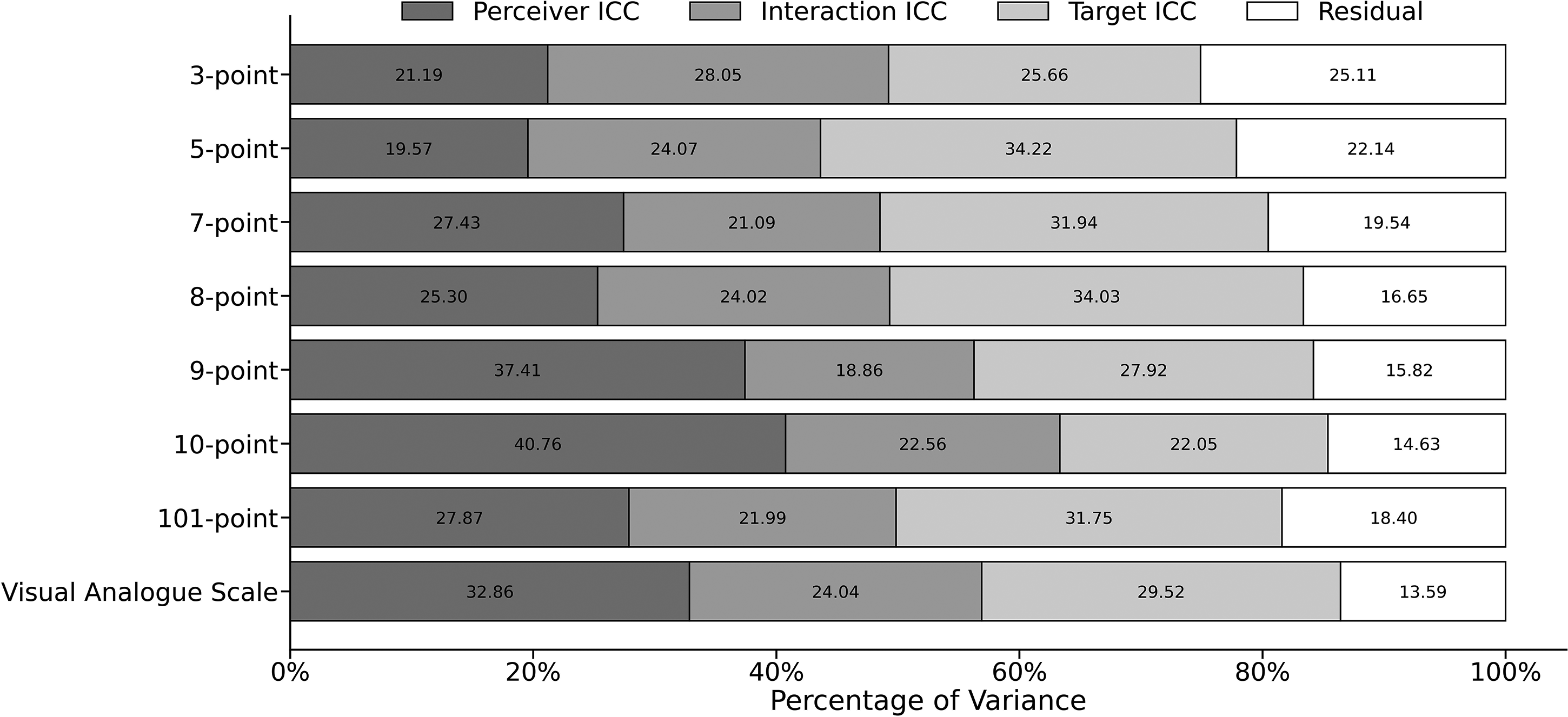
Relative contributions of between participant (perceiver ICC), between face (target ICC), between participant×face combinations (interaction ICC), and the residual, separately for each response scale.

Binary Response

Fifty-three participants completed the binary scale condition, where responses were limited to two response options: ‘unattractive’ or ‘attractive’. Typical measures of inter-rater agreement and within-person consistency could not be calculated here, given the binary nature of the data. As such, to quantify inter-rater agreement, we calculated a version of the average inter-rater agreement described above. However, rather than calculating the correlation between every possible pair of raters, we calculated the proportion of responses that were the same for these pairs. The average proportion was 0.66, 95% CI [0.65, 0.66], denoting that 66% of responses were identical for a given pair of raters (on average).

In order to quantify within-person consistency, we calculated the proportion of responses that were the same when comparing each rater's first and second blocks. The average proportion across all raters was 0.89, 95% CI [0.87, 0.91]. In other words, on average, participants repeated 89% of their responses across the two blocks.

Scale Use and Simple Equating

As a final step, we explored the frequency of scale use across each scale, simply by calculating the frequency of responses across both faces and raters. These frequencies are shown in Figure 2. To check if scale use was relatively consistent between scales, we estimated a simple linear association between each scale and the VAS, as the VAS is an unconstrained, continuous measure with no feedback on the response values. We averaged the responses in each scale for each face, and then carried out a series of regressions, predicting VAS scores from each scale separately. The slope from each regression indicates the amount of change in a scale that leads to a one-unit increase in the VAS. We used Bayesian estimation (with flat priors on the predictor) and recovered the posterior of the predictor. These are shown in Figure 3. If responses are used consistently between rating scales, a straightforward hypothesis is that the continuous response was simply divided between the available categories. For example, the 101-point scale mapped to the 1–3 point scale would mean that faces scoring below approximately 33 on the VAS would be given a 1, between 33 and 66 a 2, and so on. Regressing the 1–3 scale onto the VAS would then yield the amount that the VAS changes with a one-unit change in the 1–3 scale. As can be seen in Figure 3, the 1–5, 1–7, 1–8 and 101-point scale posterior estimates captured this naïve equating hypothesis – the equal division point was within the posterior estimate. However, the binary, 1–3, 1–9 and 1–10 scales showed an upward bias, such that the coefficient was greater than the simple division point.

Figure 2.

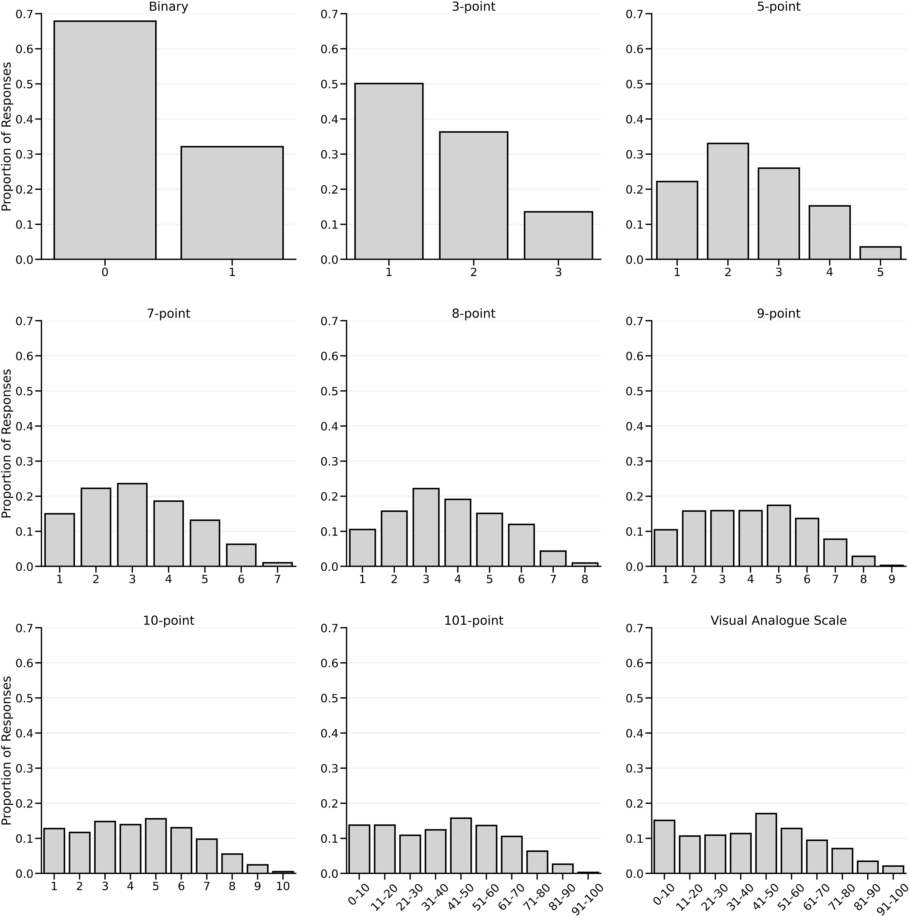
Histograms displaying the proportion of responses for each response option for each scale. The 101-point and VAS scales are binned within decile ranges for clarity.

Figure 3.

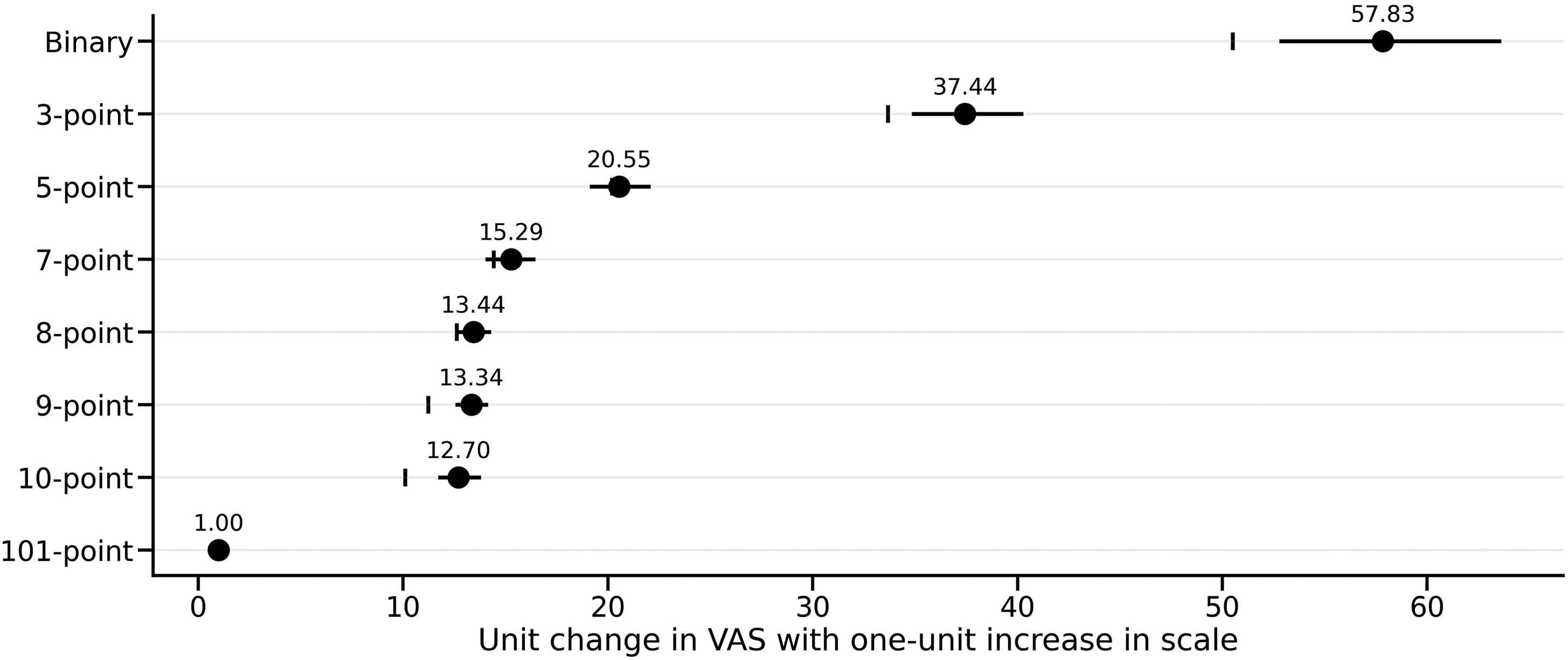
The coefficient and 95% credible interval resulting from a regression of each scale on to the VAS, with the vertical lines indicating the simple division of the VAS range into the number of responses available for the scale in question.

Discussion

In this study, we explored a range of questions relating to the psychometric properties of commonly used response scales for attractiveness perception. Our results provided little evidence of differences between the response scales investigated. As Tables 1 and 2 illustrate, considering measures of both inter-rater agreement and within-person consistency, values were similar across the scales. Perhaps the only noticeable result was that the 1–3 scale appeared to demonstrate lower inter-rater agreement, and correspondingly higher private taste, than the other scales. In addition, response scales with fewer options seemed to result in lower within-person consistency (see Figure 1 and Table 2). As such, we might recommend that small numbers of response options should be avoided if inter-rater agreement and within-person consistency are important for a particular study's outcomes.

Our regression analyses (see Figure 3) also provided evidence that the binary, 1–3, 1–9 and 1–10 scales did not seem to equate to a simple division of the VAS responses. That is, for these four response types, participant usage did not correspond to the division of the VAS into equally-sized categories (e.g., ten categories of approximately ten units each for the equivalent of the 1–10 scale). Therefore, researchers might avoid these response types in favour of using the 1–5, 1–7 and 1–8 scales since their use was more indicative of equally-sized, and perhaps more interpretable, scale units.

This recommendation, perhaps simply by chance, aligns with the literature in this field since the 1–7 scale in particular has been widely used over the years (e.g., Ma, Correll, et al., 2015; Penton-Voak et al., 2001; Rhodes et al., 2005; Sutherland et al., 2013). However, reassuringly, we found no substantial evidence for researchers to avoid any of the response scales investigated here. Until now, the common practice for measuring perceptions of facial attractiveness has been to select a scale based simply on researcher intuitions – for instance, does a 5-point scale feel sufficiently sensitive for the question being considered? While our findings suggest small benefits in the use of certain response scales, our overall conclusion is that, for the most part, the importance of choosing one scale over another is only minimal.

Given that the current measures of inter-rater agreement were also calculated in previous work for attractiveness ratings of unfamiliar faces (Kramer et al., 2018), we might consider these values side-by-side for our 1–7 scale (the length of scale used in their work). These were as follows (ours/theirs): Cronbach's α: 0.98/0.93; ICC(A,k): 0.97/0.91; average ‘leave one out’: 0.70/0.76; Kendall's W: 0.43/0.63; average inter-rater agreement: 0.49/0.61. For the two versions of intraclass correlation coefficient, our values were higher, but as mentioned earlier, this may simply have been due to our larger sample size. For the remaining three measures, we obtained lower values of agreement. Kramer et al. (2018) presented unfamiliar celebrity images that were obtained through Google's image search and were therefore unconstrained in appearance with regard to facial expression, background, clothing, lighting, etc. In contrast, our Chicago face database images featured identities posing front-on, wearing the same t-shirt, displaying neutral expressions, in front of the same background, and with the same camera set-up. Therefore, it is likely that the lower inter-rater agreement found here was the result of our using a more homogeneous set of stimuli, which resulted in a larger contribution of private taste (Hönekopp, 2006).

Indeed, we can also directly compare our measures of within-person consistency and shared/private taste with those obtained by Kramer et al. (2018), again for the 1–7 scale. These were as follows (ours/theirs): within-person consistency: 0.74/0.78; bi₁: 0.50/0.31. As suggested above, we found a substantially greater contribution of private taste in our data, most likely due to the use of a more homogeneous set of stimuli.

Finally, our values for decomposing variability can also be compared with those obtained by Hehman et al. (2017) (Analysis 3), who used a 1–7 scale and presented findings relating to a combined ‘youthful/attractiveness’ dimension. These were as follows (ours/theirs): perceiver ICC: 0.27/0.13; interaction ICC: 0.21/0.34; target ICC: 0.32/0.32; residual: 0.20/0.21. Interestingly, both sets of data were obtained using images of men and women taken from the Chicago face database (Ma, Correll, et al., 2015), and so it is unclear as to why we found larger differences between participants (perceiver ICC) and a smaller role of private taste (interaction ICC). This may be the result of those researchers combining youthfulness ratings with perceptions of attractiveness, or that we selected our stimuli to evenly span the full range of attractiveness values (based on available norming data). As such, larger differences between faces would be expected to result in private taste featuring less prominently (Hönekopp, 2006).

In general, across our different response scales, we found that private taste explained approximately half of the variance in attractiveness judgements. Although likely to be somewhat dependent on the specific set of face images featured, this finding is in broad agreement with previous work investigating facial attractiveness (e.g., Hönekopp, 2006; Kramer et al., 2018; Leder et al., 2016a, 2016b). In contrast, other types of stimuli have shown a substantially larger influence of private (in comparison with shared) taste on preference judgements (abstract artworks – Leder et al., 2016a, 2016b; architecture – Vessel et al., 2018), perhaps because these categories were artefacts of human culture rather than naturally occurring domains (Vessel et al., 2018). Further work will likely consider additional stimulus categories when tackling this question, and our findings suggest that the method of collecting participants’ preferences will have little influence on outcomes.

In the current work, we focussed on the perception of facial attractiveness since this is perhaps the most common trait investigated by researchers. However, there are several other traits that have played an influential role in face perception research (e.g., dominance and trustworthiness – Oosterhof & Todorov, 2008) and it would be interesting to consider whether response methods differed in their psychometric properties for such traits. Although we have no reason to believe that participants use the various response scales differently across different traits, this remains an empirical question for future studies to answer.

To conclude, we have provided a comprehensive investigation of the psychometric attributes associated with methods of measuring perceived facial attractiveness. For decades, studies have utilised response scales where participants have explicitly rated face images. However, none have considered the properties associated with these scales. Our study is the first to do so, and has demonstrated that scale choice (we imagine many researchers will be pleased to learn) will likely have little effect on experimental outcomes.

Footnotes

Acknowledgements

The authors thank our Research Skills III students for collecting the data, and Abi Davis for her input during the project's conceptualisation.

Author Contribution(s)

Robin Kramer: Conceptualization; Data curation; Formal analysis; Investigation; Methodology; Project administration; Visualization; Writing – original draft; Writing – review & editing.

Kay L. Ritchie: Conceptualization; Investigation; Methodology; Writing – review & editing.

Tessa R. Flack: Conceptualization; Investigation; Methodology; Writing – review & editing.

Michael O. Mireku: Investigation; Writing – review & editing.

Alex L. Jones: Formal analysis; Visualization; Writing – original draft.

Declaration of Conflicting Interests

The authors declared no potential conflicts of interest with respect to the research, authorship, and/or publication of this article.

Funding

The authors received no financial support for the research, authorship, and/or publication of this article.

ORCID iDs

Robin Kramer

Kay L. Ritchie

Tessa R. Flack

References

Alwin

D. F.

(1997). Feeling thermometers versus 7-point scales: Which are better? Sociological Methods & Research, 25, 318–340. https://doi.org/10.1177/0049124197025003003

Anwyl-Irvine

A. L.

Massonnié

Flitton

Kirkham

Evershed

J. K.

(2020). Gorilla in our midst: An online behavioral experiment builder. Behavior Research Methods, 52, 388–407. https://doi.org/10.3758/s13428-019-01237-x

Ballew

C. C.,

II Todorov

(2007). Predicting political elections from rapid and unreflective face judgments. Proceedings of the National Academy of Sciences, 104, 17948–17953. https://doi.org/10.1073/pnas.0705435104

Baumgartner

Steenkamp

J.-B. E. M.

(2001). Response styles in marketing research: A cross-national investigation. Journal of Marketing Research, 38, 143–156. https://doi.org/10.1509/jmkr.38.2.143.18840

Benson

P. L.

Karabenick

S. A.

Lerner

R. M.

(1976). Pretty pleases: The effects of physical attractiveness, race, and sex on receiving help. Journal of Experimental Social Psychology, 12, 409–415. https://doi.org/10.1016/0022-1031(76)90073-1

Bronstad

P. M.

Russell

(2007). Beauty is in the “we” of the beholder: Greater agreement on facial attractiveness among close relations. Perception, 36, 1674–1681. https://doi.org/10.1068/p5793

Burton

Fisher

Peña

P. G.

Rhodes

Ewing

(2021). Beyond Likert ratings: Improving the robustness of developmental research measurement using best–worst scaling. Behavior Research Methods, 53, 2273–2279. https://doi.org/10.3758/s13428-021-01566-w

Burton

Rigby

Sutherland

C. A.

Rhodes

(2019). Best-worst scaling improves measurement of first impressions. Cognitive Research: Principles and Implications, 4, 36. https://doi.org/10.1186/s41235-019-0183-2

Chen

(2015). What is the optimal number of response alternatives for rating scales? From an information processing perspective. Journal of Marketing Analytics, 3, 69–78. https://doi.org/10.1057/jma.2015.4

10.

Colman

A. M.

Norris

C. E.

Preston

C. C.

(1997). Comparing rating scales of different lengths: Equivalence of scores from 5-point and 7-point scales. Psychological Reports, 80, 355–362. https://doi.org/10.2466/pr0.1997.80.2.355

11.

Cooper

P. A.

Geldart

S. S.

Mondloch

C. J.

Maurer

(2006). Developmental changes in perceptions of attractiveness: A role of experience? Developmental Science, 9, 530–543. https://doi.org/10.1111/j.1467-7687.2006.00520.x

12.

Cortina

J. M.

(1993). What is coefficient alpha? An examination of theory and applications. Journal of Applied Psychology, 78, 98–104. https://doi.org/10.1037/0021-9010.78.1.98

13.

Cox

E. P.,

III . (1980). The optimal number of response alternatives for a scale: A review. Journal of Marketing Research, 17, 407–422. https://doi.org/10.1177/002224378001700401

14.

Cronbach

L. J.

(1951). Coefficient alpha and the internal structure of tests. Psychometrika, 16, 297–334. https://doi.org/10.1007/BF02310555

15.

Dion

K. L.

Berscheid

Walster

(1972). What is beautiful is good. Journal of Personality and Social Psychology, 24, 285–290. https://doi.org/10.1037/h0033731

16.

Donnachie

Jones

Jahoda

(2021). Facial attraction: An exploratory study of the judgements made by people with intellectual disabilities. Journal of Intellectual Disability Research, 65, 452–463. https://doi.org/10.1111/jir.12823

17.

Dourado

G. B.

Volpato

G. H.

de Almeida-Pedrin

R. R.

Oltramari

P. V. P.

Fernandes

T. M. F.

Conti

A. C. D. C. F.

(2021). Likert Scale vs visual analog scale for assessing facial pleasantness. American Journal of Orthodontics and Dentofacial Orthopedics, 160, 844–852. https://doi.org/10.1016/j.ajodo.2020.05.024

18.

Faust

N. T.

Chatterjee

Christopoulos

G. I.

(2019). Beauty in the eyes and the hand of the beholder: Eye and hand movements’ differential responses to facial attractiveness. Journal of Experimental Social Psychology, 85, 103884. https://doi.org/10.1016/j.jesp.2019.103884

19.

Germine

Russell

Bronstad

P. M.

Blokland

G. A. M.

Smoller

J. W.

Kwok

Anthony

S. E.

Nakayama

Rhodes

Wilmer

J. B.

(2015). Individual aesthetic preferences for faces are shaped mostly by environments, not genes. Current Biology, 25, 2684–2689. https://doi.org/10.1016/j.cub.2015.08.048

20.

Hauser

D. J.

Schwarz

(2016). Attentive Turkers: MTurk participants perform better on online attention checks than do subject pool participants. Behavior Research Methods, 48, 400–407. https://doi.org/10.3758/s13428-015-0578-z

21.

Hehman

Sutherland

C. A.

Flake

J. K.

Slepian

M. L.

(2017). The unique contributions of perceiver and target characteristics in person perception. Journal of Personality and Social Psychology, 113, 513–529. https://doi.org/10.1037/pspa0000090

22.

Hofmans

Theuns

(2008). On the linearity of predefined and self-anchoring Visual Analogue Scales. British Journal of Mathematical and Statistical Psychology, 61, 401–413. https://doi.org/10.1348/000711007X206817

23.

Hönekopp

(2006). Once more: Is beauty in the eye of the beholder? Relative contributions of private and shared taste to judgments of facial attractiveness. Journal of Experimental Psychology: Human Perception and Performance, 32, 199–209. https://doi.org/10.1037/0096-1523.32.2.199

24.

Jacoby

Matell

M. S.

(1971). Three-point Likert scales are good enough. Journal of Marketing Research, 8, 495–500. https://doi.org/10.1177/002224377100800414

25.

Kampe

K. K. W.

Frith

C. D.

Dolan

R. J.

Frith

(2001). Reward value of attractiveness and gaze. Nature, 413, 589–589. https://doi.org/10.1038/35098149

26.

Kendall

(1948). Rank correlation methods. Charles Griffin & Co.

27.

Kendall

M. G.

Smith

B. B.

(1939). The problem of m rankings. The Annals of Mathematical Statistics, 10, 275–287. https://doi.org/10.1214/aoms/1177732186

28.

Kramer

R. S. S.

Jones

A. L.

(2022). Incomplete faces are completed using a more average face. Cognitive Research: Principles and Implications, 7, 79. https://doi.org/10.1186/s41235-022-00429-y

29.

Kramer

R. S. S.

Jones

A. L.

Sharma

(2013). Sequential effects in judgements of attractiveness: The influences of face race and sex. PLoS ONE, 8, e82226. https://doi.org/10.1371/journal.pone.0082226

30.

Kramer

R. S. S.

Mileva

Ritchie

K. L.

(2018). Inter-rater agreement in trait judgements from faces. PLoS ONE, 13, e0202655.

31.

Kramer

R. S. S.

Mulgrew

Anderson

N. C.

Vasilyev

Kingstone

Reynolds

M. G.

Ward

(2020). Physically attractive faces attract us physically. Cognition, 198, 104193. https://doi.org/10.1016/j.cognition.2020.104193

32.

Kramer

R. S. S.

Pustelnik

L. R.

(2021). Sequential effects in facial attractiveness judgments: Separating perceptual and response biases. Visual Cognition, 29, 679–688. https://doi.org/10.1080/13506285.2021.1995558

33.

Lange

Kopkow

Lützner

Günther

K.-P.

Gravius

Scharf

H.-P.

Stöve

Wagner

Schmitt

(2020). Comparison of different rating scales for the use in Delphi studies: Different scales lead to different consensus and show different test-retest reliability. BMC Medical Research Methodology, 20, 28. https://doi.org/10.1186/s12874-020-0912-8

34.

Langlois

J. H.

Roggman

L. A.

(1990). Attractive faces are only average. Psychological Science, 1, 115–121. https://doi.org/10.1111/j.1467-9280.1990.tb00079.x

35.

Leder

Goller

Rigotti

Forster

(2016a). Private and shared taste in art and face appreciation. Frontiers in Human Neuroscience, 10, 155. https://doi.org/10.3389/fnhum.2016.00155

36.

Leder

Mitrovic

Goller

(2016b). How beauty determines gaze! Facial attractiveness and gaze duration in images of real world scenes. i-Perception, 7, 2041669516664355. https://doi.org/10.1177/2041669516664355

37.

Lehmann

D. R.

Hulbert

(1972). Are three-point scales always good enough? Journal of Marketing Research, 9, 444–446. https://doi.org/10.1177/002224377200900416

38.

Leung

S.-O.

(2011). A comparison of psychometric properties and normality in 4-, 5-, 6-, and 11-point Likert scales. Journal of Social Service Research, 37, 412–421. https://doi.org/10.1080/01488376.2011.580697

39.

Liao

H. I.

Kashino

Shimojo

(2021). Attractiveness in the eyes: A possibility of positive loop between transient pupil constriction and facial attraction. Journal of Cognitive Neuroscience, 33, 315–340. https://doi.org/10.1162/jocn_a_01649

40.

López Bóo

Rossi

M. A.

Urzúa

S. S.

(2013). The labor market return to an attractive face: Evidence from a field experiment. Economics Letters, 118, 170–172. https://doi.org/10.1016/j.econlet.2012.10.016

41.

Lozano

L. M.

García-Cueto

Muñiz

(2008). Effect of the number of response categories on the reliability and validity of rating scales. Methodology, 4, 73–79. https://doi.org/10.1027/1614-2241.4.2.73

42.

D. S.

Correll

Wittenbrink

(2015). The Chicago face database: A free stimulus set of faces and norming data. Behavior Research Methods, 47, 1122–1135. https://doi.org/10.3758/s13428-014-0532-5

43.

Luo

(2015). Children’s and adults’ judgments of facial trustworthiness: The relationship to facial attractiveness. Perceptual and Motor Skills, 121, 179–198. https://doi.org/10.2466/27.22.PMS.121c10x1

44.

McDonald

P. R.

Slater

A. M.

Longmore

C. A.

(2008). Covert detection of attractiveness among the neurologically intact: Evidence from skin-conductance responses. Perception, 37, 1054–1060. https://doi.org/10.1068/p5774

45.

Olson

I. R.

Marshuetz

(2005). Facial attractiveness is appraised in a glance. Emotion, 5, 498–502. https://doi.org/10.1037/1528-3542.5.4.498

46.

Oosterhof

N. N.

Todorov

(2008). The functional basis of face evaluation. Proceedings of the National Academy of Sciences, 105, 11087–11092. https://doi.org/10.1073/pnas.0805664105

47.

Orghian

Hidalgo

C. A.

(2020). Humans judge faces in incomplete photographs as physically more attractive. Scientific Reports, 10, 1–12. https://doi.org/10.1038/s41598-019-56437-4

48.

Pegors

T. K.

Mattar

M. G.

Bryan

P. B.

Epstein

R. A.

(2015). Simultaneous perceptual and response biases on sequential face attractiveness judgments. Journal of Experimental Psychology: General, 144, 664–673. https://doi.org/10.1037/xge0000069

49.

Penton-Voak

I. S.

Jones

B. C.

Little

A. C.

Baker

Tiddeman

Burt

D. M.

Perrett

D. I.

(2001). Symmetry, sexual dimorphism in facial proportions and male facial attractiveness. Proceedings of the Royal Society of London. Series B: Biological Sciences, 268, 1617–1623. https://doi.org/10.1098/rspb.2001.1703

50.

Pfeifer

(2012). Physical attractiveness, employment and earnings. Applied Economics Letters, 19, 505–510. https://doi.org/10.1080/13504851.2011.587758

51.

Preston

C. C.

Colman

A. M.

(2000). Optimal number of response categories in rating scales: Reliability, validity, discriminating power, and respondent preferences. Acta Psychologica, 104, 1–15. https://doi.org/10.1016/S0001-6918(99)00050-5

52.

Rezlescu

Penton

Walsh

Tsujimura

Scott

S. K.

Banissy

M. J.

(2015). Dominant voices and attractive faces: The contribution of visual and auditory information to integrated person impressions. Journal of Nonverbal Behavior, 39, 355–370. https://doi.org/10.1007/s10919-015-0214-8

53.

Rhodes

Simmons

L. W.

Peters

(2005). Attractiveness and sexual behavior: Does attractiveness enhance mating success? Evolution and Human Behavior, 26, 186–201. https://doi.org/10.1016/j.evolhumbehav.2004.08.014

54.

Ritchie

K. L.

Palermo

Rhodes

(2017). Forming impressions of facial attractiveness is mandatory. Scientific Reports, 7, 469. https://doi.org/10.1038/s41598-017-00526-9

55.

Rosenthal

(2018). Meta-analytic procedures for social research (2nd ed.). Sage.

56.

Simms

L. J.

Zelazny

Williams

T. F.

Bernstein

(2019). Does the number of response options matter? Psychometric perspectives using personality questionnaire data. Psychological Assessment, 31, 557–566. https://doi.org/10.1037/pas0000648

57.

Skrinda

Krama

Kecko

Moore

F. R.

Kaasik

Meija

Lietuvietis

Rantala

M. J.

Krams

(2014). Body height, immunity, facial and vocal attractiveness in young men. Naturwissenschaften, 101, 1017–1025. https://doi.org/10.1007/s00114-014-1241-8

58.

Sui

Liu

C. H.

(2009). Can beauty be ignored? Effects of facial attractiveness on covert attention. Psychonomic Bulletin & Review, 16, 276–281. https://doi.org/10.3758/PBR.16.2.276

59.

Sutherland

C. A.

Oldmeadow

J. A.

Santos

I. M.

Towler

Burt

D. M.

Young

A. W.

(2013). Social inferences from faces: Ambient images generate a three-dimensional model. Cognition, 127, 105–118. https://doi.org/10.1016/j.cognition.2012.12.001

60.

Taubert

Van der Burg

Alais

(2016). Love at second sight: Sequential dependence of facial attractiveness in an on-line dating paradigm. Scientific Reports, 6, 22740. https://doi.org/10.1038/srep22740

61.

Ueno

Ito

Kawasaki

Kawachi

Yoshida

Murakami

Sakai

Iijima

Matsue

Fujii

(2014). Neural activity associated with enhanced facial attractiveness by cosmetics use. Neuroscience Letters, 566, 142–146. https://doi.org/10.1016/j.neulet.2014.02.047

62.

Vessel

E. A.

Maurer

Denker

A. H.

Starr

G. G.

(2018). Stronger shared taste for natural aesthetic domains than for artifacts of human culture. Cognition, 179, 121–131. https://doi.org/10.1016/j.cognition.2018.06.009

63.

Weijters

Cabooter

Schillewaert

(2010). The effect of rating scale format on response styles: The number of response categories and response category labels. International Journal of Research in Marketing, 27, 236–247. https://doi.org/10.1016/j.ijresmar.2010.02.004

64.

White

Burton

A. L.

Kemp

R. I.

(2016). Not looking yourself: The cost of self-selecting photographs for identity verification. British Journal of Psychology, 107, 359–373. https://doi.org/10.1111/bjop.12141

65.

Willis

Todorov

(2006). First impressions: Making up your mind after a 100-ms exposure to a face. Psychological Science, 17, 592–598. https://doi.org/10.1111/j.1467-9280.2006.01750.x

66.

Wilson

J. P.

Rule

N. O.

(2015). Facial trustworthiness predicts extreme criminal-sentencing outcomes. Psychological Science, 26, 1325–1331. https://doi.org/10.1177/0956797615590992

67.

Winston

J. S.

O’Doherty

Kilner

J. M.

Perrett

D. I.

Dolan

R. J.

(2007). Brain systems for assessing facial attractiveness. Neuropsychologia, 45, 195–206. https://doi.org/10.1016/j.neuropsychologia.2006.05.009

68.

Zebrowitz

L. A.

Franklin

R. G.,

Jr. Hillman

Boc

(2013). Older and younger adults’ first impressions from faces: Similar in agreement but different in positivity. Psychology and Aging, 28, 202–212. https://doi.org/10.1037/a0030927

The psychometrics of rating facial attractiveness using different response scales

Abstract

Keywords

Method

Participants

Stimuli

Procedure

Results

Inter-Rater Agreement

Within-Person Consistency and Shared/Private Taste

Decomposing Variability Using Multilevel Models

Binary Response

Scale Use and Simple Equating

Discussion

Footnotes

Acknowledgements

Author Contribution(s)

Declaration of Conflicting Interests

Funding

ORCID iDs

References