
Abstract
The time it takes for a stimulus to reach awareness is often assessed by measuring reaction times (RTs) or by a temporal order judgement (TOJ) task in which perceived timing is compared against a reference stimulus. Dissociations of RT and TOJ have been reported earlier in which increases in stimulus intensity such as luminance intensity results in a decrease of RT, whereas perceived perceptual latency in a TOJ task is affected to a lesser degree. Here, we report that a simple manipulation of stimulus size has stronger effects on perceptual latency measured by TOJ than on motor latency measured by RT tasks. When participants were asked to respond to the appearance of a simple stimulus such as a luminance blob, the perceptual latency measured against a standard reference stimulus was up to 40 ms longer for a larger stimulus. In other words, the smaller stimulus was perceived to occur earlier than the larger one. RT on the other hand was hardly affected by size. The TOJ results were further replicated in a simultaneity judgement task, suggesting that the effects of size are not due to TOJ-specific response biases but more likely reflect an effect on perceived timing.
Introduction
How long does it take for a visual stimulus to reach visual awareness? The difficulty in answering this question lies in the observation that neural processing time of visual events can be dissociated from subjective experience of the timing of those visual events (Dennett & Kinsbourne, 1992; Nishida & Johnston, 2002, and, for a more general discussion about the relation between neural processing and conscious experience, see Overgaard & Mogensen, 2014). For example, Nishida and Johnston (2002) showed that differences in processing latency cannot account for situations in which simultaneous events are perceived to occur at different times. In addition, answering this question is complicated by the fact that at least two types of methods can be dissociated that assess whether a stimulus is needed for action or perception (for an overview, see e.g., Cardoso-Leite & Gorea, 2010). The first type of method is argued to reflect the time for a stimulus to trigger a motor response, while the second type reflects the time for subjective perception to emerge. For example, simple reaction times (SRTs; responding as fast as possible to a stimulus whose onset time varies) would classify as reflecting motor latency, 1 whereas temporal order judgements (TOJ) would classify as reflecting perceptual latency.
Several studies have investigated the effects of variations in stimulus parameters on these two types of measures (motor and perceptual). Increases in the intensity of auditory stimuli (Sanford, 1971, 1974) and in the luminance intensity of visual stimuli (Cattell, 1886; Exner, 1868; Pins & Bonnet, 1996; Roufs, 1963, 1974) generally lead to decreases in SRT. This is known as Piéron’s law in psychophysics (Piéron, 1952). The dependency of reaction times (RTs) on stimulus intensity has been explained in terms of an accumulation of sensory evidence of a stimulus being present (Gold & Shadlen, 2001; Link, 1992; Link & Bonnett, 1998; Luce, 1986; Smith & Ratcliff, 2004). In such models, sensory evidence for the presence of a stimulus increases faster when the stimulus intensity is high, thus allowing for a faster response.
Many studies using both SRT and TOJ report that effects of variations in stimulus intensity have a bigger effect on SRT than on TOJ (for an exception, see Roufs, 1963 and for a metareview, see Cardoso-Leite & Gorea, 2010). For example, larger effects of stimulus intensities on RTs compared with TOJs have been reported for spatial frequency (Barr, 1983; Gish, Shulman, Sheehy, & Leibowitz, 1986; Tappe, Niepel, & Neurmann, 1994), retinal position (Jaskowski, 1987), stimulus duration (Jaskowski, 1992), attention (Neumann, Esselmann, & Klotz, 1993), salience (Adams & Mamassian, 2004), and the presence of a preceding stimulus (Kanai, Carlson, Verstraten, & Walsh, 2009).
Attempts have been made to account for the differential effects of stimulus intensity on SRTs and TOJs within a single framework (Cardoso-Leite, Gorea, & Mamassian, 2007; Ejima & Ohtani, 1987; Gibbon & Rutschmann, 1969; Jaskowski, 1993; Miller & Schwarz, 2006; Sternberg & Knoll, 1973). These attempts are in part based on observations that effects of stimulus parameters on SRT and TOJ are correlated when both methods are combined into a single design (Cardoso-Leite et al., 2007). Those attempts suggest that the temporal dissociations of TOJs and SRTs can be explained by distinct decision criteria or by different time markers for the two types of decisions even if common signal sources were assumed for both cases. Another account of the temporal dissociation is a dual-route hypothesis in which motor response and perception for a stimulus are thought to take different processing paths (Neumann, 1990; Neumann et al., 1993; Tappe et al., 1994).
In the present study, we report a novel temporal dissociation for TOJs and RTs in which the two methods are dissociated by changes in stimulus size. We examined how stimulus size affects perceived timing in TOJ, simultaneity judgment, choice RT, and SRT tasks. Previous studies have shown that SRTs are shorter for larger stimuli (Harwerth & Levi, 1978; Marzi, Mancini, Metitieri, & Savazzi 2006; Osaka, 1976; Sperandio, Savazzi, Gregory, & Marzi, 2009). However, effects of stimulus size on TOJ tasks have not been established. Crucially, our experiments reveal that the effects of stimulus size on perceived timing in TOJ tasks are dissociated from the effects on RT tasks: Smaller stimuli are perceived to occur earlier than larger ones, while effects of size on RTs are absent or in the other direction (in which RT decreases with increasing size).
Experiment 1
Methods
Apparatus
Stimuli were presented using the Psychtoolbox on a 22′ LaCie III CRT (running at 100 Hz, with a resolution of 1024 × 768 pixels) via a Mac Pro (Apple Inc., CA).
Participants
Ten naïve observers (all undergraduates at the Psychology department of Utrecht University) with normal or corrected-to-normal vision performed in all experiments. The head of the observer was supported by a chinrest, which stood at a distance of 57 cm to the screen. This study was conducted in accordance with the Declaration of Helsinki.
Stimuli and procedures
In Experiment 1, participants were tested on a TOJ task and a speeded choice reaction time (CRT) task. In the TOJ task, observers were asked to indicate which of two Gaussian blobs, presented left and right of fixation, appeared first. Stimuli were presented at 12° eccentricity (centre to fixation cross). One of the two blobs (the standard stimulus) always had a sigma of 1°, while the other (the test stimulus) had a sigma of 0.5°, 1°, or 3°. The blobs had a peak luminance of 69.2 cd m−2. Background luminance of the screen was 35.5 cd m−2. Weber contrast of the peak luminance of the blob with the background was 94.9%.
To estimate the point of subjective simultaneity (PSS) for each stimulus size, we used a method of constant stimuli in which stimulus onset asynchrony (SOA) between the standard and the test stimulus was varied between −300 ms, −100 ms, −50 ms, −20 ms, 0 ms, +20 ms, +50 ms, +100 ms, and +300 ms. Here, positive SOAs correspond to the conditions in which the standard was presented before the test stimulus. Both stimuli remained on the screen until 500 ms had passed since the appearance of the first stimulus (see top row of Figure 1). Each participant completed 20 trials per condition. Differently sized stimuli and different SOAs were presented in random order. In addition, the fixed-sized stimulus could be presented left or right of fixation, which also occurred in random order. The experiment was performed in a self-paced manner whereby participants initiated a trial by pressing the space bar. At that time, a green fixation cross appeared which was followed by the stimulus with an onset varying randomly between 500 and 1000 ms later. To obtain the PSS, we fitted the fraction standard stimulus first responses for different SOAs to a cumulative normal distribution function with parameters µ (mean) and σ (standard deviation). In the context of this experiment, the µ parameter corresponds to the PSS (see Figure 2 for the fitted data). Participants were instructed to fixate on the fixation cross throughout the experiment and to refrain from making eye movements. In the TOJ task, observers were instructed to indicate which of two Gaussian blobs occurred earlier, the one on the left (by using the left arrow key) or the one on the right (by using the right arrow key).
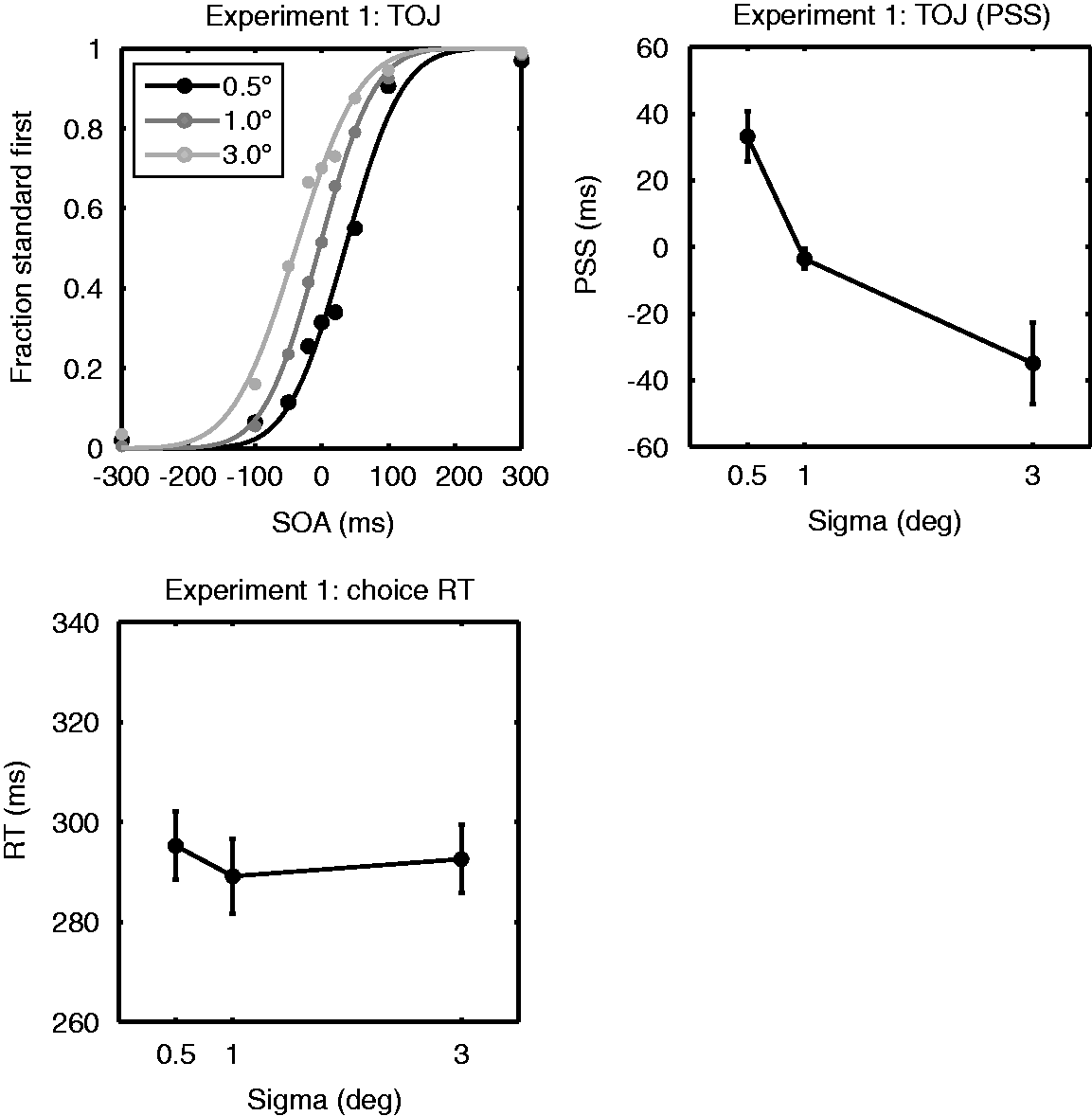
Schematic representation of the sequence of events during single trials. The top row represents a possible order of events in the TOJ experiment. The middle row represents events in TOJ experiments (Experiments 1 and 2), the bottom row events for RT experiments (Experiments 1–3). In TOJ experiments, the instruction was to report (not speeded) at what side of fixation one of two Gaussian blobs (Experiment 1) or one of two Gabors (Experiment 2) appeared first. In CRT experiments (Experiments 1 and 2), the instruction was to respond as fast and accurately as possible the location (left or right of fixation) of the stimulus. In the SRT experiment (Experiment 3), the instruction was to respond as fast and accurately to the appearance of a Gaussian blob or Gabor. Results of Experiment 1. The top row represents the results for the TOJ experiment. The top left panel shows the TOJ data fitted to a cumulative normal function. The data-points represent the average fraction “standard first” responses for the 10 observers; the lines represent the fits for these average fractions. Black, dark gray, and light gray lines and circles represent, respectively, the data for the conditions where the test stimulus was smaller, of equal size or larger than the standard stimulus. The top right panel shows the PSS taken from the fitted cumulative normal functions. The bottom row shows choice reaction times for Gaussian blobs of different sizes. Error bars represent SEM. CRT was not modulated by stimulus size.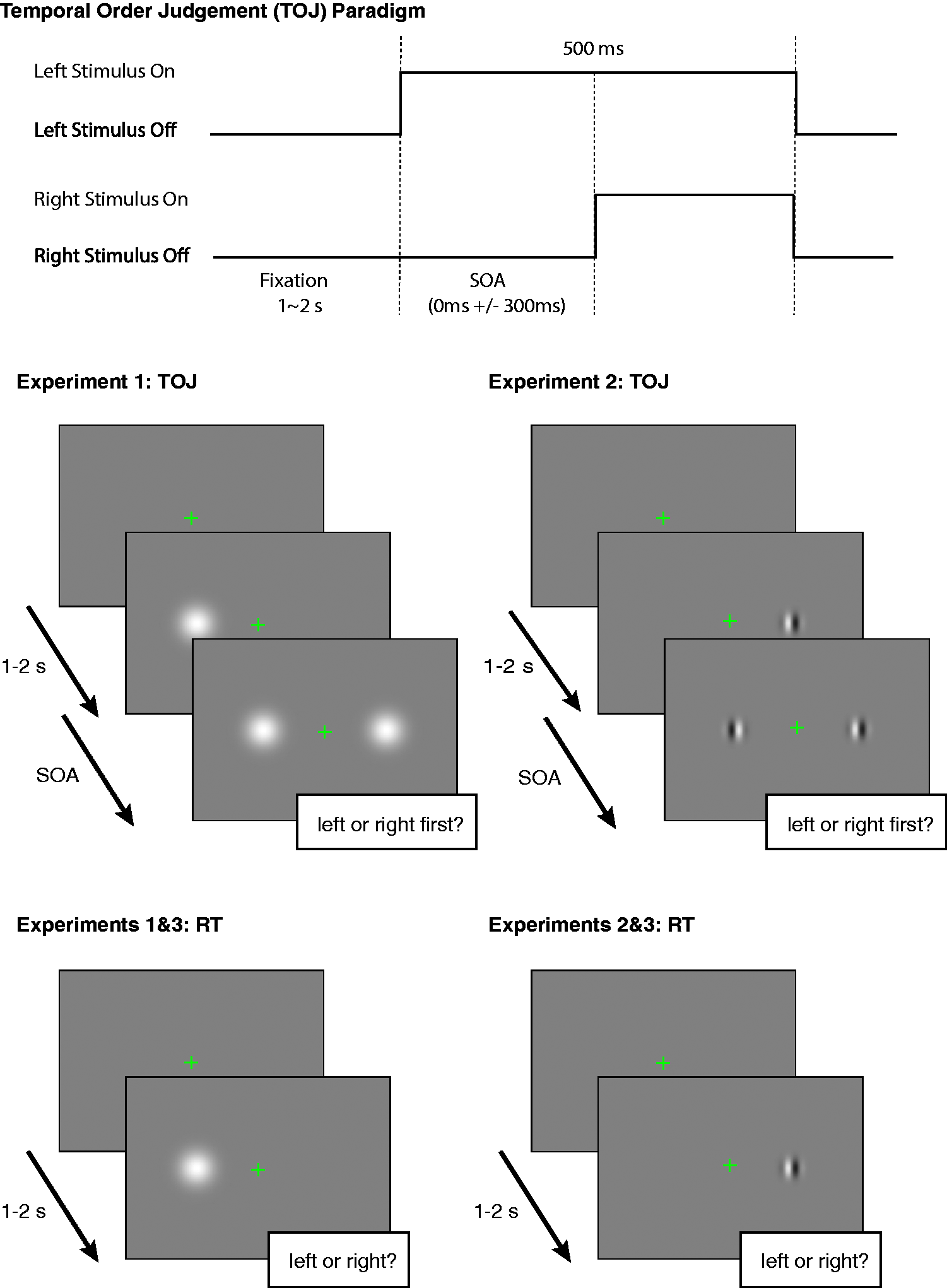
In the CRT task, the size parameter σ of the Gaussian blobs was also varied across 0.5°, 1°, or 3° of visual angle. The blob was presented at 12° eccentricity, either left or right of a centrally presented fixation cross. The stimulus remained on the screen until the participant responded. RTs were measured for 20 trials per condition (10 trials per each side). The order of trials (i.e., different sizes and side of presentation) was fully randomised. For the RT task too, participants were instructed to fixate on the fixation cross throughout the experiment and to refrain from making eye movements. In the RT task, observers were instructed to indicate as fast and accurately as possible whether the Gaussian blob occurred on the left (by using the left arrow key) or the right (by using the right arrow key) side of fixation.
To assure comparison of the RT results with the TOJ experiment, stimulus parameters such as background luminance, eccentricity, and peak luminance of the Gaussian blobs were kept identical for the two tasks. For the RT experiment, only correct trials (left or right) were included in the analysis. The participants showed nearly perfect accuracy: The lowest accuracy among participants was 96.3%, and the mean accuracy was 98.8%. Observers started with the RT task, followed by the TOJ task. The TOJ task was performed in five blocks; the RT task in one block.
Analysis
A one-way repeated measures analysis of variance (ANOVA) was performed to determine whether size influenced RT or PSS in the two experiments. For all RT experiments (including Experiments 2 and 3), RTs 2.5 standard deviations below or above the mean were removed. Bonferroni correction was applied for post hoc pairwise significance tests when the ANOVA revealed a significant main effect.
Results and Discussion
The results of the TOJ experiment show that changes in stimulus size had a significant effect on the PSS. The PSS for sizes 0.5°, 1.0°, and 3.0° were 33(8), 2 −4 (3), and −35 (12) ms, respectively. A repeated measures ANOVA revealed a main effect of size of the Gaussian blobs (Figure 2, top right: F(2, 18) = 13.0, p < .004). 3 More specifically, PSSs were significantly different for sizes 0.5° and 1.0° (p = .004), and for 0.5° and 3° (p = .013), but not for size 1.0° and 3.0° (p = .095). Importantly, the PSS for the 0.5° blob was significantly larger than zero, t(9) = 4.6, p = .001, and that of the 3° blob was significantly smaller than zero, t(9) = 3.0, p = .008. These results reveal that the test blob was perceived earlier when it was smaller than the standard blob, whereas it was perceived later when it was larger. The PSS for the 1° blob was not significantly different from zero, t(9) = 1.3, p = .2, indicating that two blobs of equal size were judged to appear at about the same time.
In the CRT experiment, changes in stimulus size did not influence the RT at least within the range tested in our study (Figure 2, bottom left). Mean RTs were 295(7), 289(8), and 293(7) ms for 0.5°, 1.0°, and 3.0° blobs, respectively. A repeated measures ANOVA for average RTs for the RT task revealed that RTs were not significantly different for different sizes of the blobs, F(2, 18) = 0.50, p = .62.
While the TOJ experiment reveals that larger stimuli are perceived later than smaller stimuli, we did not find a strong dependency of CRT on stimulus size. This seems to contradict previous findings that RT decreases as the size of simple visual stimuli becomes larger (Marzi et al., 2006; Osaka, 1976; Sperandio et al., 2009). This discrepancy may come from the fact that we employed a CRT task in which participants had to make a judgement about the position (i.e., left or right) of the target, whereas the previous studies used a SRT as the measure of objective processing speed. Although the CRT task in our study was very simple, it required a decision about stimulus position, and this may have eliminated the size dependency effect shown for SRTs (Marzi et al., 2006; Osaka, 1976; Sperandio et al., 2009). We address the difference between CRT and SRT tasks in Experiment 3, in which we used a SRT task with the same set of stimuli.
Taken together, CRTs do not decrease with increasing stimulus size, as would be in line with what we observed for the TOJ task.
Experiment 2
In Experiment 1, we assumed that perceived timing was modulated by stimulus size. However, it is conceivable that differences in spatial frequency components led to differences in perceived timing. For example, the power spectrum of the spatial frequency components of a Gaussian blob spread to higher frequencies when the σ of the Gaussian is small. Given the differential sensitivity of the magno and parvo pathways to different spatial frequencies (Livingstone & Hubel, 1988; Kulikowski & Tolhurst, 1973), one may hypothesise that spatial frequency rather than stimulus size determines perceived timing.
The purpose of Experiment 2 was to determine whether perceptual delay for a large stimulus is caused by differential processing of spatial frequency or by the spatial extent of the stimulus. To this end, we varied the spatial frequency and spatial extent of a Gabor stimulus independently and examined their impact on perceived timing. For comparison, CRTs were measured for the same set of Gabor stimuli used in the TOJ experiment.
Methods
Apparatus
The setup used in Experiment 2 was identical to that used in Experiment 1.
Participants
The same 10 observers as in Experiment 1 took part in this experiment. The head of the observer was supported by a chinrest, which stood at a distance of 57 cm to the screen. The observers were instructed to fixate on the fixation cross and to refrain from making eye movements during the trials. This study was conducted in accordance with the Declaration of Helsinki.
Stimuli and procedures
In Experiment 2, we conducted a TOJ task and a CRT task using Gabor stimuli (see Figure 1). Participants were again asked to indicate which of two Gabor stimuli, presented left and right of fixation at 12° eccentricity (centre to fixation cross), were presented first. One of the Gabors (the standard) always had a sigma of 1° and a spatial frequency of 0.5 cycles per degree (cpd), while the spatial frequency and sigma of the other Gabor (the test) were varied across 0.25, 0.5, or 2 cpd, and 0.5°, 1.0°, or 3.0°, respectively. The phases of the Gabor stimuli were fixed; all phases were aligned such that a transition from black to white was positioned at the centre of the stimulus. The peak luminance contrast of Gabors was always set to 94.4% Michelson. As in Experiment 1, SOA (standard minus test) was varied across −300 ms, −100 ms, −50 ms, −20 ms, 0 ms, +20 ms, +50 ms, +100 ms, and +300 ms. Both stimuli stayed on the screen until 500 ms had passed since the appearance of the first stimulus. The fraction of reporting the standard stimulus to have appeared first was estimated based upon 20 trials per condition. Differently sized stimuli, different spatial frequencies, and different SOAs were presented in random order. In addition, the fixed-sized stimulus could be presented left or right of fixation, which also occurred in random order. As in Experiment 1, the experiment progressed in a self-paced manner. The PSS for each condition was again estimated by fitting a cumulative normal distribution function to the data (see Figure 3 for the fitted data).
Results of Experiment 2. The top row shows the TOJ data fitted to a cumulative normal function (from left to right: data for 0.25, 0.5, and 2.0 cpd Gabors). The data-points represent the average fraction “standard first” responses for the 10 observers; the lines represent the fits for these average fractions. Black, dark gray, and light gray lines and circles represent, respectively, the data for the conditions where the test stimulus was smaller, of equal size or larger than the standard stimulus. The bottom left panel shows the PSS taken from the fitted cumulative normal functions: solid lines and squares for 0.25 cpd Gabors, dashed lines and triangles for 0.5 cpd Gabors, and dotted lines and diamonds for the 2.0 cpd Gabors. The bottom right panel shows choice reaction times for Gaussian blobs of different size and spatial frequency. Again, solid lines and squares show RTs for 0.25 cpd Gabors, dashed lines and triangles for 0.5 cpd Gabors, and dotted lines and diamonds for the 2.0 cpd Gabors.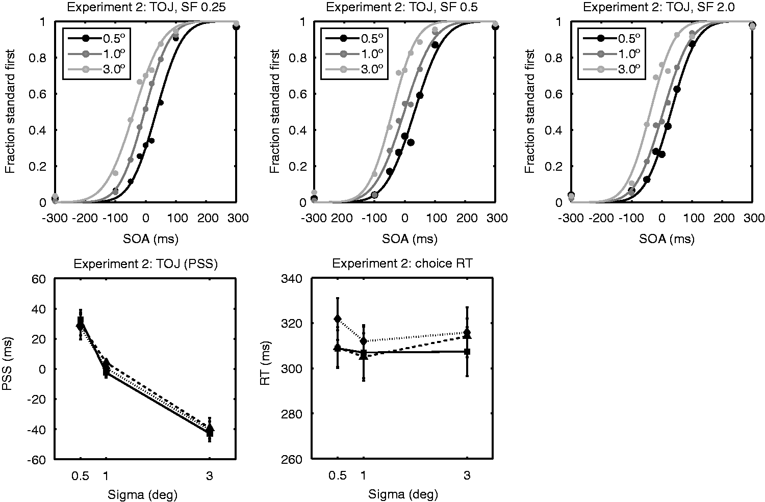
For comparison, a CRT task was conducted for the same set of Gabor stimuli (spatial frequency: 0.25, 0.5, or 2 cpd; sigma: 0.5°, 1.0°, or 3.0°). In this task, participants were required to indicate whether a single Gabor stimulus was presented to the left or to the right. The stimulus was presented either left or right of a central fixation cross, at 12° eccentricity. Again, the stimulus remained on the screen until the participant responded. RT was computed for each of the nine conditions by averaging the RTs for 20 trials per condition. Order of presentation was randomised, and incorrect trials were excluded from the analysis. Observers again started with the RT task, followed by the TOJ task. The TOJ task was performed in 10 blocks, the RT task in 2 blocks.
Analysis
Both for the TOJ and RT experiments, a two-way repeated measures ANOVA was performed on the PSS data from the TOJ task or the mean RT data from the CRT task. With this analysis, we tested main effects of stimulus size and spatial frequency, and the interaction between these two factors. Bonferroni correction was applied for post hoc pairwise significance tests when the ANOVA revealed a significant main effect.
Results and Discussion
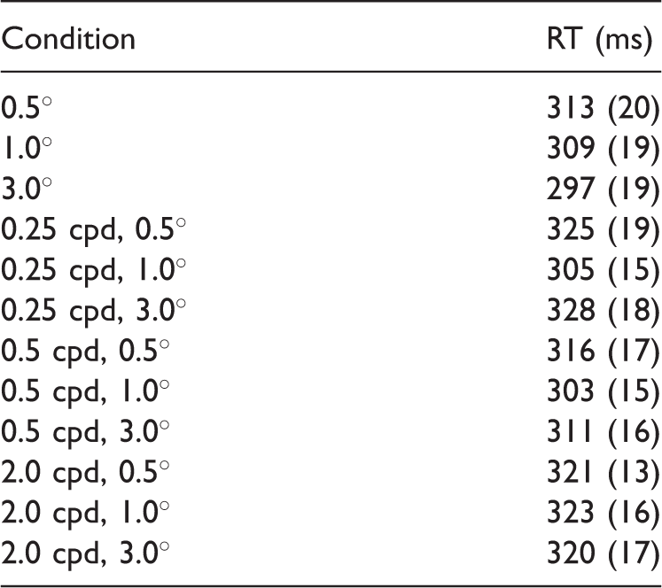
Point of Subjective Simultaneity and Reaction Time in ms for Each Size and Spatial Frequency.
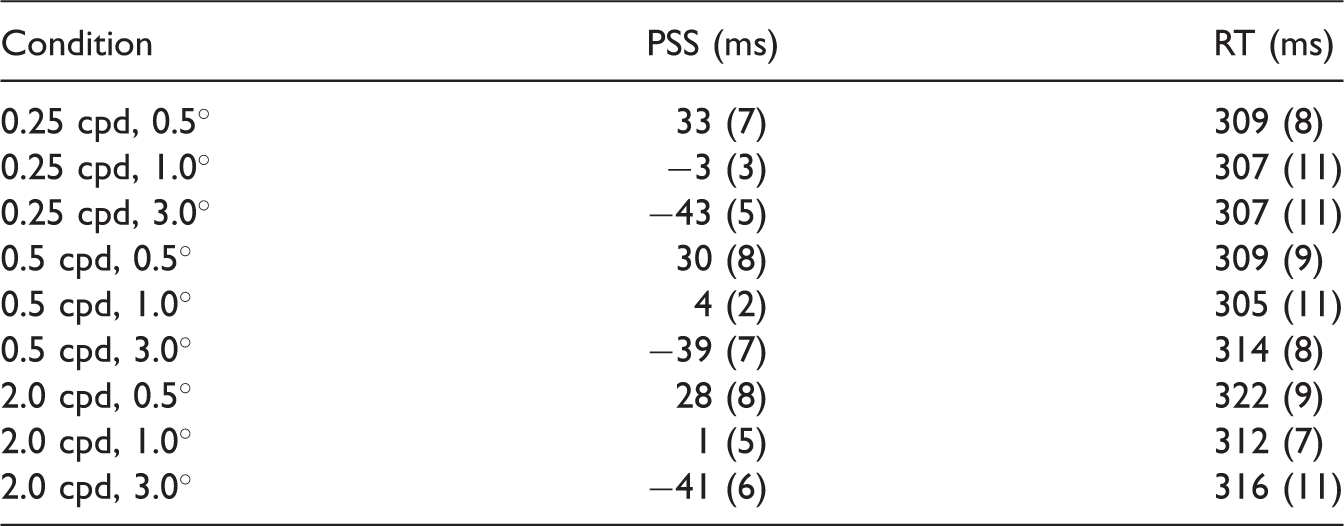
Note. cpd = cycles per degree; PSS = point of subjective simultaneity; RT = reaction time.
Values between brackets represent standard errors of the mean.
The CRT results obtained for the same set of Gabor stimuli showed different patterns than the TOJ results (Figure 3, bottom right and Table 1). A repeated measures ANOVA revealed no main effect of size, F(2, 18) = 2.22, p = .14, a main effect of spatial frequency, F(2, 18) = 10.8, p = .001, and no significant interaction between them (p = .53). Post hoc comparisons revealed that RTs of sizes 0.5° and 1.0° were significantly different (p = .043, two-sided, Bonferroni corrected), but there was no significant difference in the RT for 1.0° versus 3.0° Gabors, and for 0.5° versus 3.0° Gabors (p > .62, two-sided, Bonferroni corrected). 4 These results together indicate a tendency that CRTs for Gabors get smaller for larger stimuli (CRTs were shorter for 1.0° Gabors compared with 0.5° Gabors). This trend is opposite to what was observed for PSS. For spatial frequency, the mean RTs collapsed across stimulus size showed significant difference between the 0.25 and 2.0 cpd conditions (p = .005, Bonferroni corrected) and the 0.5 and 2.0 cpd conditions ( = .04, Bonferroni corrected) indicating that the 2.0 frequency stimuli were responded slower to than lower frequency stimuli (mean RT 0.25 cpd = 308 ms, mean RT 0.5 cpd = 309 ms, and mean RT 2 cpd = 317 ms).
The TOJ task in Experiment 2 indicates that perceptual delay for large stimuli is driven by the spatial extent of a stimulus rather than its spatial frequency contents, suggesting that the spatial extent covered by a stimulus is the fundamental factor in determining the timing of conscious perception. Furthermore, the dissociation of PSS from RTs in the effect of stimulus size was again demonstrated for the same set of stimuli in Experiment 2. Spatial frequency had an effect on CRTs, whereas no effect was observed for PSS.
While our results of the TOJ experiment suggest that the size effect is driven by spatial extent rather than spatial frequency, this interpretation needs to be treated with caution. The size of the sigma of the Gabor envelopes was relatively small (0.5°, 1°, or 3°) compared with the spatial frequencies used in the current experiment. For this reason, the carrier frequency should not be taken nominally, and further exploration is needed to establish the lack of effects of spatial frequency on TOJ. However, the lack of spatial frequency effects on TOJ has also been previously reported using higher spatial frequencies (2cpd–8 cpd with 1° wide stimuli; Tappe et al., 1994) and may hold for a broader range of conditions. Taken together, effects of spatial frequency on TOJ seem minimal, and further experiments would be needed to further establish this result for a greater range of combinations of spatial extent and spatial frequency.
Our result that CRT increased with spatial frequency is consistent with previous studies. The relationship between spatial frequency and SRT has been extensively investigated in the past. The general finding is that RT increases with spatial frequency (Breitmeyer, 1975; Ejima & Ohtani, 1987; Gish et al., 1986; Harwerth & Levi, 1978; Ludwig, Gilchrist, & McSorley, 2004; Lupp, Hauske, & Wolf, 1976; Musselwhite & Jeffreys, 1985; Tappe et al., 1994; Tartaglione, Goff, & Benton, 1975; Vassilev & Mitov, 1976).
Experiment 3
The results of Experiments 1 and 2 show that CRTs decrease slightly with increasing stimulus size. However, effects of stimulus size on RT have mainly been investigated using SRT tasks (Osaka, 1976; Harwerth & Levi, 1978; Marzi et al. 2006, Sperandio et al., 2009), while we used CRT tasks. In Experiment 3, we used the same stimuli as in Experiments 1&2, but now with applying a SRT task.
Methods
Participants
Ten new observers took part in this experiment (all undergraduates at the psychology department of Utrecht University). The head of each observer was supported by a chinrest, which stood at a distance of 57 cm to the screen. The observers were instructed to fixate on the fixation cross and to refrain from making eye movements during the trials. This study too was conducted in accordance with the Declaration of Helsinki.
Stimuli and Procedures
In Experiment 3, we conducted a SRT task using Gaussian blobs and Gabor stimuli. On every trial, a green fixation cross would appear. Between 1000 and 2000 ms, later (the timing was randomly varied) the stimulus would appear left or right of fixation. Participants were asked to press a button (the spacebar) as fast and accurately as possible when a stimulus, presented left and right of fixation at 12° eccentricity (centre to fixation cross), appeared. Sizes of Gaussian blobs were equal to those of Experiment 1; sizes and spatial frequencies of Gabors were equal to those of Experiment 2. Importantly, the setup used for Experiment 3 was identical to Experiments 1 and 2, ensuring that stimuli were identical in all three Experiments. Each observer performed three blocks: two for Gabor stimuli and one for Gaussian blobs. Within each block, different stimuli (blobs of different sizes and Gabors of different size and spatial frequency) were presented in random order. The three blocks were run in random order. Again, participants completed 20 trials per condition. As in Experiments 1 and 2, the stimulus remained on the screen until the participant responded. Incorrect trials were excluded from the analysis.
Results and Discussion
The results of Experiment 3 are presented in Figure 4 and Table 2. A repeated measures ANOVA revealed no significant main effect for size of the Gaussian blobs, F(2, 18) = 2.94, p = .08. This result indicates that there is a trend for SRT to decrease with increasing stimulus size. A repeated measures ANOVA for the Gabors revealed significant main effects for both size and spatial frequency, respectively, F(2, 18) = 3.9, p = .04; F(2, 18) = 5.42, p = .014, but no significant interaction, F(4, 36) = 1.61, p = .19. Post hoc testing revealed that SRTs were not significantly different between different sizes (after Bonferroni correction for multiple comparisons: p > .08). The latter trend-level significance refers to the trend for SRTs to be shorter for 1.0° Gabors compared with 0.5° Gabors. Post hoc testing for the effect of spatial frequency revealed that the difference between Gabors of 0.5 and 2.0 cpd was significant (p = .014). The latter indicates that SRTs to 2.0 cpd Gabors were longer than to 0.5 cpd Gabors.
Results of Experiment 3. The left panel shows simple reaction times for Gaussian blobs of different sizes; the right panel for Gabors of different size and spatial frequency. Again, solid lines and squares show RTs for 0.25 cpd Gabors, dashed lines and triangles for 0.5 cpd Gabors, and dotted lines and diamands for the 2.0 cpd Gabors. Reaction Time in ms for Blobs and Gabors, for Each Size and Spatial Frequency. Note. cpd = cycles per degree; RT = reaction time. Values between brackets represent standard errors of the mean.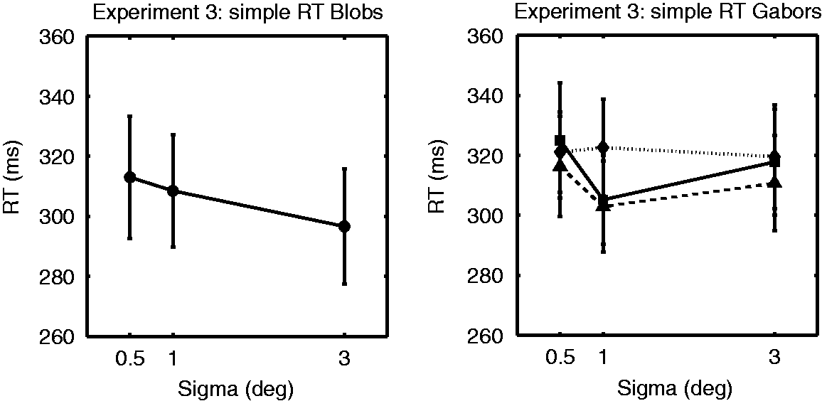
Experiment 4
In Experiments 1 to 3, stimulus size was manipulated by changing the dispersion of the Gaussian envelope defining the extent of the Gaussian blob. However this manipulation also alters the luminance distribution of the stimulus. Experiment 4 addressed this possible confound by running the TOJ task with black Gaussian blobs. If larger stimuli are still perceived as coming earlier then our effects cannot be explained in terms of size-modulated changes to the luminance distribution.
Methods
Apparatus
Stimuli were presented using Psychtoolbox on a 22′ Dell Trinitron CRT (running at 100 Hz, with a resolution of 1024 × 768 pixels) via a PC running Windows XP.
Participants
Data were collected from 13 naïve undergraduate and postgraduate students at the University of Sussex. Two observers’ data were excluded because their data did not follow a cumulative normal distribution. This left 11 participants for analysis. The experiment received ethical approval from the University of Sussex ethics committee.
Stimuli and Procedure
Experiment 4 was identical to the TOJ component of Experiment 1 except that the Gaussian blobs were black. Background luminance was 21.6 cd m−2, and minimum luminance of the Gaussian blob was 1.3 cd m−2 for this experiment. Weber contrast of the peak luminance of the blob with the background was 94.0%. As in Experiment 1, participants performed 20 trials per stimulus size and SOA.
Results and Discussion
Results from Experiment 4 replicated the significant effect of size on PSS, F(1.21, 12.11) = 6.40, p = .022 (Greenhouse-Geisser corrected). The PSS for sizes 0.5°, 1.0°, and 3.0° were 15(7), −5 (5), and −46 (17) ms, respectively. However, the difference between 0.5° and 1°, 1° and 3°, and 0.5° and 3° did not reach significance after Bonferroni-correction (p = .113, p = .025, and p = .025 uncorrected respectively). Results are shown in Figure 5. Importantly, the PSS for the 0.5°, stimulus was marginally greater than zero, t(10) = 1.99, p = .075, for the 1°, stimulus was not significantly different from zero, t(10) = −0.87, p = .407, and for the 3°, stimulus was significantly less than zero, t(10) = −2.69, p = .023. To compare the results of this experiment (using black blobs) with those of Experiment 1 (using white blobs), we performed a repeated measures ANOVA with size as within- and luminance as between-subject factor. This analysis revealed a main effect of size, F(2, 38) = 16.8, p < .0001, no significant main effect of luminance, F(1, 19) = 3.2, p = .09, and no significant interaction between both factors, F(2, 38) = 0.3, p = .74. This analysis again confirms our observation that stimulus size affected perceived timing of visual events. At first sight, the trending significance level of the between-subject factor luminance might give the impression that luminance had some influence on perceived timing. However, this effect merely indicates that PSEs for white blobs (Experiment 1) were (at a trending significance level) generally larger compared with PSEs for black blobs (this experiment). Importantly, the analysis reveals that luminance did not significantly interact with stimulus size: Perceived timing was not differentially affected by white compared with black blobs.
Results of Experiment 4. The left panel shows the TOJ responses averaged over participants as a function of size (from left to right, 0.5°, 1°, and 3°) and latency. The averaged behavioural data are indicated by circular markers. The fitted cumulative normal distributions are indicated by solid lines. The right panel shows the mean PSS for each stimulus size. Error bars represent +/−1 SEM.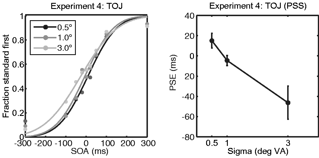
Experiment 5
Although the TOJ task suggests that larger stimuli are perceived as arriving earlier, the task cannot discriminate between perceptual or decisional effects of size. More specifically, observers could be biased toward reporting smaller stimuli as having arrived first without a perceptual effect on the PSS. This concern was addressed in Experiment 5 by running Experiment 1 as a simultaneity judgment (SJ) task. By fitting a Gaussian distribution to the proportion of same responses, we can distinguish between perceptual effects of size (which would manifest in changes to central tendency) and response effects (which would manifest in changes to the amplitude of the distribution).
Methods
Apparatus
The setup was identical to that in Experiment 4.
Participants
The same observers as in Experiment 4 took part in this experiment. One participant was excluded because the data did not follow a Gaussian distribution.
Stimuli and Procedure
Experiment 5 was identical to the TOJ component of Experiment 1, except that participants were asked whether the two blobs appeared at different times (right arrow key) or simultaneously (left arrow key). Stimuli were white Gaussian blobs. Participants performed 20 trials per stimulus size and SOA.
The order in which participants performed the Experiments 4 and 5 was fully counterbalanced.
Analysis
For each observer and stimulus size, we computed the proportion of simultaneous responses as a function of latency. These proportions were fit to a scaled Gaussian using the nonlinear least squares method, and the central tendency and amplitude parameters were subjected to separate repeated-measures ANOVAs.
Results and Discussion
Results are shown in Figure 6. A log transformation was applied to the amplitude data because obtained values are close to the upper bound of 1. A repeated measures ANOVA revealed a significant effect of size on amplitude, F(2, 18) = 5.53, p = .013. The amplitudes (corresponding to fraction simultaneous responses) were 0.81 (0.06), 0.92 (0.05), and 0.79 (0.07) for sizes 0.5°, 1.0°, and 3.0°, respectively. Specifically, there was a quadratic relationship, F(1, 9) = 7.94, p = .020, such that observers were more biased toward reporting simultaneous for equally sized than unequally sized stimuli. There was also a significant effect of size on central tendency, F(2, 18) = 9.63, p = .001. The PSS for sizes 0.5°, 1.0°, and 3.0° were 5 (4), 1 (1), and −13 (3) ms, respectively. Central tendency for the 3° stimulus took a significantly lower value than that of the 1° (−13 ms +/− 3 ms vs. 1 ms +/− 1 ms, p = .005) and 0.5° (−13 ms +/− 3 ms vs. 5 ms +/− 4 ms, p = .005) stimuli (Bonferroni corrected). There was no significant difference between the 0.5° and 1° stimuli (p > .999). Together, these results reveal that response effects (reflected by differences in amplitude) are involved in the effects of size on perceived timing, but that perceptual effects (revealed by differences in central tendency) are clearly involved. Importantly, the results support and extend those of Experiments 1, 2, and 4 by indicating that small stimuli are perceived as arriving before a larger standard.
Results of Experiment 5. The top left panel represents the SJ responses averaged over participants as a function of size (from left to right, 0.5°, 1°, and 3°) and latency. The averaged behavioural data are indicated by circular markers. The fitted cumulative normal distributions are indicated by solid lines. The top right panel depicts the mean central tendency of the Gaussian pdfs fitted to the simultaneity judgements, as a function of stimulus size. The bottom left panel depicts the mean amplitude of these distributions as a function of stimulus size. Error bars represent +/−1 SEM.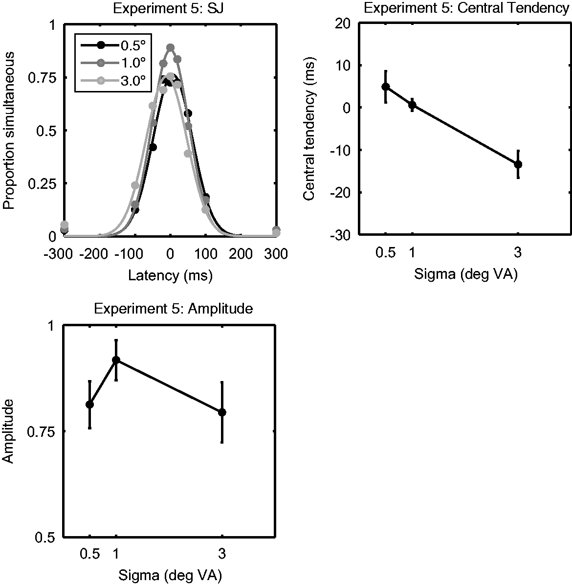
General Discussion
The main finding of the current study is that a small stimulus appears to occur earlier than a larger one both in a TOJ task and SJ task. This result contrasts with effects of stimulus size in CRT and SRT tasks. The effects of stimulus size on TOJ were not driven by differences in spatial frequency components but were determined by the spatial extent covered by the stimulus. Moreover, the changes in perceived timing were dissociated from the changes in CRTs (Experiments 1 and 2) and from changes in SRT (Experiment 3), which have been reported in the literature earlier (Harwerth & Levi, 1978; Marzi et al., 2006; Osaka, 1976; Sperandio et al., 2009). These results make a case for a temporal dissociation in which stimulus size has different effects in perceptual judgement (i.e., TOJ and SJ) tasks and speeded response (i.e., SRT and CRT) tasks. These findings are of interest in the light of the well-established principle that stimuli with greater intensity such as in luminance are responded to and perceived faster (Cattell, 1886; Exner, 1868; Piéron, 1952; Pins & Bonnet, 1996; Roufs, 1963, 1974).
The facilitation of RTs for larger stimuli can be explained by a simple race model. Suppose that reactive motor responses are triggered by the first set of spikes that reaches a certain threshold. The volley of spikes triggered independently over a greater retinotopic area would reach that stage probabilistically more quickly. One could also conceive a decision stage mechanism that pools inputs over space. In such a framework, a greater number of neurons triggered by a larger stimulus would produce a stronger signal as a collection and trigger a faster response. In these conceptualisations of RTs, faster responses observed for larger stimuli are not surprising, and indeed consistent with the known relationship between stimulus intensity and RTs.
On the other hand, the relationship between stimulus size and the timing of perception in the TOJ (and SJ) tasks requires an explanation. A first option would be that different mechanisms (a dual route) account for RT responses on the one hand TOJ responses on the other (e.g., Neumann, 1990; Neumann et al., 1993; Tappe et al., 1994). This option has been challenged by Cardoso-Leite et al. (2007) who showed that RT and TOJ are correlated when assessed in a single design. Another option, proposed by several authors, is a differential threshold model in which the thresholds are different for perception (TOJ) and for action (RT; Ejima & Ohtani, 1987; Jaskowski, 1993; Miller & Schwarz, 2006; Sternberg & Knoll, 1973). In such models, RT and TOJ responses are based on the same (neural) signal. The way to explain differences in effects on RT and TOJ is to assume different response criteria for both: Observers use a higher criterion for TOJ than for RT responses (Cardoso-Leite et al., 2007; Ejima & Ohtani, 1987; Miller & Schwarz, 2006; Sanford, 1974).
While the differential threshold model can capture the dissociation between perceptual and motor latencies, the model was proposed to explain the more widely observed tendency that RTs are more strongly affected by stimulus intensity or attentional manipulations compared with perceptual latency measured by TOJ (Barr, 1983; Cardoso-Leite et al., 2007; Jaskowski, 1992; Neumann et al., 1993; Roufs, 1963, 1974; Sanford, 1974; Steglich & Neumann, 2000; Tappe et al., 1994). Our results are opposite to this trend: Perceptual latency measured by TOJ or SJ tasks was more strongly affected by stimulus size than motor latency measured by RT tasks. Therefore, previous models with a lower threshold for TOJ compared with RT (Figure 7, left panel; e.g., Cardoso-Leite & Gorea, 2010) would predict results opposite to our findings. To account for our results within the same theoretical framework, the threshold for TOJ needs to be higher than for RTs. However, it is highly unlikely that decision criteria are reversed for RT and TOJ only when stimulus size is manipulated. To account for the discrepancy between our results and previous findings, a new model needs to be developed. One possible hypothesis is that the latency of the internal response has different offsets depending on the stimulus size in addition to the rate of signal accumulation (Figure 7, right panel). This model would explain the present results as well as the trend that RTs for larger stimuli were slightly shorter. This model remains highly speculative, and further evidence is warranted to support it.
Predictions of two models for dissociations between RT and TOJ. In both models, the internal signal to a stimulus linearly increases, and the slope of the increase is proportional to the strength of the stimulus (here, solid line for a high-intensity stimulus; dashed line for a low-intensity stimulus). Both models assume a higher internal criterion for an RT (c(RT)) compared with a TOJ (c(TOJ)) task. In the left panel, the latency of the start of the increase is equal for stimuli of different intensity. This model explains results where effects of stimulus intensity on RT are larger compared with effects on TOJ. In the right panel, the latency of the higher intensity stimulus (solid line) is higher than that of the lower intensity stimulus (dashed line). In the context of the present experiment, the lower intensity stimulus is a smaller stimulus; a higher intensity stimulus is a bigger stimulus. This model can explain the present results. It can potentially explain results why effects of stimulus intensity are bigger for RT compared with TOJ (by assuming a criterion for TOJ that is closer to that of the criterion for RT).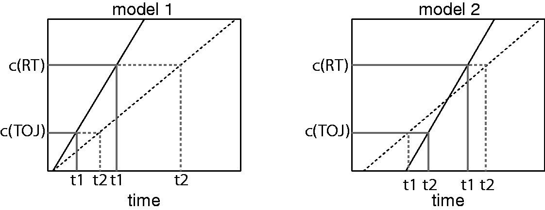
It can also be speculated that the results of the TOJ experiment are related to perceptual filling in. Filling in refers to the phenomenon that the colour and lightness from, for example, an annulus spread to the interior of the annulus (Komatsu, 2006; Lamme, Rodriquez-Rodriguez, & Spekreijse, 1999; Paradiso & Nakayama, 1991). It has been shown that perceptual filling is related to the built-up of activity in V1 of the macaque (Lamme et al., 1999). On a speculative note, the delayed perception of a large stimulus compared with a smaller one might come about by the fact that it might take more time to complete the representation of a larger stimulus (due to filling in of a larger stimulus area) compared with a smaller one. This built-up of activity would be irrelevant for the RT experiment: Any signal of the stimulus would suffice to start responding to the stimulus.
As an alternative explanation, one could argue that the delay of perceptual latency for larger stimuli may be mediated by a combination of two separate effects. First it has been known that large stimuli tend to be perceived to last longer (e.g., Ono & Kawahara, 2007; Rammsayer & Verner, 2015; Thomas & Cantor, 1975; Xuan, Zhang, He, & Chen, 2007). Therefore, it is logically possible that larger stimuli in our experiments were also perceived to last longer even though two stimuli were terminated simultaneously 500 ms after the onset of the first stimulus. Stimulus duration in turn could affect the timing of onset because of the known effect that the perceived onset of a stimulus is delayed for a longer lasting stimulus (e.g., Jaskowski, 1991; Kuling, van Eijk, Juola, & Kohlrausch, 2012). These combined effects could explain the size effect reported in the present study. Further research is warranted to determine whether perceived duration mediated the delay of perceived stimulus onset in our study.
In summary, we have demonstrated that small stimuli are perceived to appear earlier than bigger ones. This effect, observed in TOJ and SJ tasks, is dissociated from the processing time measured by SRT and CRTs. This RT–TOJ dissociation provides constraints on theories on the timing of perception. While stimulus size is a relatively simple feature of visual stimuli, simple manipulations in this dimension will provide a powerful experimental paradigm to further explore the neural correlates of time makers for subjective perceptual timing.
Footnotes
Acknowledgement
The authors would like to thank Sebastiaan Mathôt for his comments on the manuscript.
Declaration of Conflicting Interests
The author(s) declared no potential conflicts of interest with respect to the research, authorship, and/or publication of this article.
Funding
The author(s) disclosed receipt of the following financial support for the research, authorship and/or publication of this article: ESD was supported by was supported by the European Union FP7 Marie Curie ITN Grant N. 606901 (INDIREA).