
Abstract
National statistical agencies increasingly face budget constraints and shrinking sample sizes, while simultaneously gaining access to rich auxiliary data and powerful pre-trained machine learning (ML) and artificial intelligence (AI) models, including Large Language Models (LLMs). Traditional model-assisted estimation techniques, which fit models using survey sample data, are limited by small sample sizes, struggle to leverage complex non-linear relationships in auxiliary data, and cannot accommodate frontier pre-trained models. This work re-examines the use of pre-trained black-box models, fit independently of the survey sample, for design-based parameter estimation. Inspired by the Prediction-Powered Inference (PPI) framework, we introduce the Prediction-Powered Estimator (PPE), an unbiased estimator with an unbiased variance estimator for the survey design setting. We also formalize the use of pre-trained models with the classic difference estimator—which we term the Prediction-Powered Difference (PPD) estimator—and with the Generalized Regression Estimator via predicted values as covariates (
1. Introduction
Machine learning (ML) and artificial intelligence (AI) provide increasingly accurate prediction and imputation tools, with applications ranging from administrative data linkage to automated coding systems at national statistical agencies. At the same time, agencies have access to increasingly rich auxiliary data—administrative records, scanner data, images, and text. This convergence presents an opportunity to enhance survey estimation through pre-trained models fit on large external or historical datasets.
Our objectives are to (i) reduce sample sizes and respondent burden without sacrificing accuracy, (ii) accommodate useful non-linear, algorithmic models, including LLMs, and (iii) retain design-based unbiasedness of both estimators and variance estimators. Classical model-assisted methods such as the generalized regression (GREG) and model-calibrated (MC) estimators meet some, but not all, of these goals: they require fitting a (usually linear) model to the survey sample itself, risking overfitting as sample sizes shrink and precluding the use of large pre-trained black-box models.
A natural alternative is to rely on pre-trained models fitted on historical or external data. These models, independent of the current survey sample, can capture complex relationships unreachable with in-sample modeling. The chief concern is distribution shift between training and target populations. Motivated by the Prediction-Powered Inference (PPI) framework, we treat the pre-trained model as a black box and develop three complementary estimators: (1) the Prediction-Powered Estimator (PPE), a PPI-style design-based estimator with an unbiased variance formula; (2) the Prediction-Powered Difference (PPD) estimator, a difference estimator that uses model predictions; and (3)
Each approach offers distinct strengths. The difference estimator is simple and design-unbiased (Breidt and Opsomer 2017); PPE is unbiased and may gain efficiency through a negative covariance term;
The remainder of the paper is organized as follows: Section 2 reviews classical estimators and PPI. Section 3 extends PPI to the survey design setting, defining the PPE estimator and its variance estimator, and formalizes all three proposed estimation strategies. LLM-based use-cases are presented in Section 4, followed by experiments on real-world survey data from Statistics Canada in Section 5. Simulation experiments benchmarking the proposed estimators against classical baselines are provided in the Supplemental Material. Section 6 concludes.
2. Background
Survey methodologies aim to estimate population characteristics such as the total
2.1. Horvitz-Thompson Estimator
In the absence of auxiliary data, the Horvitz-Thompson (HT) estimator of the population mean is
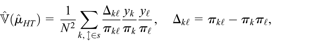
making it a reliable basis for design-based inference (Särndal et al. 1992, 43), though it does not exploit auxiliary information.
2.2. Model-Assisted Estimators
Assume a (row) vector of auxiliary variables
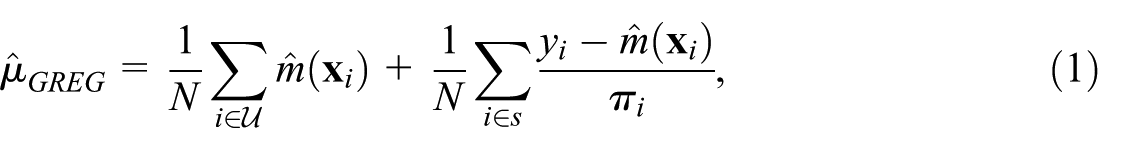
where
The Model-Calibrated (MC) estimator of Wu and Sitter (2001) extends GREG to non-linear models
2.3. Difference Estimator and Pre-Trained Models
For any values
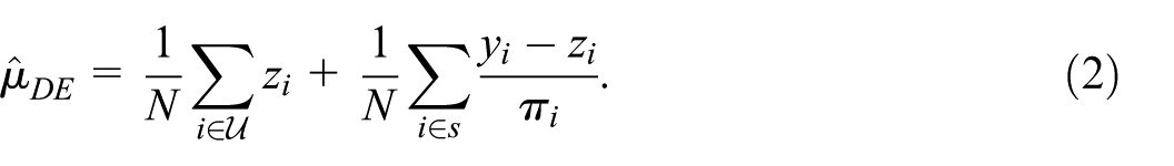
This estimator is design-unbiased, with unbiased variance estimator based on the residuals
When a pre-trained model
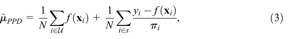
with unbiased variance estimator:
The variance decreases as model residuals shrink: a high-quality pre-trained model yields an efficient estimator. If there is significant distributional shift between training and survey data (concept drift), residuals may be large, reducing efficiency—but the estimator and variance estimator remain unbiased. The magnitude of concept drift can be assessed diagnostically from the survey sample residuals.
More precisely, the variance should be understood as a conditional variance, conditioned on the survey design, the pre-trained model
2.4. Recent Developments
Sanguiao-Sande and Zhang (2021) introduced a novel design-unbiased method known as subsampling Rao-Blackwellisation (SRB), which integrates modern machine learning (ML) techniques into the framework of design-based inference for finite populations. Their approach addresses the increasing use of complex, nonlinear ML models in survey sampling by maintaining design validity—ensuring inference remains grounded in the known sampling design, regardless of model correctness. The SRB method synthesizes three classical ideas in statistical inference: (i) model-assisted estimation, which uses auxiliary information to improve efficiency while preserving design-based properties; (ii) cross-validation, a standard technique in ML for estimating prediction error; and (iii) the Rao-Blackwell Theorem, which enhances estimator efficiency by conditioning on sufficient statistics. Unlike traditional model-assisted methods that rely on asymptotic design consistency, the SRB approach aligns with the Neyman-Fisher notion of consistency for finite populations, providing exact design-unbiasedness for a given population and sampling method while leveraging the predictive power of ML models. However, SRB requires fitting the model on subsets of the survey sample, limiting its applicability to complex or large model classes and making it computationally expensive.
Dagdoug et al. (2023) extended random forests to model-assisted estimation, showing asymptotic design-consistency. However, performance depends critically on the hyper-parameter
These approaches share a key limitation relative to the PPD/PPE framework: they fit models using the survey sample, which is typically small and shrinking. Pre-trained models, by contrast, are fit on large external datasets and treat the survey sample only as the labeled set for bias-correction.
2.5. Prediction-Powered Inference (PPI)
PPI was introduced by Angelopoulos et al. (2023a) and quickly gained attention within the ML research community, with extensions including Bayesian PPI (Hofer et al. 2024), CrossPPI (Zrnic and Candès 2024b), PPI++ (Angelopoulos et al. 2024), and a generalization to active statistical inference (Zrnic and Candès 2024a). Despite its promise, no prior work has adapted PPI to the survey design setting.
PPI assumes access to a black-box model
where
PPI, PPD, and model-assisted estimators such as GREG share similar mathematical forms but differ in two key respects relevant to the survey design setting. First, GREG fits a linear model on the survey sample, while PPI, PPD, and MC place no restriction on the model class. Second, and more importantly, the use of auxiliary data differs: for PPD, GREG, and MC, the imputation term
3. Extending PPI for Survey Use: Prediction-Powered Estimator (PPE)
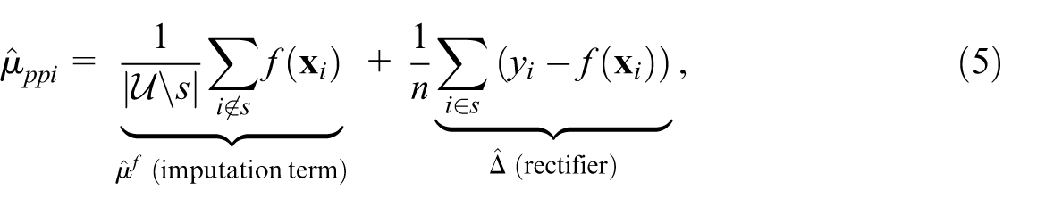
The PPI estimator can be decomposed as
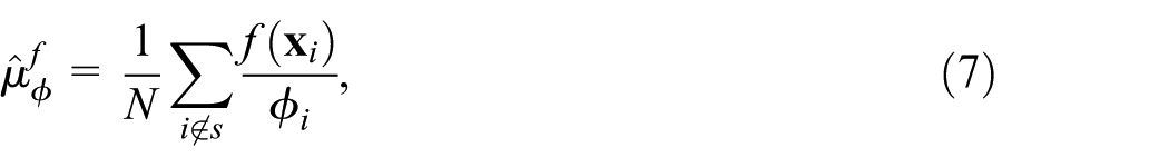
For the imputation term, since PPI does not assume a census of auxiliary data, we must weight the units not selected into the sample. We abstract the survey design as inducing a distribution over partitions of
3.1. Inclusion Probabilities for
Let

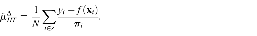
We impose the natural analogue of measurability: (U1)
which is unbiased for
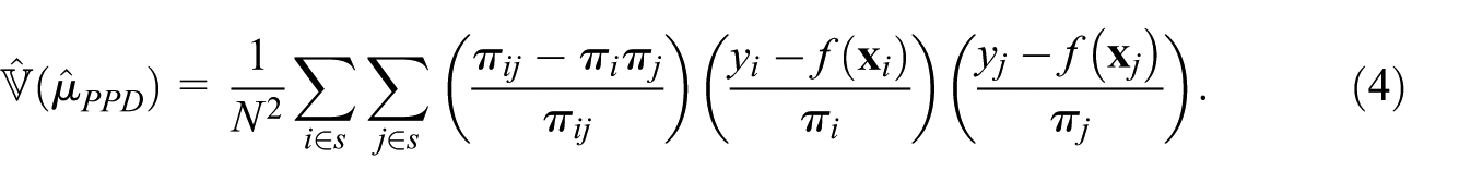
3.2. The PPE Estimator and Its Variance
Combining the two terms, the Prediction-Powered Estimator (PPE) is:
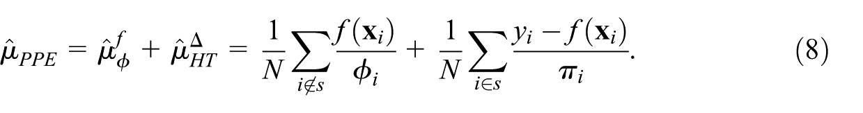
Under assumptions (U1)–(U2) and for any
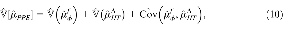
The variance of PPE decomposes as:
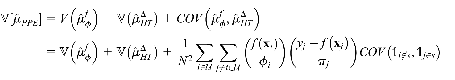
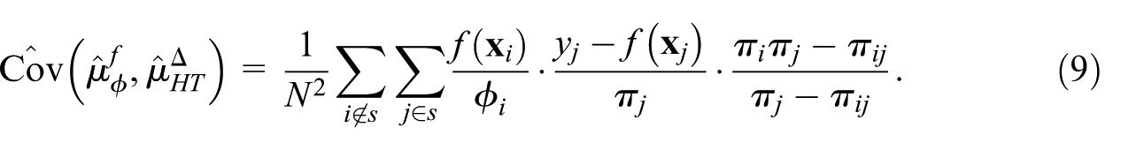
The first two terms are standard HT variances. For the covariance term, noting that:
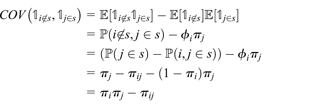
which equals zero for designs with replacement (since
For SRSWOR this simplifies to
where each component is estimated by its standard unbiased HT-type estimator. It holds that
Note that when
Remark A third estimator,
4. LLM Use-Cases
Next, we aim to demonstrate the utility of using pre-trained models in the survey sampling setting by considering two use-cases where LLMs can be leveraged. We select two applications where LLMs can perform extremely well: optical character recognition (OCR), which involves parsing desired text from an image, and coding using harmonized systems, such as the North American Product Classification System (NAPCS). In such scenarios, it is infeasible to utilize model-assisted estimation procedures without a pre-trained model, as the amount of data required to fit such a model far exceeds what is collected in a given survey cycle. Note that no further fine-tuning is performed: we use available LLMs as-is and treat them as pre-trained models.
Specifically, we design two sets of experiments. The first use-case simulates estimating population salary statistics (mean salary). In this setting, we simulate small survey samples and have access to auxiliary data in the form of images of T4 tax forms for the entire population, though the goal of this experiment is to show application to any use-case that can make use of OCR on image data, such as PDFs. The second use-case simulates a Statistics Canada survey that aims to estimate a given population’s grocery spending statistics. For instance, this could be for the purpose of obtaining statistical estimates related to access to fresh and processed foods in a remote location. This use-case simulates a small survey paired with auxiliary data in the form of retail scanner data from grocery retailers over a given time period. Statistics are reported in terms of the NAPCS group, class and subclass hierarchy levels. Published estimates at various NAPCS levels are made. This scenario is highly relevant as many statistical organizations spend large efforts and cost on manually coding data using harmonized systems such as NAPCS and North American Industry Classification System (NAICS).
For both sets of experiments, the data used to train the models (Gemini-2.0-flash, GPT-4.0-mini) are not publicly known. For Section 4.2, the data are artificially generated, so the LLM cannot have been trained on this dataset. While it is not possible to formally distinguish between covariate shift and concept drift in this setting, the document structure and visual layout differ from standard OCR benchmarks, suggesting a form of distributional mismatch relative to the LLM’s pretraining data.
For Section 4.3, the dataset consists of a cleaned subset of a tabular Walmart grocery product dataset. The LLM is used to map short retail product descriptions to NAPCS codes, a task-specific classification problem that reflects the operational context of statistical production rather than general-purpose text understanding. Although similar product descriptions may appear in publicly available corpora, the joint distribution of inputs and target labels induced by this classification task is unlikely to align with the LLM’s pretraining objective. We therefore view this setting as exhibiting a form of task-level distributional shift, consistent with concept drift.
4.1. LLM API Details
Both use-cases rely on commercial LLM APIs. For the T4 salary estimation task (Section 4.2), we use Gemini 2.0 Flash via Google’s Generative AI API (Google 2025). Each API call submits one image alongside a short text prompt and receives a structured JSON response via Pydantic schema enforcement (Pydantic 2025), eliminating the need for post-hoc parsing. At the time of experimentation (early 2025), Gemini 2.0 Flash was priced at approximately USD $ 0.10 per 1,000 image input tokens; processing the full population of
4.2. Salary Estimation with T4 Forms
4.2.1. Methodology
10,000 simulated T4 forms were generated. An automated script was built to generate a wide variety of different T4 forms, rather than using a single T4 template. This was to demonstrate the ability of the LLM to generalize, showcasing the applicability for any use-case where OCR from a diverse range of documents may be of use. First, data for a population unit was generated, which included a name of the individual, a company name, a province, and salary related information. The T4 form box numbers and titles were used as found from the provided T4 template from (Government of Canada 2025c). Several aspects of the data and form generation process were randomized, this included: whether the form was bilingual or not, the font type and size, text coloring, background color, the inclusion of a simple company logo, the layout structure (number of columns, rows), the use of bounding boxes, small rotations, the use of a watermark, image modifications to simulate paper textures, ordering and organization of the T4 boxes/fields. Associated to each generated image was the ground truth salary data. The gross salaries were first randomly sampled, then all related values were randomly generated conditional on this value.
A total of 1,000 Monte Carlo repetitions of a survey were conducted using simple random sampling without replacement (SRSWOR), with a population of size
Point-prediction from the LLM was performed as follows. Briefly, we used the Google API (Google 2025) to call Gemini 2.0-flash (Google DeepMind 2025) which was prompted with a simple text instruction and an image (e.g., see Figure 1), of a T4 form. We enforced a structured response by providing a Pydantic response schema (Pydantic 2025) via the API’s structured response capabilities, thereby ensuring that the text response obtained from Gemini-2.0-flash could be parsed and the returned value would be simply the desired numerical value (float), without any additional text, characters, or explanation.
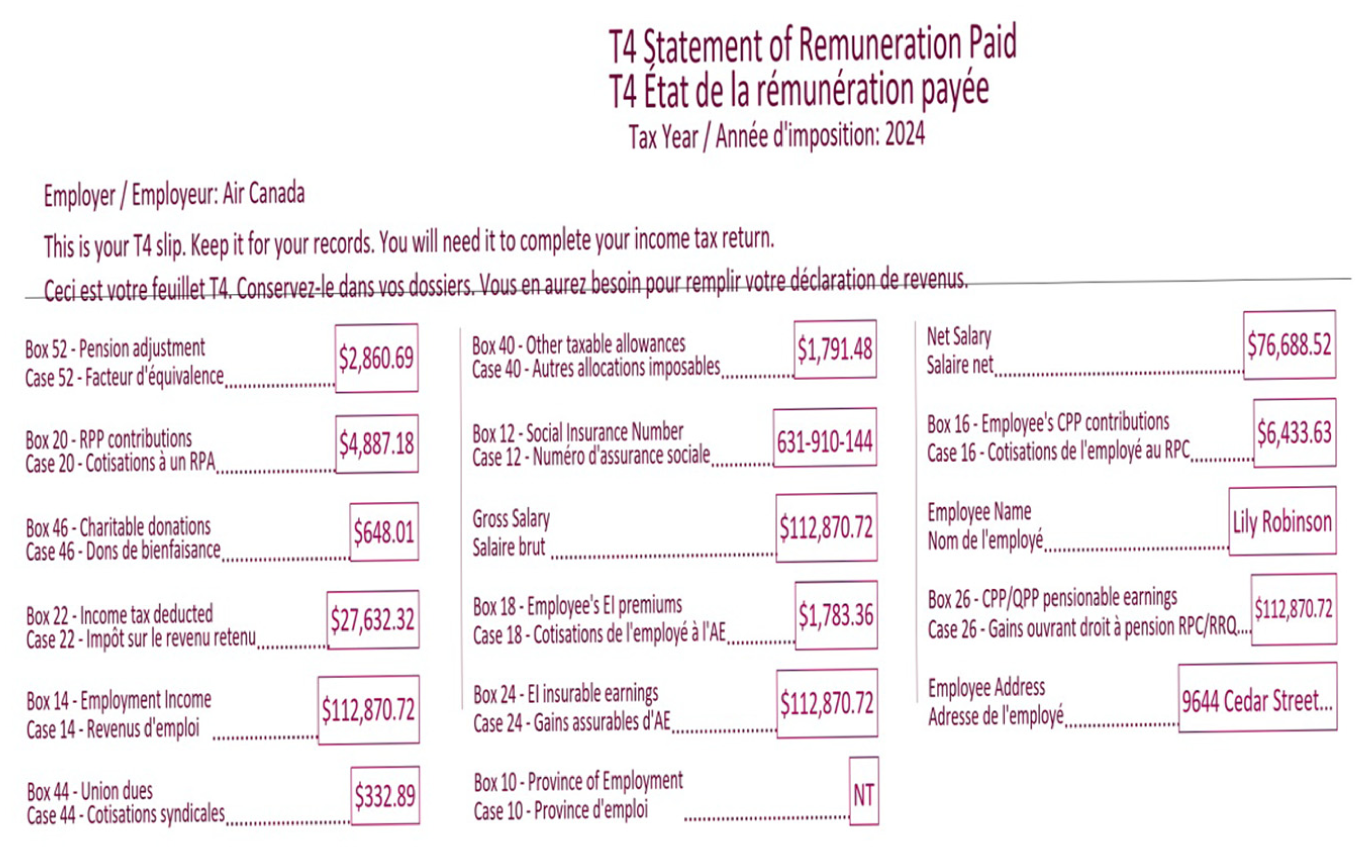
Example of a synthetic T4 tax statement image. Images are generated randomly, with noise and a variety of formats and styles.
4.2.2. Results
We report the relative bias (RB), relative MAE (RelMAE), and relative MSE (RelMSE), as found in Table 1. The results clearly demonstrate the value of using pre-trained models, in the form of LLMs, for this particular use-case, as compared to the HT estimator. Specifically, all three approaches resulted in a mean reduction in MAE between 72.2% and 75.8%, and a mean reduction in MSE between 91.5% and 93.8%, relative to the HT estimator. Of the three proposed approaches, PPE performed slightly behind the others, while
Relative Bias, MAE, and MSE of HT,
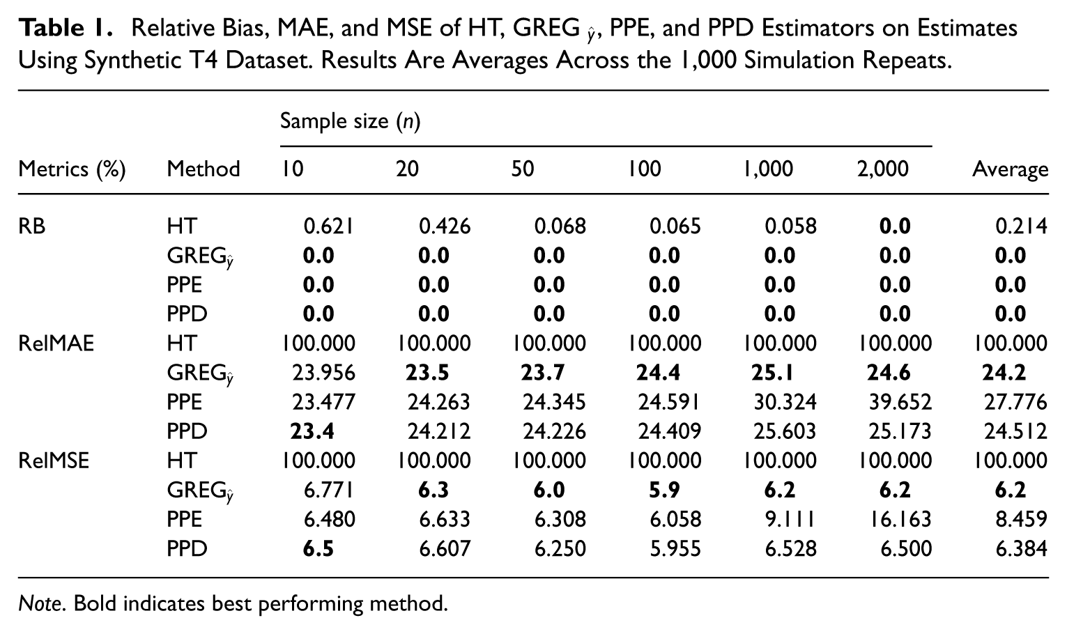
Note. Bold indicates best performing method.
When considering metrics associated to efficiency (see Table 2), the results were fairly consistent. Though the HT estimator did have the highest overall mean coverage (94.4%), the three proposed pre-trained model-assisted estimators performed quite similarly, with coverage ranging from 92.3% to 94.1% (equivalently relative coverage of 97.7%–99.7%). Despite achieving a similar coverage rate to the HT estimator, the proposed approaches did so much more efficiently, with a reduction in CI width ranging from 74.3% to 77.7%, relative to the HT estimator. The Relative MSE
Relative Efficiency Metrics of HT,
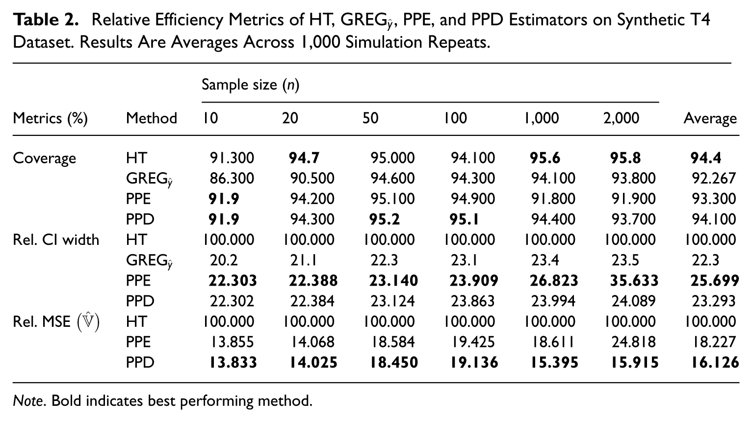
Note. Bold indicates best performing method.
We perform HT-equivalent sample size experiments as a means of highlighting potential real-world efficiency gains, where the HT-equivalent sample size is defined as the smallest sample size that a given model-assisted estimator requires to achieve the same estimation accuracy as the HT estimator at a given reference sample size. Compared to the HT estimator with a sample size of
4.3. NAPCS Grocery Dataset
In these experiments, the aim is to simulate a setting where the goal is to produce household grocery spending estimates associated to product categories of a given NAPCS code level. The publicly open Walmart Grocery Product Dataset (Kaggle 2025) was used and adapted for these studies. This dataset comprises of information regarding products sold from US Walmart Grocery Departments. The data includes the grocery department (e.g., deli), the category (e.g., Hummus, Dips, and Salsa), the product name (e.g., Marketside Roasted Red Pepper Hummus, 10 oz), and the price in USD. We treat the dataset as a proxy of a retail scanner dataset, and treat the product names and prices as retail scanner data.
4.3.1. Methodology
The Walmart Grocery Product Dataset (Kaggle 2025) was processed to remove unnecessary columns and remove duplicate data. The dataset does not come with any ground truth NAPCS codes. We implement an LLM coder to provide target labels for these experiments. For this approach we implement a labeling pipeline. Briefly, we use Google’s API to prompt Gemini-2.0-flash with instructions on the task, provide it with a list and description of 17 pre-filtered NAPCS-3 level (group) codes associated to food and beverages and have the LLM return the top-3 most likely NAPCS-3 level codes associated to the input product data. We call these the predicted groups. Next, we retrieve all the NAPCS-5 level (class) codes associated to the predicted groups, which range from 1 to 16 classes per group. Again, we provide the LLM with instructions on the task, the list of potential classes (with descriptions) and query the LLM to respond with the top-5 most likely classes. Next, we collect all the NAPCS-6 level (subclass) codes associated to the predicted classes, which range from 1 to 51 subclasses per class. We provide the LLM with instructions on the task, the list of potential subclasses (with descriptions) and query the LLM to respond with the single most likely subclass. We use Pydantic (Pydantic 2025) and structured responses to ensure conformity with desired outputs. We treat these LLM provided codes as the target ground truth NAPCS codes for the remainder of the experiments. We do not assert that these are the ground truth NAPCS codes for the data, but assume they are a noisy proxy and useful for research purposes.
To acquire point-predictions from a pre-trained model, we use a similar approach as described for the LLM-coder, however we use GPT-4o-mini from OpenAI (OpenAI 2024). In contrast to the above approach for the LLM-coder, after receiving the class-level predictions and filtering the feasible set of subclasses, we instead query the LLM to respond with the top-10 most likely NAPCS-6 level (subclass) codes. With the top-10 most likely NAPCS-6 level codes, we prompt the LLM one last time and frame the question as a multiple choice question, with each of the 10 possible subclasses associated to multiple choice options: A-J. We prompt the LLM to respond with a single token response, A through J, and receive the log-probabilities of the response from the API, which we convert to probability scores. We assign a probability score of 0 to all subclasses outside this top-10. Once the dataset has been processed, we perform a calibration procedure where we sample 10% (≈ 3,000) of the data and use isotonic regression (Niculescu-Mizil and Caruana 2005; scikit-learn 2025b) to perform probability calibration across all subclasses. At this stage of the model’s point-prediction we can associate to each input instance a probability vector over NAPCS-6 subclasses, which is then multiplied by the product price. One can also view this approach as a set of C point-prediction models, one for each of the C NAPCS-6 subclasses.
1,000 Monte Carlo repeats of a survey were conducted using SRSWOR using a population of size
The HT estimator was compared to the PPE, PPD, and
4.3.2. Result
Aggregated across all NAPCS-6 subclasses, sample sizes, and experimental repeats, PPD and PPE consistently outperform HT across all metrics considered. Both estimators achieved higher mean and median coverage than HT, and for nearly every other metric computed—MAE, MSE, CI width, CV, and coverage error—PPD and PPE yielded approximately a
Summary of Metrics for NAPCS Codes at Sample Size
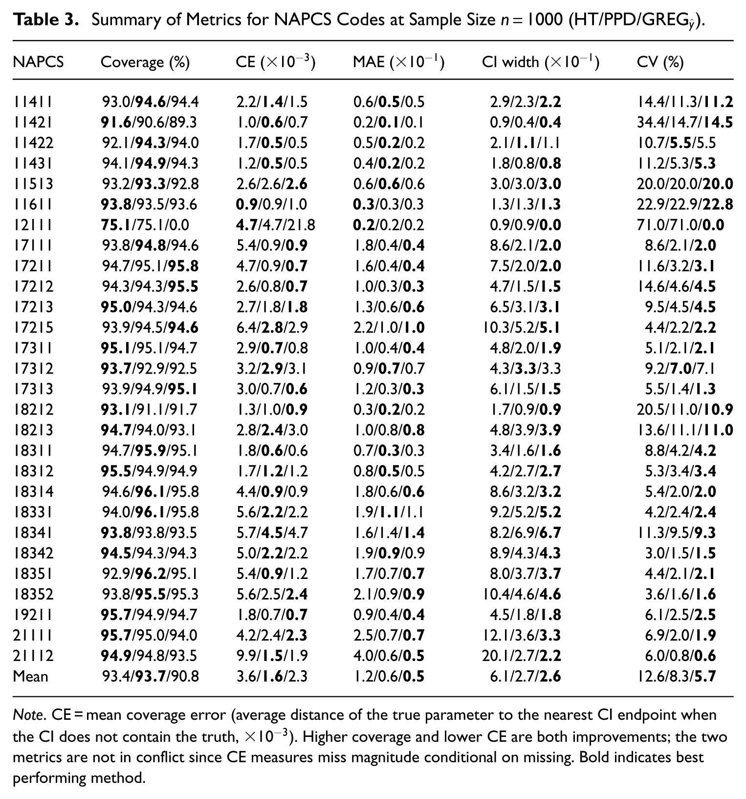
Note. CE = mean coverage error (average distance of the true parameter to the nearest CI endpoint when the CI does not contain the truth,
HT-equivalent sample size experiments were performed, where again HT-equivalent sample size is defined as the smallest sample size that a given model-assisted estimator requires to achieve the same estimation accuracy as the HT estimator at a given reference sample size. Figure 2 shows the HT-equivalent sample size of NAPCS-5 class-level estimates, reported relative to the HT estimator with sample size
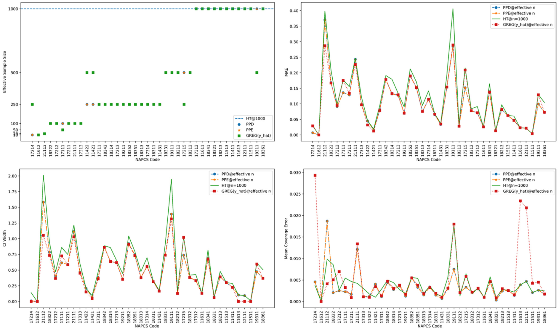
HT-equivalent sample size experiments for PPE, PPD, and
Across each NAPCS-5 class, the estimates produced by PPE and PPD are more precise and more efficient than the HT estimator at n = 1,000, even when using smaller sample sizes in 27/39 of the estimates. Though
The
5. Real-World Dataset
In this section, we apply PPD to real-world data collected by Statistics Canada, Canada’s national statistical organization. The Quarterly Survey of Financial Statements (QSFS) collects data used to measure the financial position and performance of incorporated businesses within Canada (Government of Canada 2025b). The data includes items related to assets, liabilities, and equity within a quarterly balance sheet, revenue and expense data reported on a quarterly income statement. The survey is collected quarterly, with a population frame size of approximately 28,000 enterprises. Sampling is carried out using a stratified random sample, with strata constructed based on the size of the unit (assets). Sample sizes are typically around 5,000 units.
The auxiliary data considered includes monthly tax (GST) data and General Index of Financial Information (GIFI) data (Government of Canada 2025a), the previous year’s annual revenue and annual assets within Statistics Canada’s internal Business Register. As well, relatively static administrative data is available for each unit, with information related to the size of the enterprise, the industry that the enterprise is classified under, as well as the North American Industry Classification System (NAICS) code associated to that enterprise. For the GST variables, for each quarter, the GST tax data available includes the GST for the first and second month of that quarter. GIFI codes are associated to particular items found on a corporation’s financial statements (e.g., balance sheets, income statements, and statements of retained earnings). However, there is approximately a two-year lag in the availability of the GIFI data, relative to a given survey quarter. These covariates are used for model fitting and point-predictions at survey time.
5.1. Methodology
For these experiments, quarterly QSFS survey data was available for 11 quarters, from 2022-Q1 to 2024-Q3. For each target quarter, we fit a gradient boosting regression model (Friedman 2001; scikit-learn 2025a) using the full survey data from the immediately preceding quarter (approximately
We ran simulations over the 2022-Q2 to 2024-Q3 quarters (ten quarters total). For each quarter, the full survey data was treated as a population frame and SRSWOR was performed for sample sizes
5.2. Results
High-level aggregate results across all sample sizes, survey quarters, and experimental repeats are shown using violin plots in Figure 3. Relative
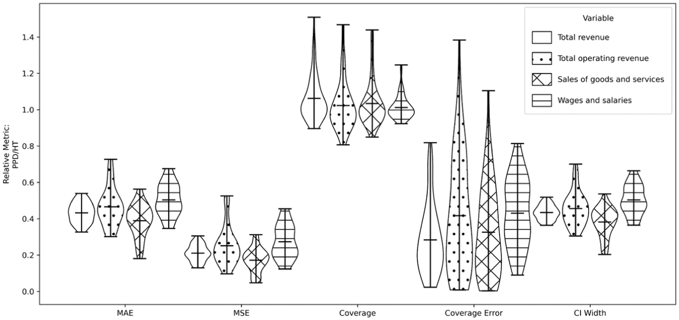
Aggregated relative performance of PPD versus HT estimators across various metrics over ten QSFS survey quarters for four survey response variables (see legend).
We explore the HT-equivalent sample sizes for the QSFS variables, defined as the smallest sample size that the PPD estimator requires to achieve the same estimation accuracy as the HT estimator at
Figure 4 shows the HT-equivalent sample size (top left) for each survey variable across the QSFS survey quarters (
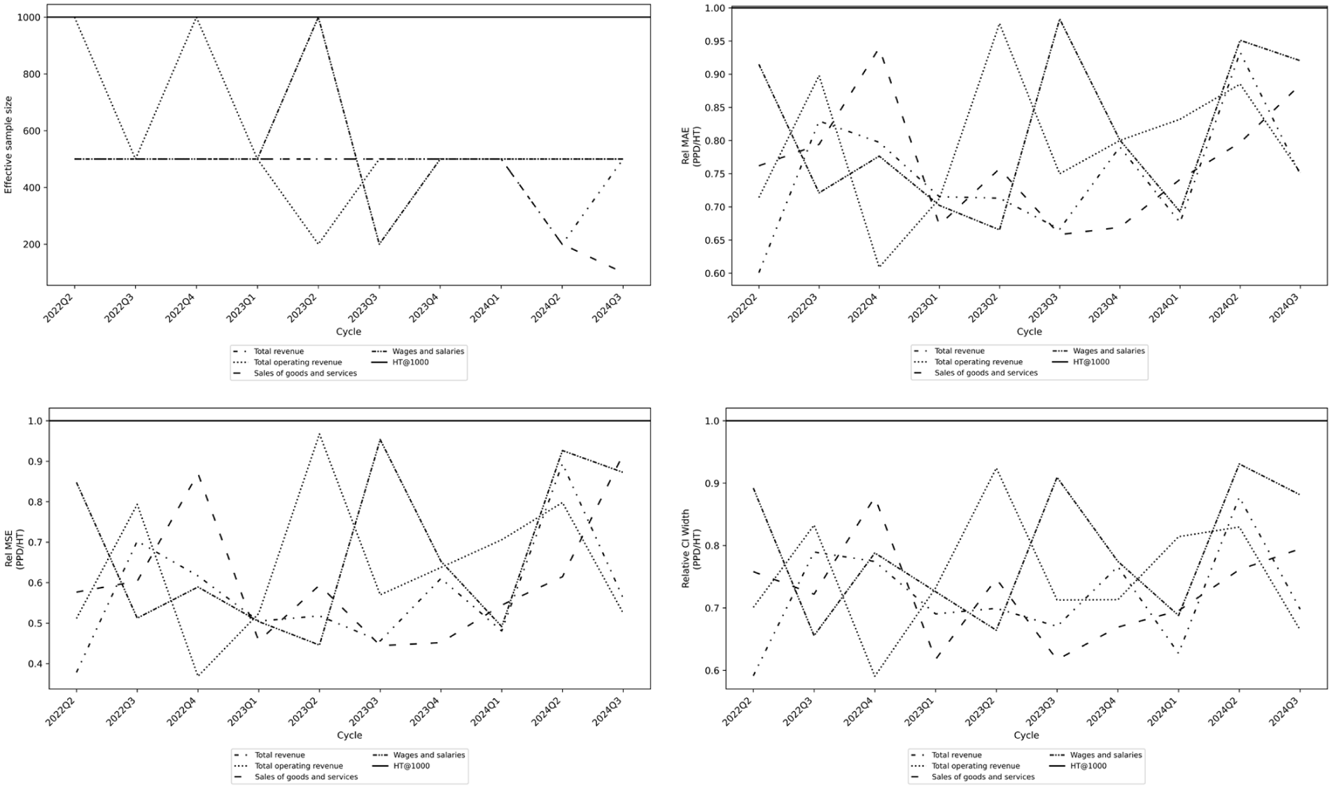
HT-equivalent sample size for QSFS variables (PPD vs. HT@
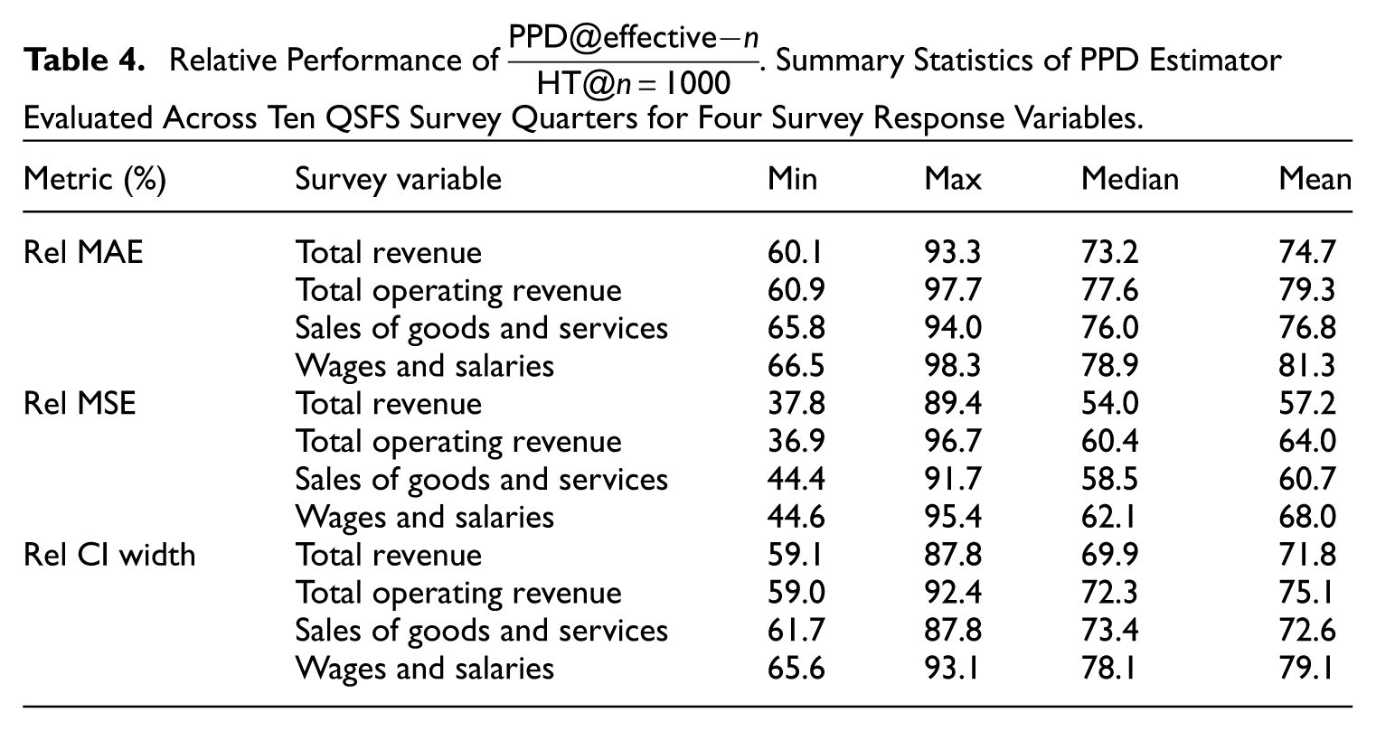
For each survey response variable we report summary statistics on the relative metrics (Table 4) across the survey quarters. Here, the relative metrics are reported with respect to
Relative Performance of
6. Discussion
This work examined the use of pre-trained black-box models for survey estimation. Despite the difference estimator and
We considered three estimators that make use of pre-trained models: PPE, as a direct extension of PPI to survey settings; the Prediction-Powered Difference (PPD) estimator, as a re-framing of the generalized difference estimator (Cassel et al. 1976) when a pre-trained model is used; and
Through LLM-based experiments (Section 4) and real-world QSFS experiments (Section 5), the proposed approaches consistently outperformed HT and, where applicable, GREG and MC baselines across a range of sample sizes. The simulation experiments (Supplemental Material) corroborate these findings across a range of controlled data-generating processes. HT-equivalent sample size analyzes suggest that these approaches could contribute to partial reductions in survey sample sizes and respondent burden, though the magnitude of gains will depend on the quality of the pre-trained model and the degree of distributional shift between training and survey data.
The simulation results (Supplemental Material) highlight a fundamental limitation of MC estimation with non-linear models: because the variance is estimated from the residuals of the same data used to fit the model, overfitting produces misleadingly small residuals and severely underestimated variance, resulting in poor coverage—on average just above 10% in the simulations. By contrast, PPE and PPD use residuals evaluated on the survey sample, which is independent of model training, yielding unbiased variance estimates. This distinction is practically important as survey sample sizes decrease and non-response increases, making asymptotic justifications for MC and GREG less reliable.
The results also illustrate that when auxiliary data has a non-linear relationship with the target variable—which is the case for most unstructured data sources—linear model-assisted approaches are insufficient, while pre-trained non-linear models used via PPD, PPE, or
The performance of the proposed estimators depends directly on the quality of the pre-trained model. In the experiments presented here, no domain-specific model development was undertaken beyond generic hyperparameter tuning (Optuna 2024), and no prompting strategies were optimized for the LLM-based tasks. Results should therefore be interpreted as indicative rather than as an upper bound on achievable performance; targeted model development in a production setting may yield different results depending on the application.
Whether PPD and PPE outperform unbiased or consistent model-training alternatives—such as the SRB estimator of Sanguiao-Sande and Zhang (2021)—in specific survey settings remains an open question and a direction for future work. Additional promising directions include the application of PPE and PPD under more complex survey designs, and the use of pre-trained model predictions to inform strata allocation in stratified random sampling (Godfrey et al. 1984).
These results do not argue that model-assisted techniques which fit models using survey data should be abandoned. Rather, the survey methodologist should consider both in-sample and pre-trained model approaches for their particular use-case, selecting the one most appropriate to the setting, the available auxiliary data, and the model classes that are feasible given the sample size.
Calibration-based refinements of PPD (Prediction-Powered Model-Calibration Estimator), such as using pretrained predictions as calibration variables to enforce agreement between sample-weighted and population prediction totals—in the spirit of the model-calibration framework of Wu and Sitter (2001)—represent a natural extension that may offer additional robustness to systematic prediction bias, and merit further investigation.
Supplemental Material
sj-docx-1-jof-10.1177_0282423X261451320 – Supplemental material for Prediction-Powered Estimation: Unbiased Model-Assisted Estimation
Supplemental material, sj-docx-1-jof-10.1177_0282423X261451320 for Prediction-Powered Estimation: Unbiased Model-Assisted Estimation by Nicholas Denis and Mohammed Haddou in Journal of Official Statistics
Footnotes
Acknowledgements
The authors would like to acknowledge: Jean-Francois Beaumont, Keven Bosa, and Steve Matthews for reviewing and providing helpful feedback on manuscript drafts, and Ivy McKee for help processing QSFS data and providing helpful background information on the QSFS survey.
Funding
The authors received no financial support for the research, authorship, and/or publication of this article.
Supplemental Material
Supplemental material for this article is available online.
Received: May 23, 2025
Accepted: April 15, 2026
References
Supplementary Material
Please find the following supplemental material available below.
For Open Access articles published under a Creative Commons License, all supplemental material carries the same license as the article it is associated with.
For non-Open Access articles published, all supplemental material carries a non-exclusive license, and permission requests for re-use of supplemental material or any part of supplemental material shall be sent directly to the copyright owner as specified in the copyright notice associated with the article.