
Abstract
The gamma distribution is a useful model for small area prediction of a skewed response variable. We study the use of the gamma distribution for small area prediction. We emphasize a model, called the gamma-gamma model, in which the area random effects have gamma distributions. We compare this model to a generalized linear mixed model. Each of these two models has been proposed independently in the literature, but the two models have not yet been formally compared. We evaluate the properties of two mean square error estimators for the gamma-gamma model, both of which incorporate corrections for the bias of the estimator of the leading term. Finally, we extend the gamma-gamma model to informative sampling. We conduct thorough simulation studies to assess the properties of the alternative predictors. We apply the proposed methods to data from an agricultural survey.
1. Introduction
Response variables of interest in applications are often positive and have asymmetric distributions. Examples documented in the fields of health, economics, and agriculture include the body mass index (Pfeffermann and Sverchkov 2007), income (Molina and Rao 2010), and sheet and rill erosion (Berg and Chandra 2014). These types of data are often used to gain a deeper understanding of the characteristics of sub-populations (sub-domains) defined by geographic regions or socio-demographic groups. Such subdivisions are usually granular and therefore have sample sizes that are small or even zero. This motivates the definition of a small area (domain) as any sub-population where the area-specific data are insufficient to assure direct domain estimates of acceptable precision. Estimation procedures for small domains commonly employ indirect estimators based on small area models that incorporate between-area variation and auxiliary variables (Jiang and Lahiri 2006; Morales et al. 2021; Pfeffermann 2013; Rao and Molina 2015). A fundamental small area model is the unit-level linear mixed model of Battese et al. (1988). This model assumes normal distributions and is not immediately suitable for positive, skewed data.
A common approach for skewed data is to apply the unit-level linear mixed model of Battese et al. (1988), after an appropriate transformation. In the framework of a unit-level lognormal model, Berg and Chandra (2014) develop closed-form expressions for an empirical Bayes predictor of a small area mean. Lyu et al. (2020) and Zimmermann and Münnich (2018) extend the lognormal model to zero-inflated data and informative sampling, respectively. Berg and Chandra (2014), Lyu et al. (2020), and Zimmermann and Münnich (2018) focus on prediction of means, but many small area parameters are more complex functions of the model response variable. Molina and Rao (2010) obtain a Monte Carlo (MC) approximation for the best predictor of a general small area parameter, assuming that the nested error linear regression model holds after a transformation of the response variable. Guadarrama et al. (2018) develop predictors of general small area parameters under an informative sample design. Rojas-Perilla et al. (2020) extend Molina and Rao (2010) to data-driven transformations that are more general than the log transformation. Though widely used, transformations have drawbacks. As noted in Graf et al. (2019), log transformed response variables often exhibit skewness relative to a normal distribution, and finding a suitable transformation can be difficult.
An alternative to a transformation is to model the response variable directly. The gamma distribution enables the analyst to model skewed data in the original scale, without need for a transformation. Hobza et al. (2020) compares several small area predictors, developed under a generalized linear mixed model (GLMM) with a gamma distributed response variable. A challenge with the gamma GLMM is that the likelihood and empirical best (EB) predictors involve intractable integrals. Dreassi et al. (2014) use Bayesian inference procedures to construct small area estimates under the assumptions of a gamma GLMM. Berg et al. (2016) compare predictors based on lognormal and gamma distributions through simulation, and find that the predictors based on the gamma distribution seem more robust to model misspecification. Graf et al. (2019) develop empirical best small area predictors of both means and more general small area parameters under the assumptions of a generalized gamma inverse-gamma distribution. Unlike the gamma GLMM, the model of Graf et al. (2019) leads to tractable integrals and predictors with closed-form expressions. The works of Hobza et al. (2020) and Graf et al. (2019) provide the impetus for the research in this paper.
We study small area predictors based on gamma distributions. We focus on a unit-level model with a gamma response distribution and gamma distributed random effects, which we call the “gamma-gamma” model. The gamma-gamma model is a special case of the more general model of Graf et al. (2019), with a slightly different parametrization. We compare predictors based on the gamma-gamma model to the predictors based on the gamma GLMM. An important innovation of this work is that we develop predictors for the gamma-gamma model as well as estimators of their prediction errors in the context of an informative sample design. Our approach to informative sampling transfers the fundamental concepts of Pfeffermann and Sverchkov (2007) to the gamma-gamma framework.
Although the models in this paper are not new, our work has several important contributions. First, the extension of the gamma-gamma model to informative sampling is the most substantive contribution because Graf et al. (2019) only consider noninformative designs. Second, we formally compare predictors based on the gamma-gamma model to predictors based on the gamma GLMM through simulation. Graf et al. (2019) only compare their model to a lognormal model, and Hobza et al. (2020) exclusively consider the gamma GLMM. We evaluate the robustness of the predictors by simulating data from both the gamma-gamma model and the gamma GLMM. Our third contribution is in the area of mean square error (MSE) estimation. We evaluate the properties of several MSE estimators for the gamma-gamma model through simulation. We also propose an MSE estimator that has not yet been used in combination with the gamma-gamma model. This MSE estimator differs from the estimator of Graf et al. (2019). Graf et al. (2019) use a standard parametric bootstrap MSE estimator. In contrast, we decompose the MSE as a sum of two terms and estimate the two terms in the MSE directly. Note that although Graf et al. (2019) propose an MSE estimator, they do not evaluate its properties through simulation. We also innovate on the MSE estimator of Graf et al. (2019) by applying a bootstrap bias correction to the MSE estimator of Graf et al. (2019) and extending them to informative sampling. Our final two contributions are relatively minor but are valuable nonetheless. We develop predictors for the gamma-gamma model using a hierarchical formulation that is computationally easier to implement than the formulation based on marginal distributions in Graf et al. (2019). Finally, we generalize the procedures of Hobza et al. (2020) to prediction of small area parameters that are more general than the class of additive small area parameters. Hobza et al. (2020) define predictors for additive small area parameters of the form
The procedures discussed in this paper are relevant to studies of sheet and rill erosion, or soil loss due to the flow of water. Small area estimates of sheet and rill erosion are valuable for assessing the efficacy of conservation programs. Sheet and rill erosion is positive, and past studies (Berg and Chandra 2014; Lyu et al. 2020) have documented the distribution of sheet and rill erosion to be skewed right. The data on sheet and rill erosion are derived from large-scale surveys that use complex designs. Therefore, the predictors that we develop for informative sampling in the context of the gamma distribution are imperative for the application to small area estimation of sheet and rill erosion.
Our study of small area prediction based on gamma distributions is organized as follows. In Section 2, we define the gamma-gamma model and the gamma GLMM. In Section 3, we propose two MSE estimators for the gamma-gamma model. In Section 4, we extend the gamma-gamma model to an informative sample design. In Section 5, we present simulation studies that (1) compare the gamma-gamma model to the gamma GLMM and (2) evaluate the alternative MSE estimators. The data analysis is presented in Section 6. We summarize the main conclusions in Section 7.
2. Small Area Estimation Based on Gamma Distributions
We establish a common notation that we will use for both the gamma-gamma model and the gamma GLMM. Let

where
A critical assumption of our procedure is that the covariate
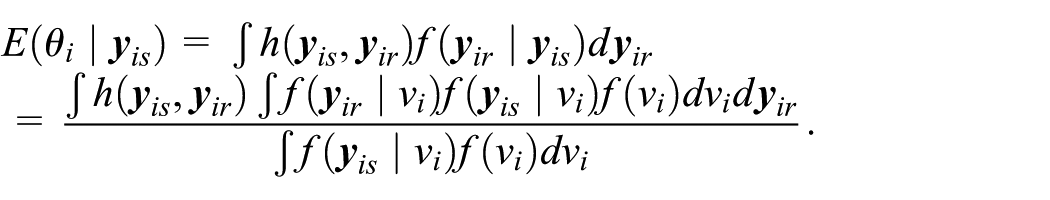
Suppose a population model is specified for y ij , and let E p denote expectation with respect to the population distribution. Under the model, the minimum mean square error predictor of θ i is defined as

which is called the best predictor (BP) of the area parameter. In this section, we develop best predictors of θ i under two models that assume a gamma distribution for the response variables. Section 2.1 and Section 2.2 describe the gamma-gamma model and the gamma GLMM, respectively.
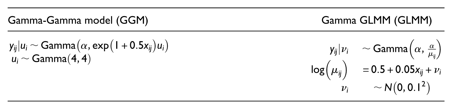
2.1. Unit-Level Gamma-Gamma Small Area Model
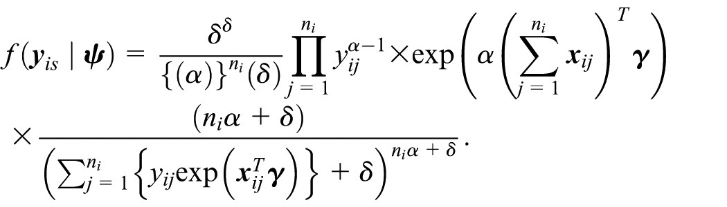
Assume that the population is generated under a gamma-gamma small area model defined as

where
We first consider small area prediction of the mean defined as

Theorem 1 gives the best predictor of
A proof of Theorem 1 is given in the Supplemental Material. We use the notation
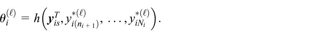
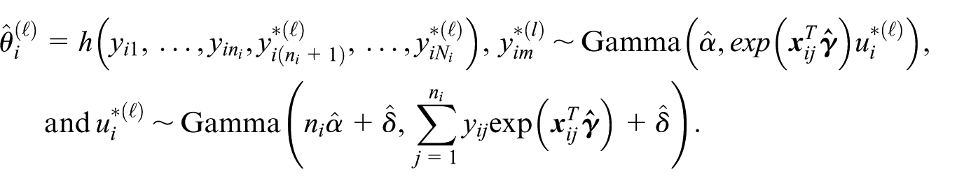
We next consider prediction of more general small area parameters of the form in Equation (1). Depending on the complexity of the real-valued function

This convenient form for the distribution of u
i
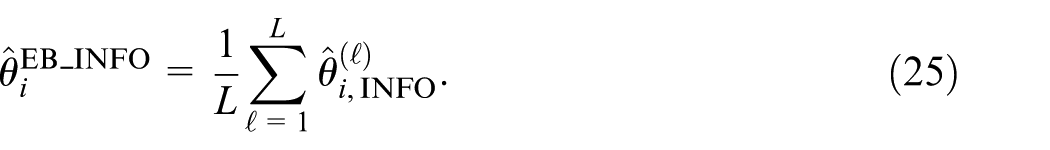
enables us to develop a simple algorithm for approximating the best predictor of θ
i
. For
Generate
Generate
Define
An approximation for the best predictor of the area parameter is defined as

The notation
The algorithm above is slightly simpler than the algorithm of Graf et al. (2019). We exploit the convenient form of the conditional distribution of u
i
to generate y
ij
for nonsampled elements through a hierarchical process that involves first generating u
i
and then generating y
ij
given u
i
. In contrast, Graf et al. (2019) generate y
ij
from the marginal distribution of
The best predictor is a function of the unknown model parameters, denoted as

where
A proof of Theorem 2 is given in the Supplemental Material. Let

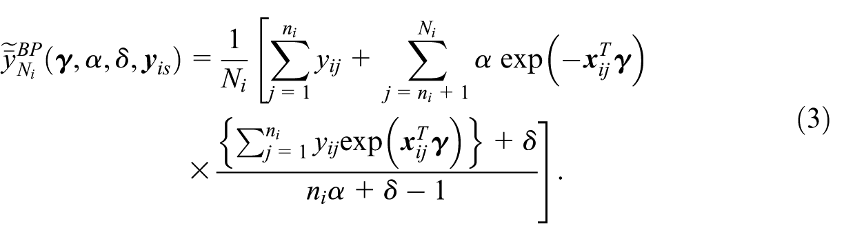
Given the maximum likelihood estimator, we define an empirical best (EB) predictor by substitution of
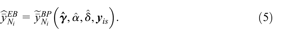
The predictor Equation (5) is obtained by evaluating the closed-form expression for the best predictor of the mean in Equation (3) at the maximum likelihood estimators. To define an empirical best predictor of a general small area parameter, we repeat steps 1 to 3 above with the maximum likelihood estimators in place of the true model parameters. This enables us to define the EB predictor of a general small area parameter by

where
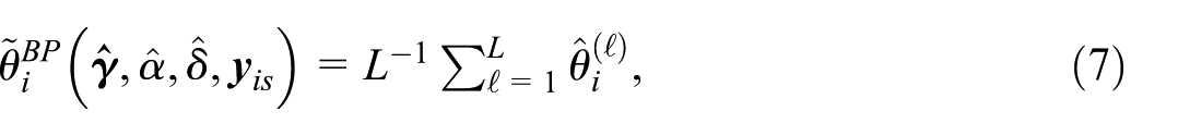
We refer to the predictor Equation (6) as the EB predictor. When we use the EB predictor Equation (6) to predict the mean, we obtain an MC approximation for the closed-form predictor Equation (5).
2.2. Gamma GLMM
Define a unit-level gamma GLMM by
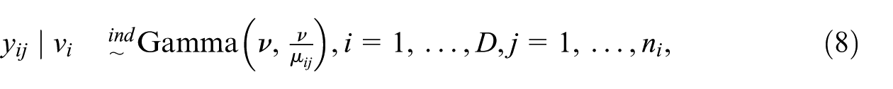
where
Note that the best predictor of θ i can be expressed as a ratio of two integrals:
The integrals do not have closed form expressions. We use sampling importance resampling (Smith and Gelfand 1992) to approximate the integrals. The iterative Monte Carlo algorithm is as follows:
For
(a) for
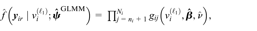
and
(b) Calculate
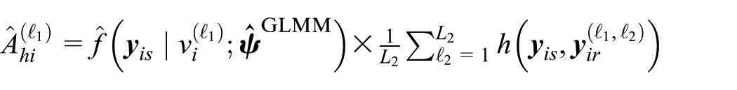
and
(c) Define the EB predictor of θ i as
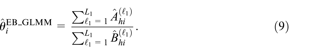
Note that the predictor defined in Equation (9) is an empirical best predictor under the GLMM, while the predictor defined in Equation (6) is an empirical best predictor under the gamma-gamma model. Both predictors are empirical best predictors, but they are constructed under different model assumptions.
Another predictor, referred to as the plug-in predictor, is defined as

where
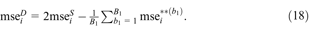
3. MSE Estimation
In this section, we define two estimators of the MSE of
3.1. Proposed MSE Estimator
Suppose we use

where
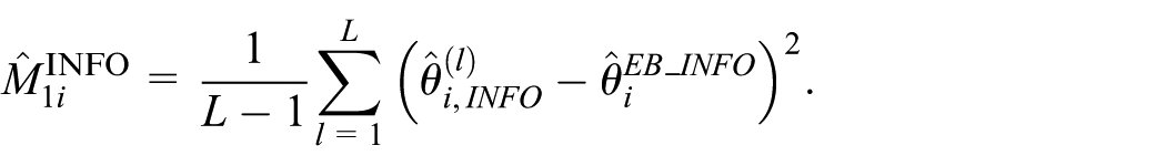
The first term Mi1, called the leading term, is the MSE of the best predictor, and its unbiased estimator is
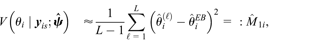
where
The extra variation induced by replacing
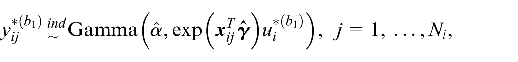
Generate the bootstrap sample
Estimate the bootstrap version of the model parameter estimates,
Calculate the bootstrap predictor,
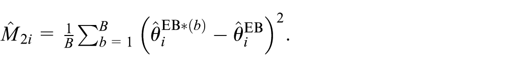
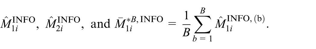
Then, define the estimator of M2i as:
A preliminary estimator of the MSE of θ i is defined as

The label “noBC” is used to indicate that the MSE estimator Equation (12) does not incorporate a correction for the bias of the estimator of the leading term.
However, the estimator of leading term


These classic additive and multiplicative bias-correction approaches are straightforward, but Hall and Maiti (2006) mention several issues with those approaches. The additive and multiplicative bias-correction could produce a negative leading term estimator when
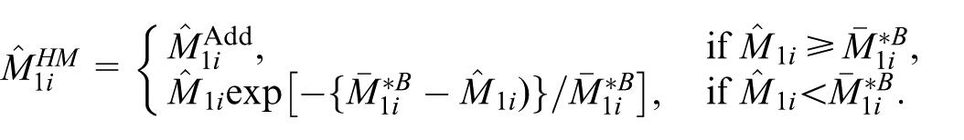
As a special case of the general bias corrections given in Hall and Maiti (2006), we further define a compromise between
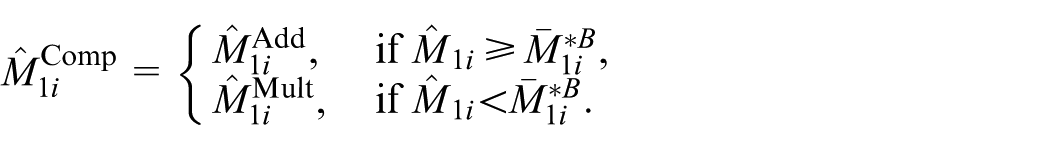
In summary, the bias-corrected MSE estimators are constructed by

and

3.2. Existing Parametric Bootstrap MSE Estimators
Instead of estimating Mi1 and Mi2 separately, one can use the parametric bootstrap to estimate
Obtain the maximum likelihood estimate of the model parameter
For
where
3. Calculate the bootstrap version of a small area parameter as
4. (a) For
(We set B 2 = 1 to employ the simpler double-bootstrap.)
(b) Calculate the bootstrap version of a small area parameter
(c) Set
5. Finally, define the single-stage and the double-bootstrap MSE estimators as

and
Note that the single-stage MSE estimator is comparable to Equation (12) and the (simpler) double-stage MSE estimator to the proposed bias-corrected MSE estimators.
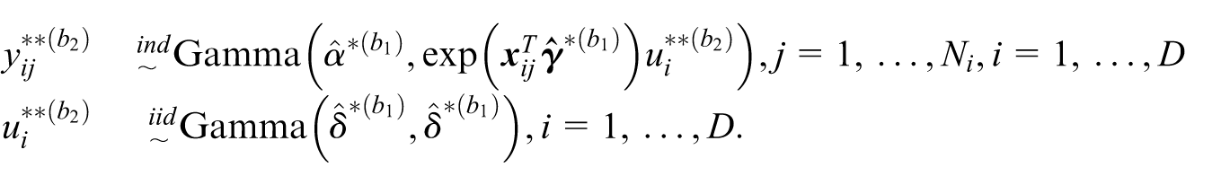
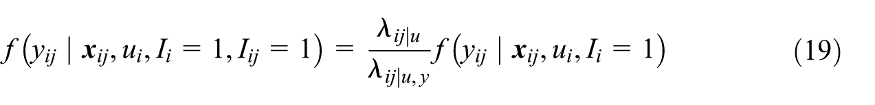
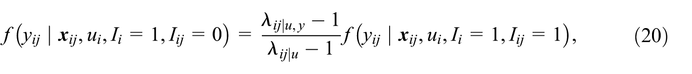
4. Extension of SAE Gamma-Gamma Model Under Informative Sampling
We extend the gamma-gamma model to an informative sampling design. We utilize well-known relationships among the population, sample, and sample-complement distributions of y ij established in Pfeffermann and Sverchkov (2007). We assume the same model for the first moment of the sampling weight in Pfeffermann and Sverchkov (2007). Our approach differs from that of Berg and Eideh (2024) because we derive the exact complement distribution instead of the population distribution.
For completeness, we restate key relationships defined in Pfeffermann and Sverchkov (2007) with respect to the second-stage unit y ij and the corresponding sampling weight as w ij . These are given by
and
where I
i
and I
ij
are the sample indicators for area i and unit j within area i, respectively;
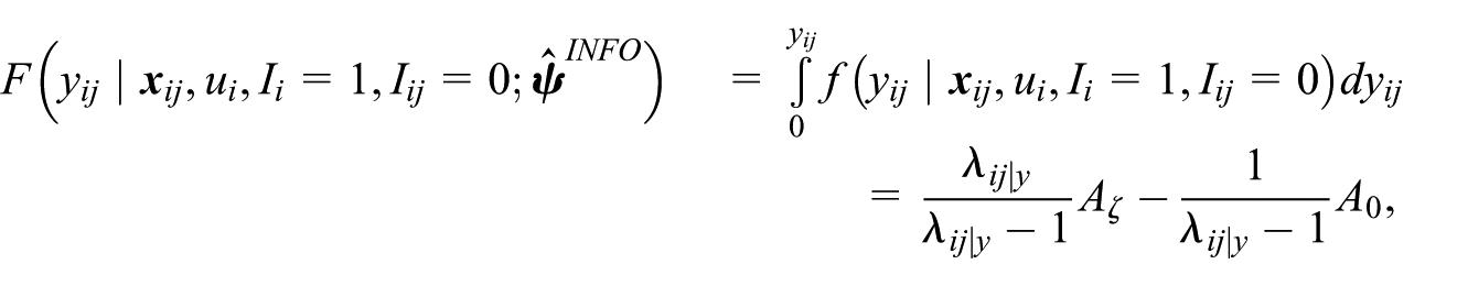
For the complex design, we suppose the sample distribution is given by

where
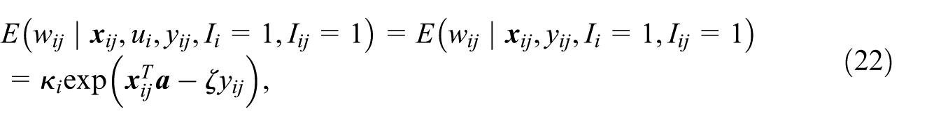
for ζ > 0 where
where
When the observed values are not related to sampling probability (i.e., ζ= 0), the population and sample-complement distribution,
However, under the informative design, that is

as in Pfeffermann and Sverchkov (2007). The procedure for the best predictor under the informative design is then implemented as follows. For
Generate
Generate
Define

Then, the empirical best predictor of the area parameter is defined as
Generate
Set
Based on the mean weight model in Equation (22), we extend the MSE estimators from Section 3.1 to quantify the prediction error associated with
However, because the weight model in Equation (22) is specified only through its first moment, a fully parametric bootstrap procedure is not directly feasible for estimating the second component M2i (Berg and Eideh 2024). To account for the variability induced by replacing the fixed model parameters with their estimates in the predictor, we adapt the procedure proposed by Cho and Berg (2022) within our framework:
Compute the jackknife variance estimator for
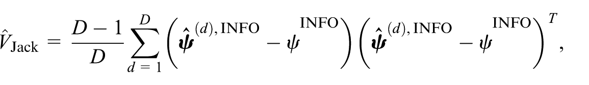
where
For
Calculate the estimator of the second component as:

Then, the MSE estimator without the bias-correction for
Then, denoted them as
5. Simulation Study
5.1. Simulation Study 1: Comparison of Predictors
We evaluate the performance of gamma-gamma predictors introduced in Sections 2 and 4 under multiple scenarios. We modified the simulation setup of Pfeffermann and Sverchkov (2007) tailored to our framework. For each scenario, we consider D= 60 areas, each with population size N
i
= 1000 and stratify the areas into two strata, where Stratum H1 and Stratum H2 are composed of areas
In this simulation study, we further examine the robustness of the gamma-gamma predictors against model misspecification. Each scenario is generated from a combination of the population model for a response variable y with skewness being adjusted through the shape parameter in a gamma distribution (α) and the inclusion probability π
ij
model with whether an informative sampling design is used (
Population model for y, with
Inclusion probability π
ij
model for systematic sampling,
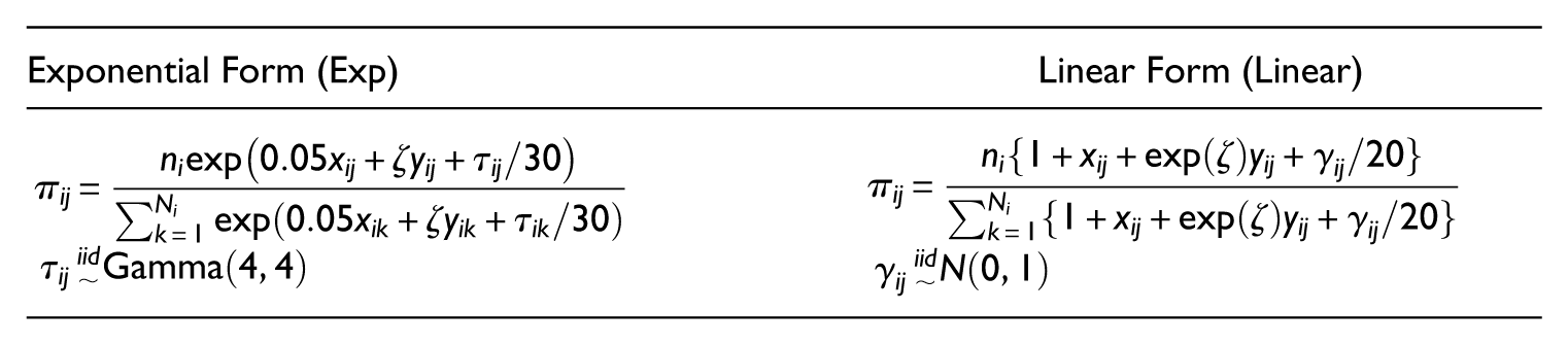
Note that the skewness of the distribution decreases as α increases, and we set
For a given scenario, in the m-th MC iteration,
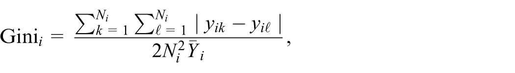
where the value is obtained by the function gini of R package reldist (Handcock 2023).
We compare the predictors using the relative bias (RB) and RRMSE. The RB and RRMSE for the predictor “pred” are defined as
where
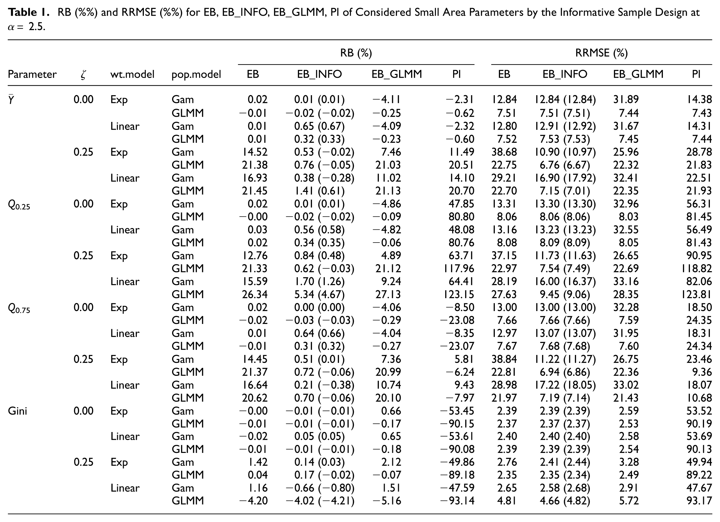
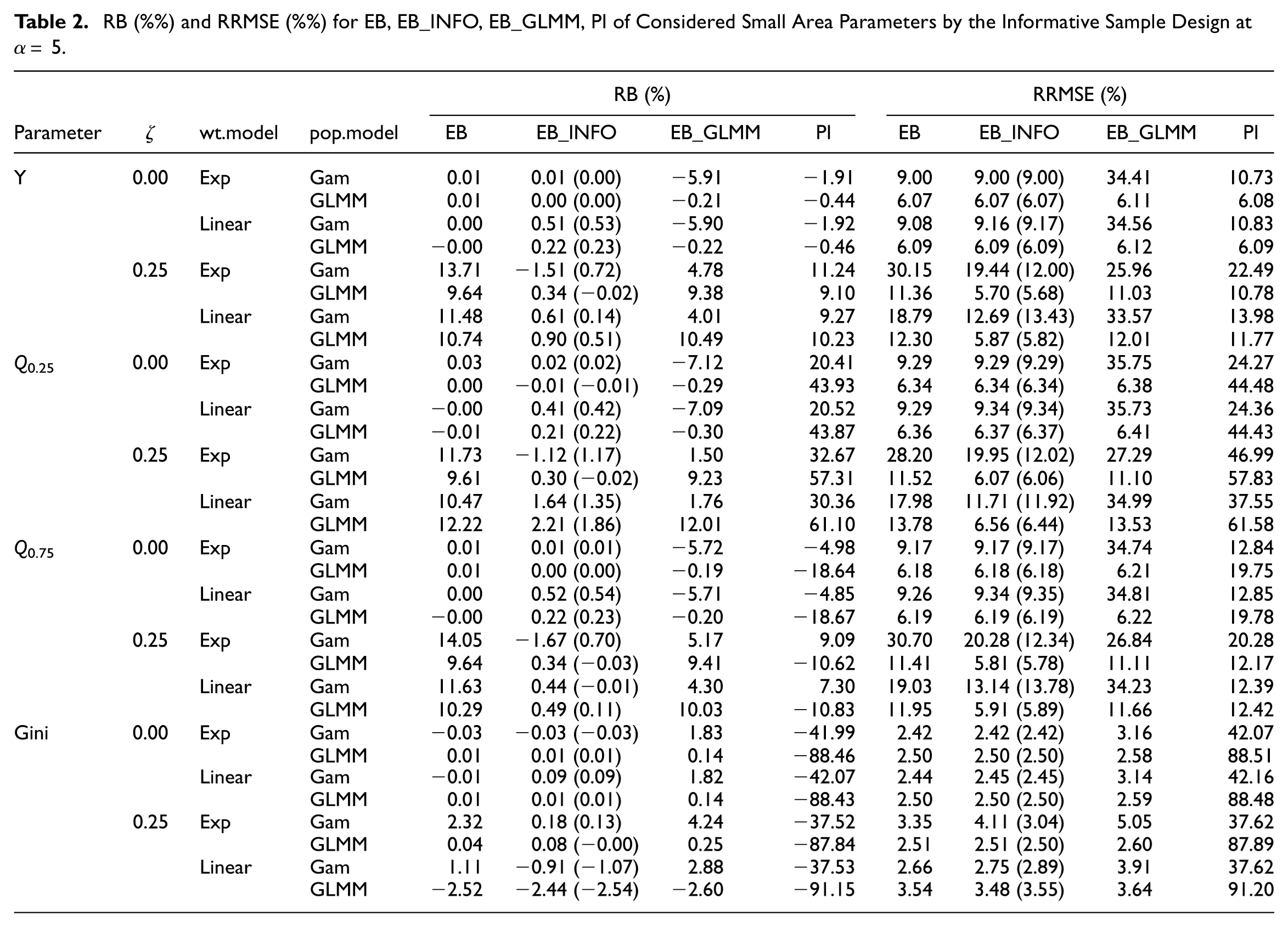
The averages of RB and RRMSE (in %) for areas are shown in Tables 1 and 2 for α= 2.5 and 5, respectively. Under noninformative sampling (ζ= 0), EB remains competitive with the alternatives, even when the population and inclusion probability models are misspecified. EB has the RB closest to zero in all scenarios and the RRMSE is smallest at both α= 2.5 and 5. EB_GLMM is robust to the linear inclusion probability model, but not when the population model is generated under the gamma-gamma model, as RB exceeds 5% when α= 5, and the RRMSE is much larger compared to EB or EB_INFO. Conversely, EB_INFO performs similarly to EB, with the RB of EB_INFO uniformly below 1% in absolute value and the RRMSE lower than that of EB_GLMM when the population model is misspecified. Under informative sampling (
RB (%) and RRMSE (%) for EB, EB_INFO, EB_GLMM, PI of Considered Small Area Parameters by the Informative Sample Design at α= 2.5.
RB (%) and RRMSE (%) for EB, EB_INFO, EB_GLMM, PI of Considered Small Area Parameters by the Informative Sample Design at α= 5.
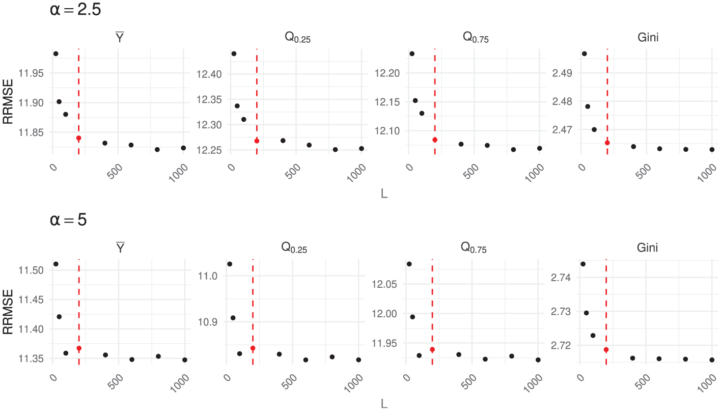
RRMSE (%) of EB_INFO under the gamma-gamma population model with an exponential inclusion probability, as L ranges from 25 to 1,000.
5.2. Simulation 2: Comparison of MSE Estimators
In Simulation 1, we observed that EB performs well even when the model is misspecified under noninformative sampling. Therefore, we focus on the performance of the MSE estimators in the scenario where the simulation data are generated from the gamma-gamma model with
We evaluate the MSE estimators described in Section 3 on the basis of two criteria. The first is a measure of the relative bias of the MSE estimator as a measure of the unconditional MSE of the predictor. This is defined as

where

and
where

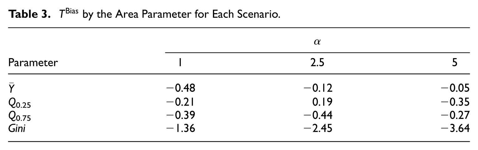
Several of the MSE estimators described in Section 3 include adjustments to correct for the bias in the estimation of the leading term. We therefore check whether there exists a bias for the leading term estimators. For this, define a test-statistic as
where
Figure 2 displays the relative biases of the alternative MSE estimators. The single-bootstrap MSE estimator (S) has a positive bias for
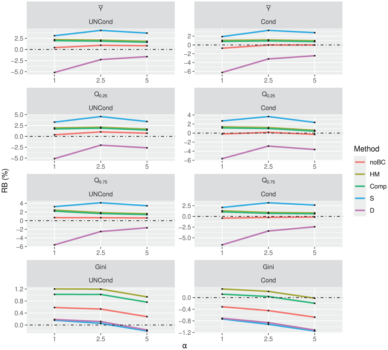
RB (%) of MSE estimators.
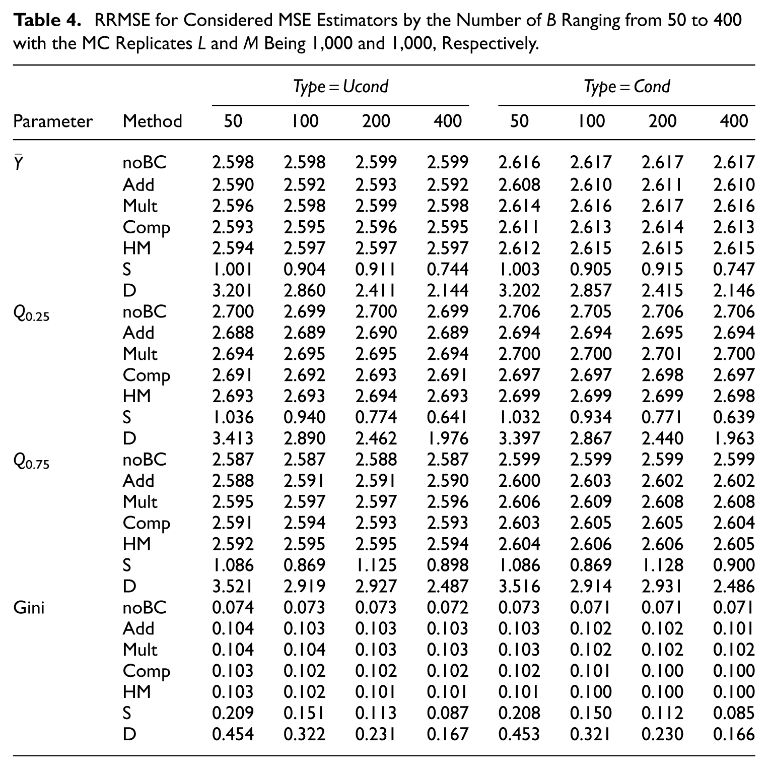
We performed a sensitivity analysis to determine the optimal number of bootstrap replications B, focusing on the first-round replications (B1) for methods S and D, while fixing B 2 = 1. The relative root mean square error (RRMSE) was used to evaluate the variability of MSE estimators, calculated similarly to Section 5.1. For completeness, the RRMSE of an MSE estimator with respect to the true MSE is defined as
where
Although Table 4 shows that the RRMSE for methods S and D decreases slightly as B increases, the magnitude of this change is minimal in our simulation setting because the second MSE component contributes very little relative to the leading term. As a result, increasing B beyond 100 yields only negligible improvement in the overall RRMSE while substantially increasing the computational burden. For this reason, and given the dominance of the leading term in our design, we set B= 100 for the simulation study, noting that users may perform their own sensitivity analyses when applying the method in practice.
RRMSE for Considered MSE Estimators by the Number of B Ranging from 50 to 400 with the MC Replicates L and M Being 1,000 and 1,000, Respectively.
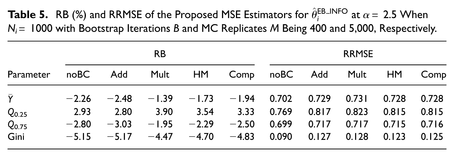
RB (%) and RRMSE of the Proposed MSE Estimators for
6. Application to Iowa Soil Erosion Data
We demonstrate the utility of the methods for estimating functions of sheet and rill erosion in Iowa counties. Sheet and rill erosion quantifies the soil loss due to the flow of water. Estimates of sheet and rill erosion for local areas are important for policy and planning purposes. Small area estimation for erosion is challenging because the erosion values have skewed distributions and are often available only from complex surveys.
The survey data for our study are from the National Resources Inventory (NRI). This longitudinal survey collects numerous variables related to agriculture and natural resources. We refer the reader to Nusser and Goebel (1997) and Berg and Kim (2021) for descriptions of the design of the NRI. Sheet and rill erosion is one of the primary response variables in the NRI. Estimates of sheet and rill erosion at the state level are produced as part of the standard NRI estimation program. County level estimation is generally considered a small area estimation problem in the NRI.
The auxiliary data are derived from the Cropland Data Layer (CDL). This raster layer provides a land cover classification for every cell on a grid covering the entire United States. We use the indicator that the CDL classification is corn as the covariate. This covariate is selected because crop managements are known to impact sheet and rill erosion.
Let y
ij
represent the soil erosion scaled by the sample standard deviation and x
ij
denote the indicator for the cornfield at the j-th sampled unit in the i-th county in Iowa. Note that all ninety-nine counties in Iowa were sampled. Across the ninety-nine counties in Iowa, the average number of potential sampling units per county (denoted N
i
) is approximately 363,778, ranging from 255,679 to 623,454. Among these, an average of 189 sampled units per county (denoted n
i
) were selected in the sample, with the number of sampled units ranging from 119 to 538. The resulting sampling proportion (
We fitted three models to the sampled data: the gamma-gamma model (Equation (2)), the generalized linear mixed model (GLMM; Equation (8)), and a linear mixed model (LMM) where y
ij
was transformed using a Box-Cox power transformation with a lambda parameter of 0.17. Note that we have implemented a grid search to determine the optimal λ under the REML framework, using the full linear mixed model as described in Rojas-Perilla et al. (2020). To evaluate their predictive performance, we conducted repeated random subsampling cross-validation. Specifically, in each of M= 100 iterations, the data were randomly split into 90% training and 10% testing sets. The models were trained on the training data, and predictions were generated for the test set. We calculated the mean squared error (MSE) between the predicted and actual values for each model in each iteration. The average MSEs over the 100 iterations were as follows: The gamma-gamma models, using the procedure described in Section 4 and the alternative procedure in Remark 2 of Section 4, achieved MSEs of 0.4370 and 0.4350, respectively. The GLMM yielded an MSE of 1.6622, while the LMM resulted in an MSE of 0.5592. These results indicate that the gamma-gamma model provided the best predictive performance among the models considered. Therefore, it was selected as the preferred model for the sample data in our analysis, with the estimates of the model parameters being
Figure 3 shows the predicted values of the following county-level parameters: the mean
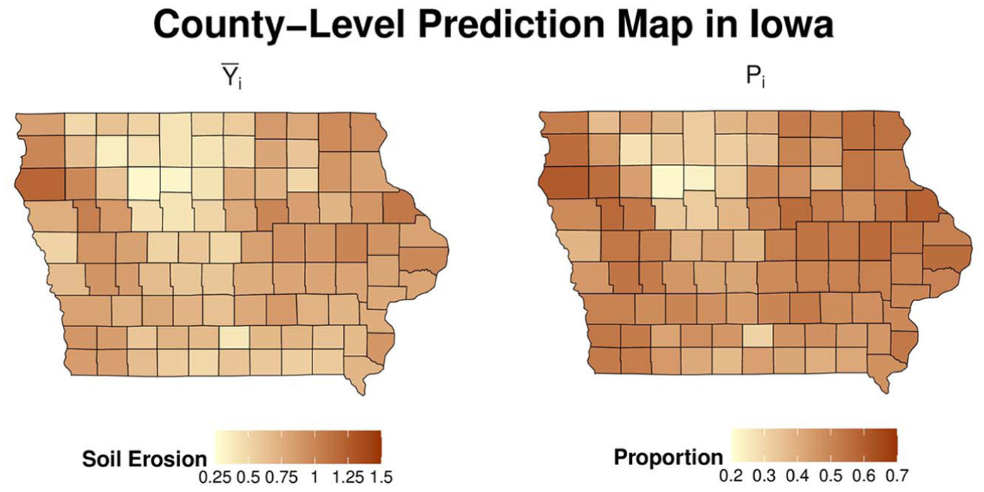
Prediction of the considered small area parameters with EB_INFO predictor.
We validate our analysis by comparing the direct estimator and the predicted values obtained under the gamma-gamma model without accounting for informative sampling (EB). (The direct estimators are computed using the survey::svydesign function in R.) As shown in Figure 4, the predicted values under informative sampling (EB_INFO) exhibit smaller absolute difference from the direct estimator than those under noninformative sampling, particularly in areas with larger sample sizes, for both small area parameters. Furthermore, as given in Figure 5, although both the direct estimator and EB_INFO exhibit reasonable coefficients of variation (CVs) within 20%, EB_INFO achieves smaller CVs for the nonlinear parameter (P m ) and demonstrates greater stability with fewer outliers.
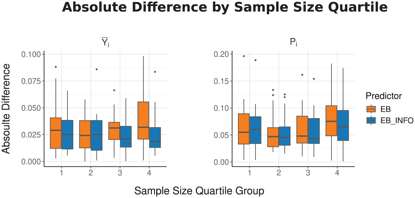
Absolute difference from the direct estimator by sample size quartile group for informative and noninformative predictors across two small area parameters.
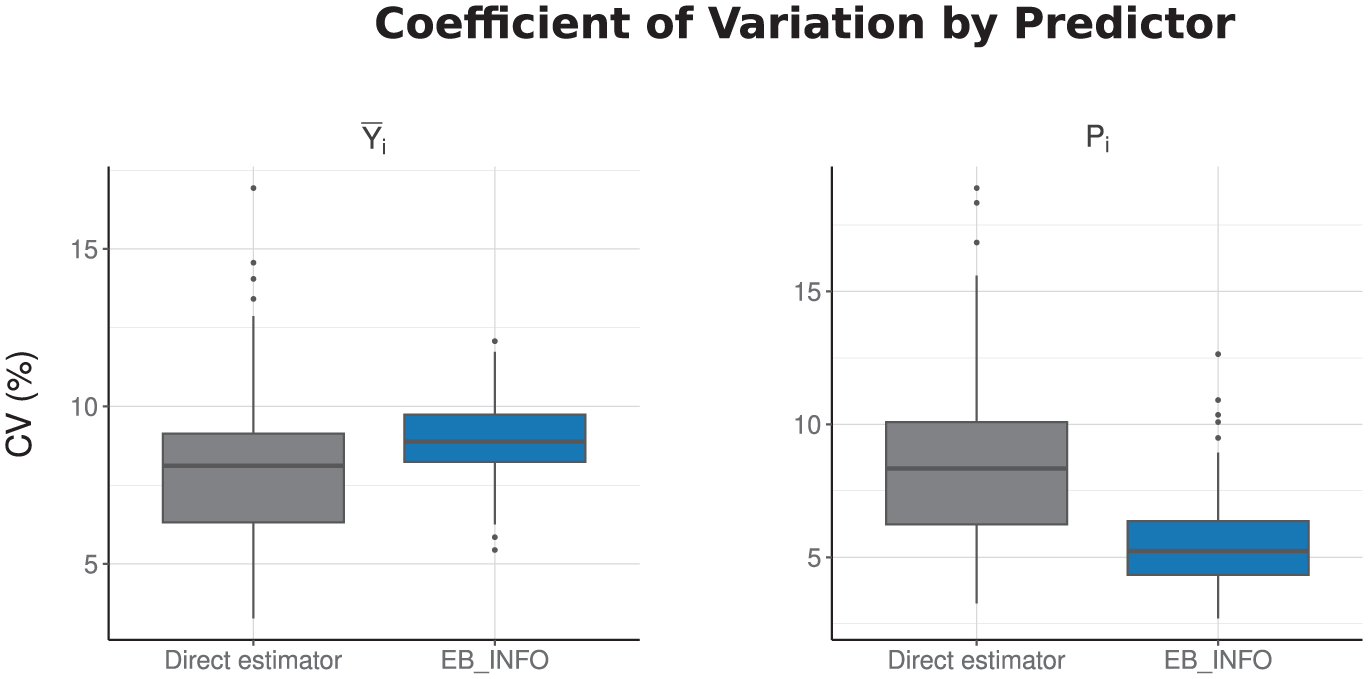
Comparison of the percent coefficient of variation (CV) between the direct estimator and the informative EB predictor for each small area parameter. We use
7. Conclusion
In this study, we have made several substantial contributions to the literature on small area estimation (SAE) under informative sampling designs. By performing extensive simulations, we have rigorously compared predictors under the gamma-gamma model with those derived under the gamma generalized linear mixed model (GLMM). Through sixteen distinct scenarios, we explored various levels of deviation from the underlying assumptions for the response variable y and sampling weight models, degrees of skewness in the response variable, and whether the sample design is informative. These simulations underscore the robustness of our gamma-gamma-based predictors and offer fresh insights into their relative performance across complex, realistic conditions.
Specifically, our results support the gamma-gamma model more than the gamma GLMM when dealing with skewed responses and informative designs. Additionally, we evaluated multiple MSE estimators for the gamma-gamma model, including one not previously paired with this framework. All relevant codes for the simulation study have been made publicly available to ensure reproducibility. The codes can be accessed at https://github.com/yhcho11/Gamma-Gamma-Informative/tree/main. Furthermore, we present a hierarchical formulation of the gamma-gamma model that simplifies the computational burden associated with marginal distributions used in earlier work. We also generalize the procedures of Hobza et al. (2020) to predict general small area parameters—a broader class of parameters than additive small area parameters, increasing the applicability and flexibility of our approach.
Despite these advancements, our work relies on the assumption that the covariates x ij are known for all elements of the population. While this condition is satisfied if covariates are sourced from a comprehensive census or administrative database, we acknowledge that it may be restrictive in some settings.
Building on our findings that the gamma distribution provides a robust framework for constructing small area predictors under skewed response variables, we plan to extend our approach to more complex sampling frameworks, including two-stage informative designs that consider non-sampled areas. Considering incomplete auxiliary information is another potential future research direction. Such endeavors will further broaden the applicability, robustness, and practical relevance of our gamma-gamma model–based SAE methods.
Supplemental Material
sj-pdf-1-jof-10.1177_0282423X261424813 – Supplemental material for Comparison of Small Area Procedures Based on Gamma Distributions with Extension to Informative Sampling
Supplemental material, sj-pdf-1-jof-10.1177_0282423X261424813 for Comparison of Small Area Procedures Based on Gamma Distributions with Extension to Informative Sampling by Yanghyeon Cho and Emily Berg in Journal of Official Statistics
Footnotes
Acknowledgements
We sincerely appreciate the valuable feedback from the Associate Editor and three anonymous reviewers.
Funding
The authors disclosed receipt of the following financial support for the research, authorship, and/or publication of this article: This work was partially supported by the U.S. Department of Agriculture’s National Resources Inventory, Cooperative Agreement NR203A750023C006, Great Rivers CESU 68-3A75-18-504.
Supplemental Material
Supplemental material for this article is available online.
Received: March 15, 2024
Accepted: January 20, 2026
References
Supplementary Material
Please find the following supplemental material available below.
For Open Access articles published under a Creative Commons License, all supplemental material carries the same license as the article it is associated with.
For non-Open Access articles published, all supplemental material carries a non-exclusive license, and permission requests for re-use of supplemental material or any part of supplemental material shall be sent directly to the copyright owner as specified in the copyright notice associated with the article.