How Does Noise Protection Affect the Accuracy of Life Expectancy and Other Demographic Indicators?

Abstract

New and efficient methods based on noise addition to protect the confidentiality in population statistics have been developed, tested, and applied in census production by various members of the European Statistical System over the past years. Basic demographic statistics—such as population stocks, live births and deaths by age, sex, and region—may be protected in a similar way, but also form the raw input to calculate various demographic indicators. This paper analyzes the impact on the accuracy of some selected indicators, namely fertility and mortality rates and life expectancies, under the assumption that the raw input counts are protected with a generic noise method with fixed variance parameter, by comparing the size of noise uncertainties with intrinsic statistical uncertainties using a Poisson model. As a by-product, we derive and validate numerically a closed analytical expression for the variance of life expectancies in a certain class of calculation models as a function of the variance of input mortality data. This expression also allows to calculate analytically the statistical uncertainty of life expectancies using the mentioned Poisson model for the input death counts.

1. Introduction

After the 2011 EU census, European Statistical System (ESS—the joint body of Eurostat and the national statistical institutes of all EU countries and Iceland, Liechtenstein, Norway, and Switzerland) experts realized that traditional statistical disclosure control (SDC) methods like cell suppression become inefficient when applied to very detailed cross-tabulations. Moreover, these methods do not protect outputs effectively when disseminated on non-nested geographical breakdowns like administrative regions and grids (geographic differencing); see Antal et al. (2017). Mainly for these two reasons, ESS efforts began from 2015 onwards to explore new SDC methods that avoid excessive information loss and also protect against geographic differencing. As a result, two methods based on adding some noise to the statistics were tested and recommended for the 2021 EU census (Antal et al. 2017; De Wolf et al. 2019a, 2019b), namely targeted record swapping (TRS; Frend et al. 2012) and the cell key method (CKM; Fraser and Wooton 2005; Marley and Leaver 2011; Thompson et al. 2013). A significant number of ESS members eventually decided to use one or a combination of these methods for their census outputs.

In the wake of the modernization of social statistics in the ESS, it is likely that also the annual demographic statistics would become more detailed and eventually integrated with multi-annual population statistics like censuses. This would entail some new questions, for example, whether some of these annual demographic statistics would require confidentiality protection; how the consistency with census-like (protected) statistics would be ensured; and finally how the key use cases of demographic statistics can be sufficiently ensured; cf. Schulte Nordholt et al. (2024).

For instance, basic demographic statistics including population stocks, live births and deaths by age, sex, and region are needed to calculate various demographic indicators at regional level. If the protection methods originally developed for census outputs were to be applied to these demographic statistics, the question arises how the additional noise-induced uncertainty propagates to the resulting indicator values. This paper analyzes the effects of a generic noise protection method with a fixed variance parameter on some selected demographic indicators. R code implementing the functions introduced in the paper is available on GitHub (https://github.com/bachfab/noisy_demo_indicators).

2. Noise Setup and Uncertainty Propagation

It is one of the features of the CKM introduced in Section 1 that the variance of the noise added to the output counts is a fixed input parameter, here denoted $V$ . Moreover, the detailed noise distributions of the CKM typically follow a discretized bell curve (as all noise terms must be integers to retain integer outputs) that is very close to a Gaussian (Bach 2021; Gießing 2016). Through these properties, the CKM is considered a reference example for a generic noise protection method in the sense mentioned above. (Note that TRS—the other method mentioned in Section 1—does not provide the same parametric control over the noise variance and therefore does not allow for such analytical studies of its effects.)

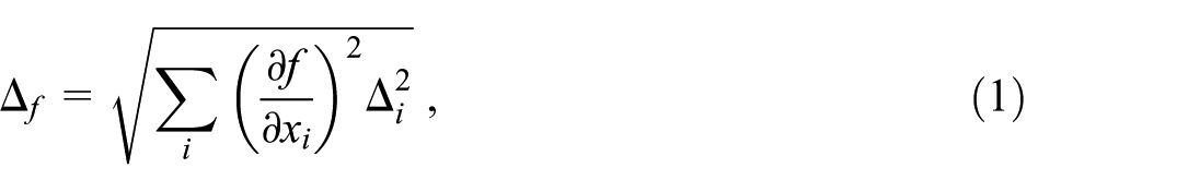
Furthermore, the standard theory of error propagation based on linear response of a measurement function $f\left(\mathbf{x}\right)$ to a set of uncorrelated input measurements $\mathbf{x}$ can be applied (for a recent reference textbook, see e.g., Morrison 2021):

$${\mathrm{\Delta }}_f=\sqrt{\sum _i{\left(\frac{\partial f}{\partial x_i}\right)}^2{\mathrm{\Delta }}_i^2},$$

(1)

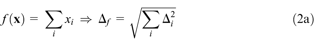
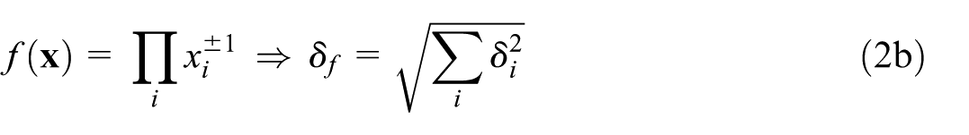
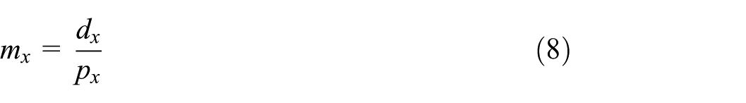
where $i$ runs over the elements of $\mathbf{x}$ with standard deviation ${\mathrm{\Delta }}_i\equiv \sqrt{\mathrm{Var}\left(x_i\right)}$ . From Equation (1) it is straightforward to derive two simple but handy special cases: when $f$ is a simple sum of independent input measurements, the squares of the absolute uncertainties are added; and when $f$ is a simple product (or ratio) of independent input measurements, the squares of relative uncertainties are added—that is,

$$f\left(\mathbf{x}\right)=\sum _i{x}_i\Rightarrow {\mathrm{\Delta }}_f=\sqrt{\sum _i{\mathrm{\Delta }}_i^2}$$

(2a)

$$f\left(\mathbf{x}\right)=\underset{i}{\Pi }{x}_i^{\pm 1}\Rightarrow {\delta }_f=\sqrt{\sum _i{\delta }_i^2}$$

(2b)

with relative uncertainties of the input measurements denoted ${\delta }_i={\mathrm{\Delta }}_i/x_i$ .

As a further simplification, in the specific setup analyzed here where only the CKM effect is to be considered, the standard deviation of all the input measurements $x_i$ is constant:

$${\mathrm{\Delta }}_i\equiv \mathrm{\Delta }=\sqrt{V}\forall i.$$

(3)

3. Results for Selected Demographic Indicators

For the quantitative analysis we select three demographic indicators that are generally very important for all kinds of demographic analysis: crude fertility and death rates, and life expectancy. On the rate indicators, that is, simple ratios of input counts, note various earlier studies such as Santos-Lozada et al. (2020), Hauer and Santos-Lozada (2021), and Bach (2021; see Section 4.3 thereof) that the present analysis expands on.

The three indicators depend on three distinct sets of raw input counts for a given region and time period: population stocks by sex and single years of age at the beginning and at the end of a given time period (typically a calendar year), as well as the number of live births (by mother’s single year of age) and the number of deaths (by sex and single year of age) during the same time period. To add some geographical granularity, we analyze all NUTS 2 regions of all ESS members for the latest available reference year 2023, as published in the data sets demo_r_d2jan (Eurostat 2025d), demo_r_fagec (Eurostat 2025c), and demo_r_magec (Eurostat 2025a).

3.1. Fertility Rates

The age-specific crude fertility rate is defined as

$$f_x=\frac{b_x}{w_x}$$

(4)

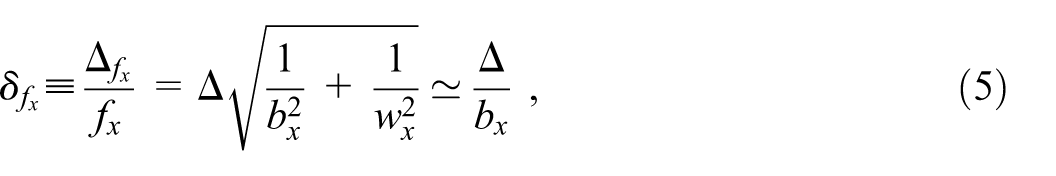
with $x$ the relevant age in single years, $b_x$ the number of live births by mothers aged $x$ and $w_x$ the average female population stock aged $x$ during the reference time period. Then the relative error on $f_x$ is given by Equation (2b) as

$${\delta }_{f_x}\equiv \frac{{\mathrm{\Delta }}_{f_x}}{f_x}=\mathrm{\Delta }\sqrt{\frac{1}{b_x^2}+\frac{1}{w_x^2}}\simeq \frac{\mathrm{\Delta }}{b_x},$$

(5)

where in the last step we neglect for simplicity a possible CKM uncertainty on $w_x$ , because $b_x<<w_x$ in general. In this approximation, the absolute uncertainty on $f_x$ from Equation (5) is ${\mathrm{\Delta }}_{f_x}=f_x{\delta }_{f_x}\simeq \mathrm{\Delta }/w_x$ .

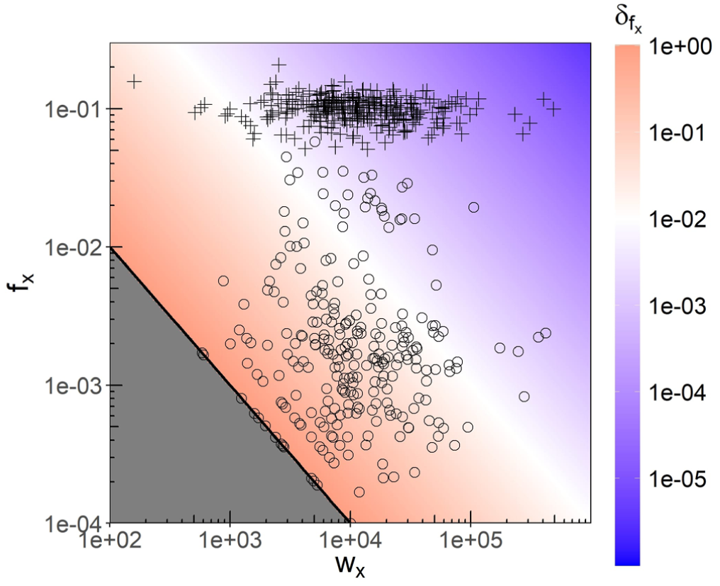
Setting $V=1$ and plugging in the numbers from the data sets, one finds that in the majority of cases the relative CKM uncertainty on the age-specific fertility rates is moderate, with a median relative uncertainty of $0.37\mathrm{\%}$ and more than $88\mathrm{\%}$ of all relative uncertainties ( $10854$ of $12287$ calculated) $<10\mathrm{\%}$ . Nevertheless, $33\mathrm{\%}$ of the uncertainties found ( $4061$ of $12287$ ) are $>1\mathrm{\%}$ . In line with Equation (5), as expected the largest relative uncertainties, up to $100\mathrm{\%}$ for $V=1$ , are found where the numbers of live births are very small, that is, $b_x<10$ down to $b_x=1$ . This is illustrated in Figure 1 showing the parametric plot of Equation (5) over the entire relevant $w_x$ – $f_x$ plane.

Figure 1.

Relative uncertainty on the age-specific fertility rate ${\delta }_{f_x}$ from CKM noise with variance $V=1$ as a function of the age-specific number of mothers $w_x$ and fertility rate $f_x$ according to Equation (5). The black line indicates the limiting contour corresponding to the number of live births $b_x=w_x{f}_x=1$ . Actual fertility rates found in the 2023 NUTS 2 data are shown for ages $x=16$ (circles) and $x=30$ (cross-hairs), showing that most ${\delta }_{f_{16}}>1\mathrm{\%}$ up to $100\mathrm{\%}$ while most ${\delta }_{f_{30}}<1\mathrm{\%}$ .

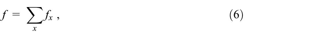
In addition to age-specific rates, one can also analyze the total fertility rate given as

$$f=\sum _x{f}_x,$$

(6)

so that by applying Equation (2a) and reusing ${\mathrm{\Delta }}_{f_x}$ , the relative uncertainty on $f$ amounts to

$${\delta }_f=\frac{{\mathrm{\Delta }}_f}{f}\simeq \frac{\mathrm{\Delta }}{f}\sqrt{\sum _x\frac{1}{w_x^2}}.$$

(7)

After plugging in the numbers, there is again little surprise that in this more aggregate indicator the CKM uncertainty is negligible in basically all cases calculated: more than $83\mathrm{\%}$ of all ${\delta }_f$ calculated ( $294$ of $356$ ) are $<0.1\mathrm{\%}$ , and ${\delta }_f>1\mathrm{\%}$ only for the smallest NUTS 2 region in the entire EU: Åland (FI20). Moreover, where input counts $b_x$ and $w_x$ are available for age bands, for example, $x\in \{20,\dots ,24\}$ , that have been protected with independent noise of the same variance $V$ as their single-year components (as the CKM does), the corresponding band-specific rates and total rate calculated from such age bands will be even less noisy. This is clear from Equations (5) and (7), where $b_x$ and $w_x$ only appear in the denominators. Finally, note that this section has not analyzed any bias resulting from noise addition: Enderle et al. (2018) show that such rates, that is, simple ratios, are approximately unbiased for sufficiently large denominators, more specifically that the ratio bias is already $<0.03$ for denominators $>10$ with noise setup $V=1$ and $D=3$ (which reflects well the noise scenario discussed here). This is generally valid for the purposes of this section and the next, where denominators are always $>100$ , except only average population used in Subsection 3.2 for a few terminal ages $>85$  years in Åland.

3.2. Mortality Rates

The age-specific crude mortality rate is defined as

$$m_x=\frac{d_x}{p_x}$$

(8)

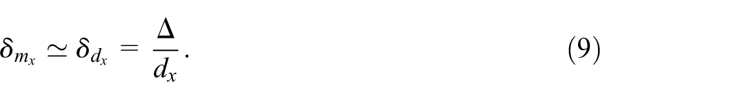
with $d_x$ the number of deaths at age $x$ and $p_x$ the average population during the reference time period. These rates can be calculated for the total population and for the male and female populations, respectively. Analogously to Equation (5) with $d_x<<p_x$ , the relative uncertainty is then

$${\delta }_{m_x}\simeq {\delta }_{d_x}=\frac{\mathrm{\Delta }}{d_x}.$$

(9)

Unlike for the fertility rates, the approximation $d_x<<p_x$ does not hold here in general for very high ages, but still holds up to the cut-off age 85 years applied in this analysis: the largest mortality rate found across the entire data set analyzed is $0.22$ —for males aged 85 years or over in Severozapaden (BG31)—and generally $<0.1$ for almost $99\mathrm{\%}$ of all rates calculated for all sex categories and regions.

Plugging in the NUTS 2 numbers from 2023 with $V=1$ , one finds qualitatively similar results to Subsection 3.1. However, quantitatively the median relative uncertainty is $1.4\mathrm{\%}$ for the total population across all ages ( $2.2\mathrm{\%}$ for male and $2.9\mathrm{\%}$ for female populations), and in the total population $23\mathrm{\%}$ of all uncertainties calculated are $>10\mathrm{\%}$ ( $27\mathrm{\%}$ respectively $33\mathrm{\%}$ for males and females). This is because the small-number effect already discussed in Subsection 3.1 is much more pronounced in the age-specific mortality rates: deaths are spread across all ages instead of just a fertile age band (e.g., 16–44 years), and they are (fortunately) very scarce across a majority of ages, increasing only in the terminal ages. Therefore, age-specific death rates stemming from very small death counts $d_x<10$ are much more numerous than age-specific fertility rates, especially at the NUTS 2 level considered here, leading to the larger typical relative uncertainties found above.

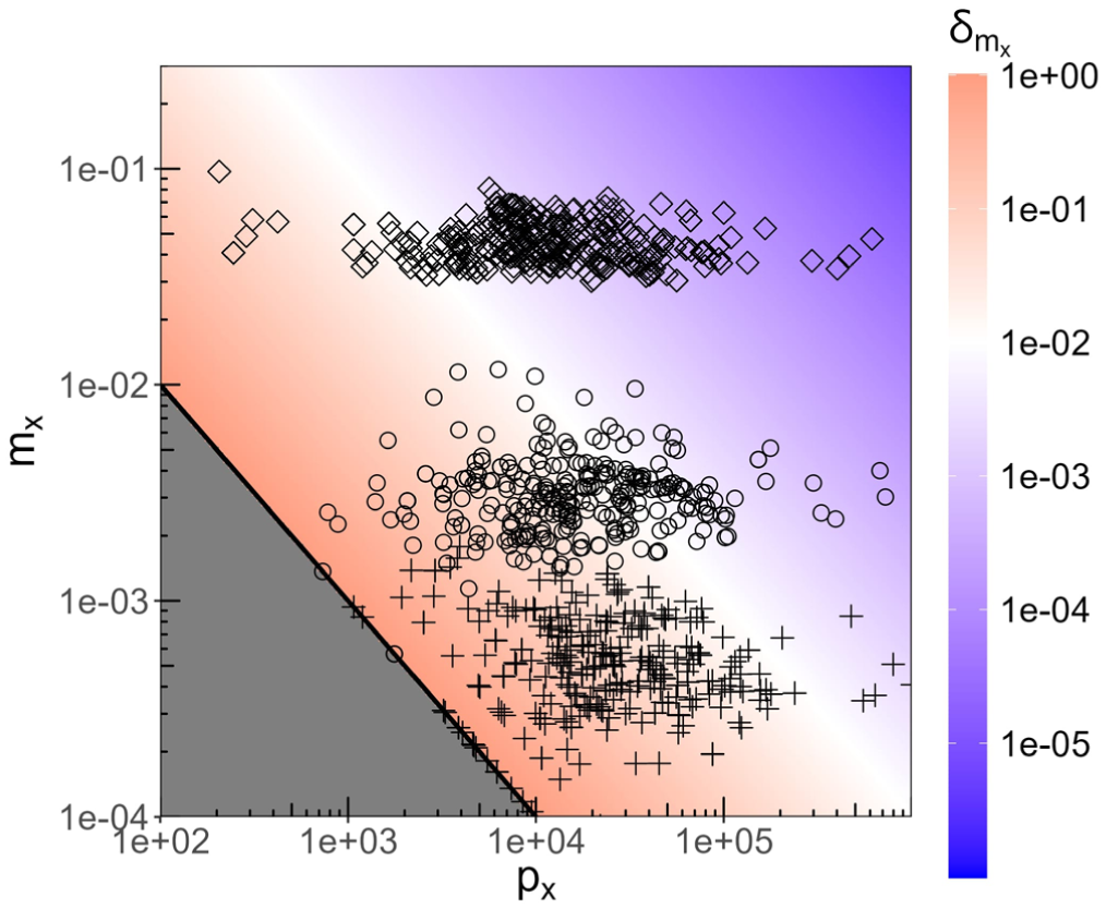
As for the fertility rates, Figure 2 shows the parametric dependence of ${\delta }_{m_x}(p_x,m_x)$ according to Equation (9) over the entire relevant parameter space and showing some actual data points from the 2023 NUTS 2 data. Moreover, as for the fertility rates, in noise protection methods where count aggregates receive independent noise, the rates for multi-year age bands will be more accurate than for single years; see discussion in Subsection 3.1.

Figure 2.

Relative uncertainty on the age-specific mortality rate ${\delta }_{m_x}$ from CKM noise with variance $V=1$ as a function of age-specific population $p_x$ and crude mortality rate $m_x$ according to Equation (9). The black line indicates the limiting contour corresponding to the number of deaths $d_x=p_x{m}_x=1$ . Actual crude mortality rates found in the 2023 NUTS 2 data are shown for ages $x=0$ (circles), $x=30$ (cross-hairs), and $x=80$ (diamonds), showing that most ${\delta }_{m_{0,30}}>1\mathrm{\%}$ up to $100\mathrm{\%}$ while most ${\delta }_{m_{80}}<1\mathrm{\%}$ .

3.3. Life Expectancy

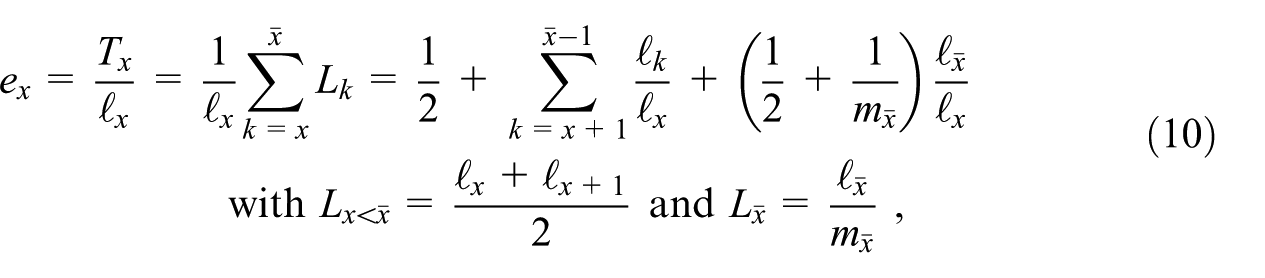
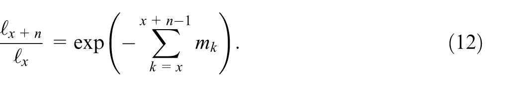
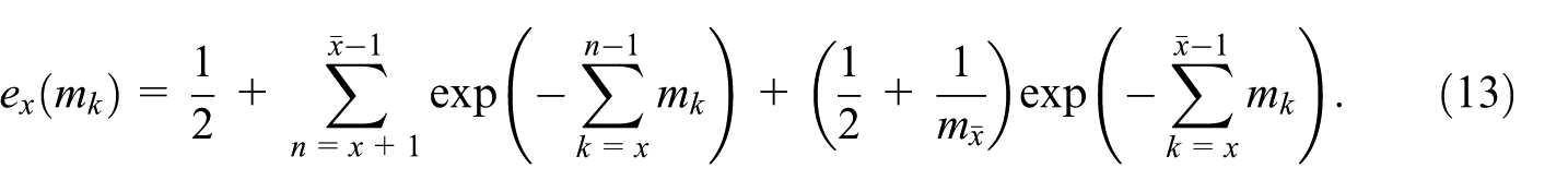
The calculation of age-specific life expectancy $e_x$ is considerably more complex than that of the crude rates presented in the previous sections. Therefore, also the uncertainty propagation according to Equation (1) is more complex and it is worthwhile to use the auxiliary indicators published in the so-called life table, see data set demo_r_mlife (Eurostat 2025b) for the ESS (note that the NUTS 2 regions of Germany are not available in the data set and therefore not analyzed here). Most notably, we make use of the total number of person-years lived from age $x$ until all have died ( $T_x$ ), the total number of person-years lived from age $x$ to $x+1$ ( $L_x$ ), the survivorship function ( ${\ell }_x$ ) and the age-specific mortality rate ( $m_x$ ), all included in the life table. The sole raw data input is through $m_x$ depending on the raw number of age-specific deaths $d_x$ and the average population of that age $p_x$ for the given period. All other life table indicators and ultimately $e_x$ are derived from this as follows (cf. e.g., Eurostat’s life expectancy methodology documented at https://ec.europa.eu/eurostat/cache/metadata/Annexes/demo_mor_esms_an_1.pdf):

$$\begin{array}{c}\multicolumn{1}{c}{e_x=\frac{T_x}{{\ell }_x}=\frac{1}{{\ell }_x}\sum _{k=x}^{\overline{x}}{L}_k=\frac{1}{2}+\sum _{k=x+1}^{\overline{x}-1}\frac{{\ell }_k}{{\ell }_x}+(\frac{1}{2}+\frac{1}{m_{\overline{x}}})\frac{{\ell }_{\overline{x}}}{{\ell }_x}}\\ \multicolumn{1}{c}{\mathrm{with}{L}_{x<\overline{x}}=\frac{{\ell }_x+{\ell }_{x+1}}{2}\mathrm{and}{L}_{\overline{x}}=\frac{{\ell }_{\overline{x}}}{m_{\overline{x}}},}\end{array}$$

(10)

where the sums run from the age $x$ in question until the open-ended terminal age class $\overline{x}$ where the age-specific tabulation stops. The cut-off age depends on national publication practices and other constraints; for example, in the EU life tables (Eurostat 2025b) this terminal age class was “85 years or over” at the time of writing this paper. Note the explicit dependency on the terminal mortality rate $m_{\overline{x}}$ entering through the terminal person-years lived $L_{\overline{x}}$ . In general, there is some freedom in modeling $L_{\overline{x}}$ as a function of $m_{\overline{x}}$ , where the relation above is the one used by Eurostat. A further implicit dependency on all other mortality rates $m_{x<\overline{x}}$ enters through the ${\ell }_x$ which are here defined recursively as

$${\ell }_{x+1}={\ell }_x\exp (-m_x)\mathrm{with}{\ell }_o\equiv 100000,$$

(11)

so that

$$\frac{{\ell }_{x+n}}{{\ell }_x}=\exp (-\sum _{k=x}^{x+n-1}{m}_k).$$

(12)

The attentive reader may have noted the difference between the definitions of the survivorship function in the Eurostat methodology and here in Equation (11): The two definitions have the same Taylor expansion in $m_x$ down to $\mathcal{O}\left(m_x^3\right)$ . Since prevalently $m_x<<1$ (cf. Subsection 3.2), the definitions are therefore equivalent for all practical purposes, while the exponential definition of Equation (11), used for example, in the U.S. (see https://www.lifeexpectancy.org/lifetable.shtml), allows for the following analytic manipulations necessary to derive Equation (16).

Equation (12) can be plugged into Equation (10) to replace all $\ell$ ratios, giving

$$e_x\left(m_k\right)=\frac{1}{2}+\sum _{n=x+1}^{\overline{x}-1}\exp (-\sum _{k=x}^{n-1}{m}_k)+(\frac{1}{2}+\frac{1}{m_{\overline{x}}})\exp (-\sum _{k=x}^{\overline{x}-1}{m}_k).$$

(13)

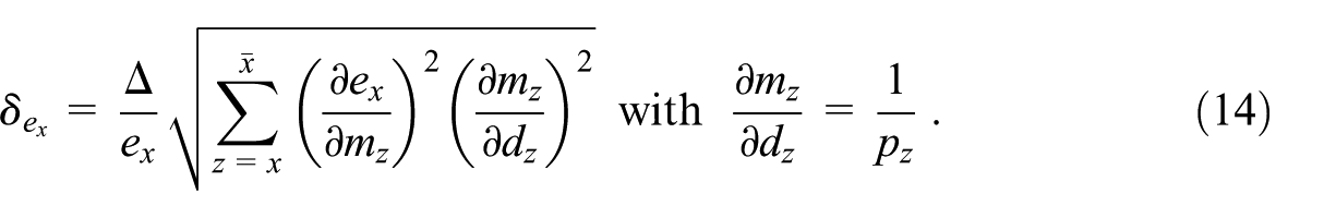
To derive the uncertainty on $e_x$ , one needs the functional dependency of $m_k$ on $d_k$ and $p_k$ . While again there is some methodological freedom in modeling the mortality rates for life expectancy purposes (e.g., the UK’s Office for National Statistics averages over the three most recent years, see https://www.ons.gov.uk/peoplepopulationandcommunity/healthandsocialcare/healthandlifeexpectancies/methodologies/guidetocalculatingnationallifetables), we assume here for practical purposes the simplest model—also used by Eurostat—that employs the crude age-specific mortality rate of Equation (8), that is, $m_k=d_k/p_k$ . Ignoring again any potential noise on $p_k$ , as argued in Subsection 3.1, Equation (13) can now be differentiated with respect to the raw input $d_k$ using the chain rule to calculate the resulting uncertainty on $e_x$ as

$${\delta }_{e_x}=\frac{\mathrm{\Delta }}{e_x}\sqrt{\sum _{z=x}^{\overline{x}}{\left(\frac{\partial e_x}{\partial m_z}\right)}^2{\left(\frac{\partial m_z}{\partial d_z}\right)}^2}\mathrm{with}\frac{\partial m_z}{\partial d_z}=\frac{1}{p_z}.$$

(14)

To evaluate the derivative term $(\partial e_x/\partial m_z)$ , consider rewriting the exponential of a sum as a product of exponentials, that is,

$$\exp \left(\sum _k{\alpha }_k\right)=\underset{k}{\Pi }{A}_k\mathrm{with}{A}_k=\exp \left({\alpha }_k\right),$$

and then consider a sum over such products of exponentials expanded as

$$A_1+A_1{A}_2+\dots +A_1{A}_2\cdots A_z+A_1{A}_2\cdots A_z{A}_{z+1}+\cdots .$$

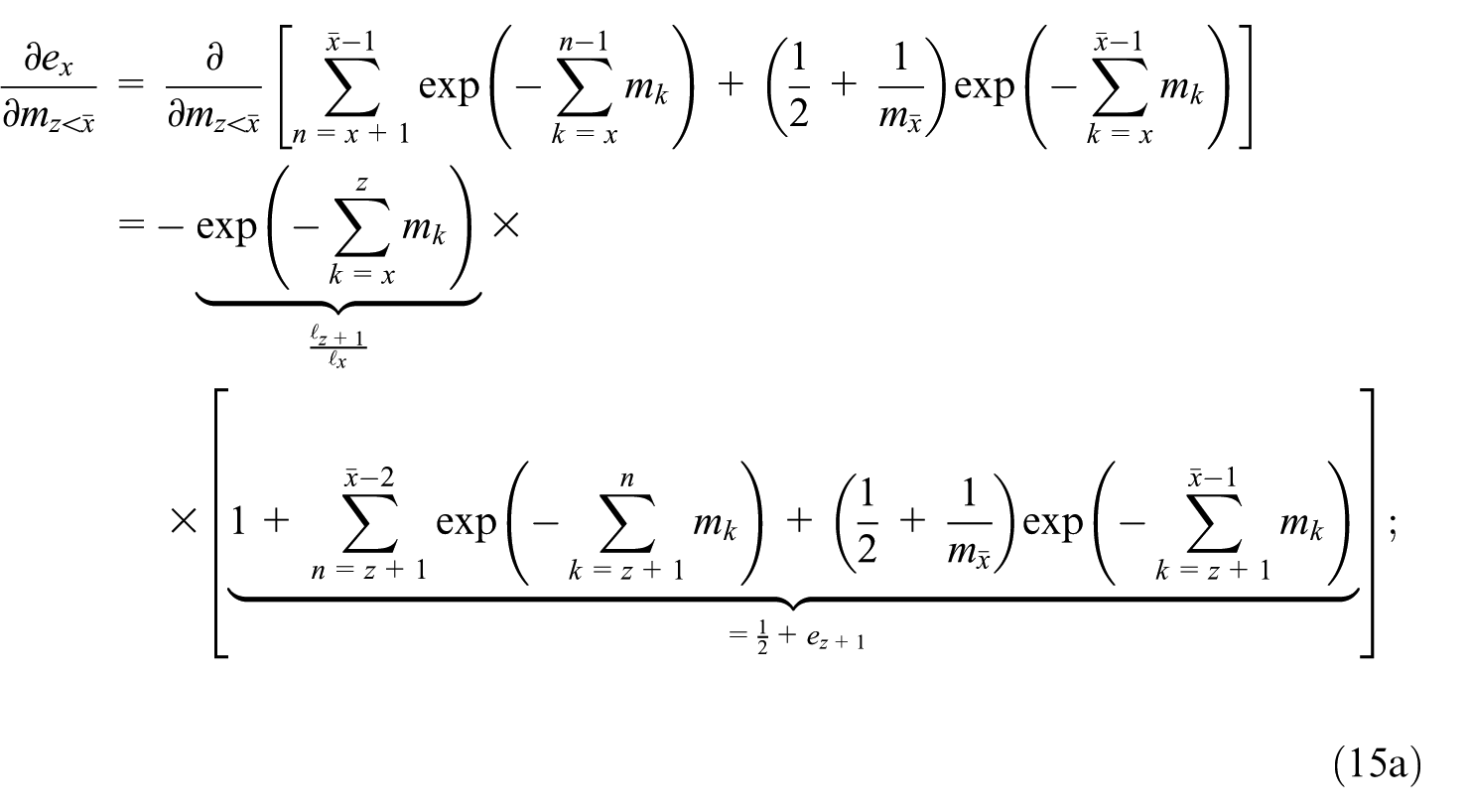
The derivative of this expression with respect to index $z$ has the form

$$(A_1{A}_2\cdots A_z)(1+A_{z+1}+\cdots ).$$

Applying this to the derivative term $(\partial e_x/\partial m_z)$ in Equation (14), with $e_x\left(m_z\right)$ from Equation (13), gives

$$\begin{array}{c}\multicolumn{1}{c}{\frac{\partial e_x}{\partial m_{z<\overline{x}}}=\frac{\partial }{\partial m_{z<\overline{x}}}[\sum _{n=x+1}^{\overline{x}-1}\exp (-\sum _{k=x}^{n-1}{m}_k)+(\frac{1}{2}+\frac{1}{m_{\overline{x}}})\exp (-\sum _{k=x}^{\overline{x}-1}{m}_k)]}\\ \multicolumn{1}{c}{=-\underset{\frac{{\ell }_{z+1}}{{\ell }_x}}{\underbrace{\exp (-\sum _{k=x}^z{m}_k)}}\times }\\ \multicolumn{1}{c}{\times \left[\underset{=\frac{1}{2}+e_{z+1}}{\underbrace{1+\sum _{n=z+1}^{\overline{x}-2}\exp (-\sum _{k=z+1}^n{m}_k)+(\frac{1}{2}+\frac{1}{m_{\overline{x}}})\exp (-\sum _{k=z+1}^{\overline{x}-1}{m}_k)}}\right];}\\ \multicolumn{1}{c}{}\end{array}$$

(15a)

$$\frac{\partial e_x}{\partial m_{\overline{x}}}=-\frac{1}{m_{\overline{x}}^2}\frac{{\ell }_{\overline{x}}}{{\ell }_x},$$

(15b)

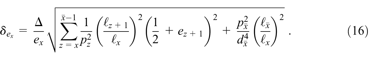
where Equations (12) and (13) were used in Equation (15a) to identify expressions in terms of ${\ell }_{z+1}$ and $e_{z+1}$ . This can be plugged back into Equation (14) to obtain the final formula for the relative uncertainty

$${\delta }_{e_x}=\frac{\mathrm{\Delta }}{e_x}\sqrt{\sum _{z=x}^{\overline{x}-1}\frac{1}{p_z^2}{\left(\frac{{\ell }_{z+1}}{{\ell }_x}\right)}^2{(\frac{1}{2}+e_{z+1})}^2+\frac{p_{\overline{x}}^2}{d_{\overline{x}}^4}{\left(\frac{{\ell }_{\overline{x}}}{{\ell }_x}\right)}^2}.$$

(16)

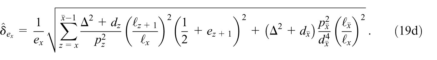
Since the analytical derivation of this result via Equations (13), (14), (15a), and (15b) is not straightforward, its correctness is validated numerically in Appendix A. Equation (16) represents a closed analytical expression for ${\delta }_{e_x}$ for a class of life expectancy calculation methods characterized by Equations (11) and (8), which includes the EU method. It allows the straightforward calculation of ${\delta }_{e_x}$ from the CKM setup (recall $\mathrm{\Delta }=\sqrt{V}$ ), from the life table indicators ${\ell }_x$ and $e_x$ , and from the population stocks $p_x$ and the terminal death number $d_{\overline{x}}$ .

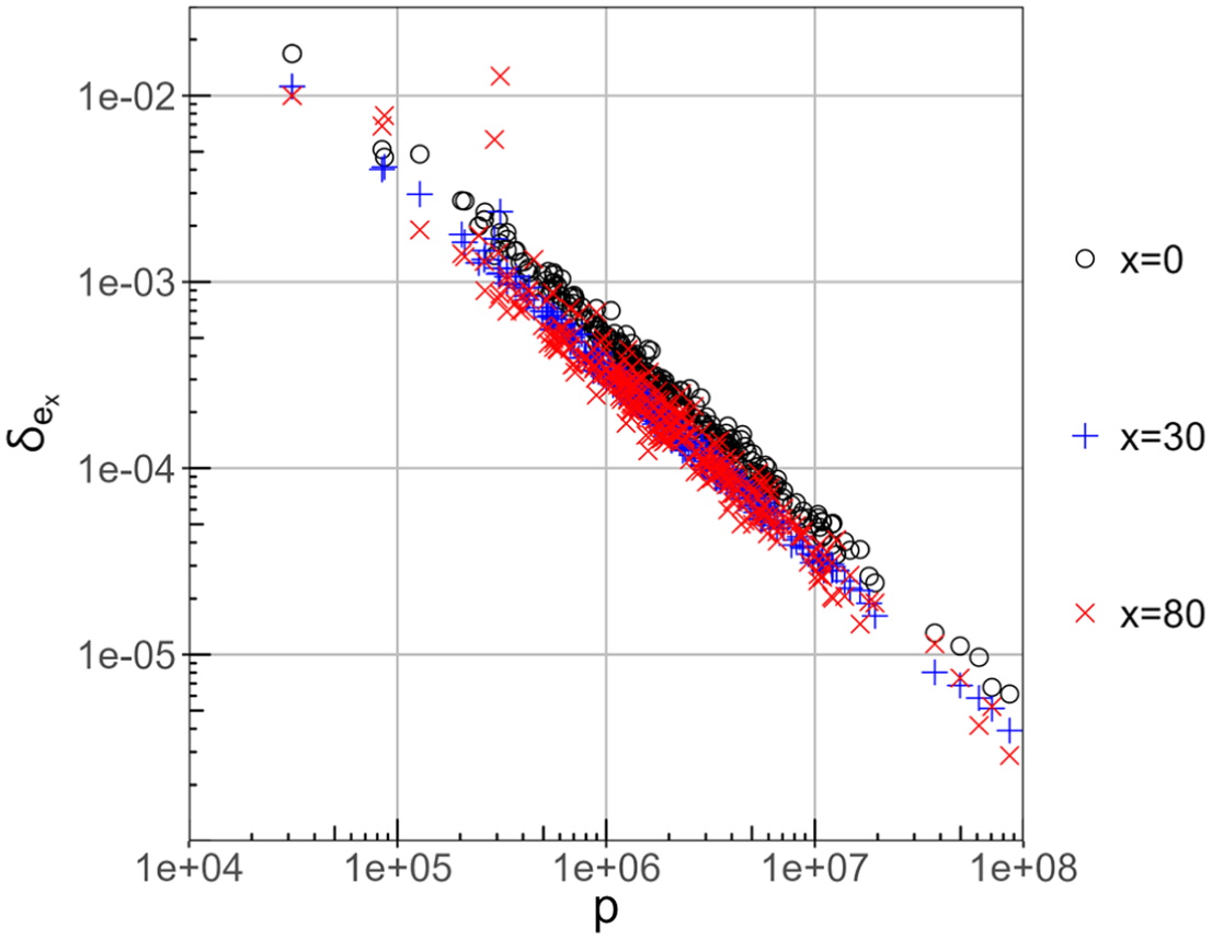
Plugging in the 2023 numbers for NUTS 2 regions published by Eurostat with $V=1$ , one finds very moderate relative uncertainties on the age-specific life expectancies largely prevailing, with a median ${\delta }_{e_x}=0.018\mathrm{\%}$ for the total population ( $0.037\mathrm{\%}$ for the male population and $0.035\mathrm{\%}$ for the female population), and ${\delta }_{e_x}>1\mathrm{\%}$ for the total population occurring only in two NUTS 2 regions: Mayotte (FRY5) and again the smallest one, Åland (FI20); see the corresponding data points in Figure 3 above the ${\delta }_{e_x}=1\mathrm{\%}$ line at total population values $p\simeq 3\times {10}^5$ (Mayotte) and $p\simeq 3\times {10}^4$ (Åland). Furthermore, Equation (16) suggests an inverse correlation ${\delta }_{e_x}~{\overline{p}}_x$ with the total (male or female) population aged $\ge x$ of a given region ${\overline{p}}_x=\sum _{k=x}^{\overline{x}}{p}_k$ (i.e., $p\equiv {\overline{p}}_0$ ). This is also illustrated in Figure 3 for various ages $x$ .

Figure 3.

Scatter plot of the relative uncertainty from CKM noise on the life expectancy ${\delta }_{e_x}$ at ages $x=0$ , 30, and 80, according to Equation (16), over the total population $p$ , with one dot for each ESS region analyzed.

4. Statistical Fluctuations

Section 3 dealt solely with the effects of artificially adding noise according to a given setup to the raw input counts. A full analysis of the performance of such protection methods, however, should compare these effects to the intrinsic statistical fluctuations that always affect these raw counts—and hence the resulting derived indicators—as well. To obtain a model for these statistical fluctuations, it is a widely used practice in the literature to consider vital events as rare events during the reference period and thus as Poisson distributed; cf. for example, Scott (1981) and Peters et al. (2009). Then the Poisson parameter $\lambda$ , and hence the variance stemming from statistical fluctuation, of any given event count $x_i$ can be estimated by the count itself: $\lambda =\mathrm{Var}\simeq x_i$ thus giving

$${\tilde{\mathrm{\Delta }}}_i=\sqrt{x_i},$$

(17)

where the tilde is to indicate that this uncertainty comes from intrinsic statistical variation (analog ${\tilde{\delta }}_i$ for relative uncertainties).

It can be verified with the data sets used in Section 3 that this provides a robust estimation of the size of the intrinsic statistical variation, namely by calculating the standard deviation across the entire available time series for each NUTS 2 region by age and sex, and dividing it by the estimator of Equation (17). In the death counts, the median of this ratio over all available regions and ages is 1.2 (with lower and upper quartiles $1.0-1.7$ ) for males and 1.1 (lower/upper quartiles $0.9-1.6$ ) for females. In the live birth counts, the median is 1.8 (lower/upper quartiles $1.2-3.2$ ). This shows that the variance estimator of Equation (17) indeed provides a robust estimate of the magnitude of the statistical variation. There is a systematic under-estimation of the actual variation over time (more so in the live births than in the deaths). However, this is not surprising because the validation approach assumes a constant Poisson parameter—that is, constant event rates—over the entire time series, which obviously underestimates the true variation. To reduce this sensitivity of the validation to demographic dynamics, we restrict the validation to infant mortality $d_0$ for the 100 NUTS 2 regions with the smallest total fertility variation. Infant mortality is relatively stable compared to fertility or older-age mortality, so demographic trends have less impact. By choosing regions with low fertility variation, we further minimize demographic changes that hamper the comparison. Here the median ratio of the standard deviation over its estimator for both sexes together is 1.1 (with lower and upper quartiles $1.0-1.4$ ).

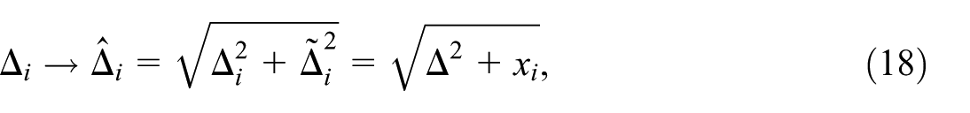
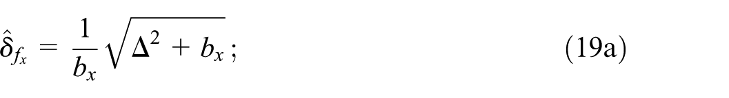
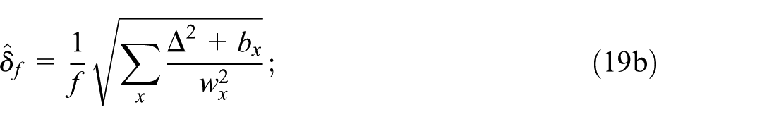
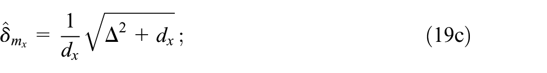
Using Equation (17), all uncertainties calculated in Section 3 can be modified or extended in a straightforward manner to reflect either statistical uncertainties or the combination of statistical and CKM noise uncertainties. In all cases, the new expressions for combined uncertainties (indicated by a hat) result from replacing

$${\mathrm{\Delta }}_i\to {\hat{\mathrm{\Delta }}}_i=\sqrt{{\mathrm{\Delta }}_i^2+{\tilde{\mathrm{\Delta }}}_i^2}=\sqrt{{\mathrm{\Delta }}^2+x_i},$$

(18)

For ease of reference, we write out the modified Equations (5), (7), (9), and (16):

$${\hat{\delta }}_{f_x}=\frac{1}{b_x}\sqrt{{\mathrm{\Delta }}^2+b_x};$$

(19a)

$${\hat{\delta }}_f=\frac{1}{f}\sqrt{\sum _x\frac{{\mathrm{\Delta }}^2+b_x}{w_x^2}};$$

(19b)

$${\hat{\delta }}_{m_x}=\frac{1}{d_x}\sqrt{{\mathrm{\Delta }}^2+d_x};$$

(19c)

$${\hat{\delta }}_{e_x}=\frac{1}{e_x}\sqrt{\sum _{z=x}^{\overline{x}-1}\frac{{\mathrm{\Delta }}^2+d_z}{p_z^2}{\left(\frac{{\ell }_{z+1}}{{\ell }_x}\right)}^2{(\frac{1}{2}+e_{z+1})}^2+({\mathrm{\Delta }}^2+d_{\overline{x}})\frac{p_{\overline{x}}^2}{d_{\overline{x}}^4}{\left(\frac{{\ell }_{\overline{x}}}{{\ell }_x}\right)}^2}.$$

(19d)

In all cases, setting $\mathrm{\Delta }=0$ produces a formula for the purely statistical uncertainty assuming the above-mentioned Poisson model.

5. Combined Analysis and NUTS 3 Picture

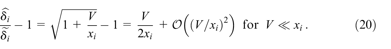
A full assessment of the effects of noisy SDC setups based on CKM or similar methods (the key property being a constant noise variance parameter) on the quality of demographic indicators must compare the total uncertainties ( ${\hat{\mathrm{\Delta }}}_i$ , ${\hat{\delta }}_i$ ) to a scenario of only statistical uncertainties ( ${\tilde{\mathrm{\Delta }}}_i$ , ${\tilde{\delta }}_i$ ), rather than comparing pure noise effects ( ${\mathrm{\Delta }}_i$ , ${\delta }_i$ ) to a scenario of no uncertainties at all. To this end, we make use of Equations (19a) to (19d) to analyze the relative contribution of CKM noise in the total uncertainty, calculated as ${\hat{\delta }}_i/{\tilde{\delta }}_i-1$ ( $={\hat{\mathrm{\Delta }}}_i/{\tilde{\mathrm{\Delta }}}_i-1$ ). For the age-specific crude rates $f_x$ and $m_x$ , Equations (19a) and (19c), there is a simple analytic expression as a function of the crude input event count that illustrates the limit in which the CKM contribution becomes negligible:

$$\frac{\widehat{{\delta }_i}}{\widetilde{{\delta }_i}}-1=\sqrt{1+\frac{V}{x_i}}-1=\frac{V}{2x_i}+\mathcal{O}\left({(V/x_i)}^2\right)\mathrm{for}V<<x_i.$$

(20)

This makes explicit that relative CKM noise effects for these rates are small and thus negligible except where the CKM variance parameter is of the same order of magnitude as the crude event count, that is, $x_i~\mathcal{O}\left(V\right)$ . However, since $V~\mathcal{O}\left(1\right)$ (e.g., $V\le 5$ ) by design in all practical scenarios, this implies a regime where the statistical fluctuations are large, too, since ${\tilde{\delta }}_i=1/\sqrt{x_i}~\mathcal{O}(1/\sqrt{V})~\mathcal{O}\left(1\right)$ .

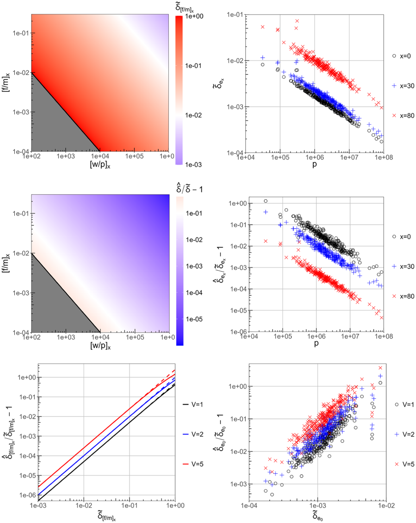
Figure 4 shows the comprehensive results for the age-specific fertility and mortality rates as well as for the life expectancies. These results illustrate several key insights:

• in general, statistical fluctuations ${\tilde{\delta }}_i$ (assuming the Poisson model of Section 4) are an important source of uncertainty for all indicators considered here, with relative uncertainties $>1\mathrm{\%}$ and up to $10\mathrm{\%}$ for life expectancies in the higher age bands for populations $<100000$ people, and up to $100\mathrm{\%}$ for age-specific event rates with underlying crude event counts of $\mathcal{O}\left(1\right)$ ;

• for the crude rates $f_x$ and $m_x$ , the relative contribution of CKM noise to the total uncertainty ${\hat{\delta }}_i$ remains negligible—that is, ${\hat{\delta }}_i/{\tilde{\delta }}_i-1<10\mathrm{\%}$ —everywhere except in the extreme corners of the parameter space where the statistical fluctuations themselves become large, ${\tilde{\delta }}_i~\mathcal{O}\left(1\right)$ , confirming the approximation of Equation (20);

• for the life expectancies $e_x$ , the relative contribution of CKM noise to the total uncertainty ${\hat{\delta }}_i$ is generally larger than for the crude rates, with ${\hat{\delta }}_i/{\tilde{\delta }}_i-1~\mathcal{O}\left(100\mathrm{\%}\right)$ for populations $<100000$ people and corresponding relative statistical fluctuations ${\tilde{\delta }}_i~\mathcal{O}\left(1\mathrm{\%}\right)$ ;

• while increasing the CKM variance parameter within a realistic range $V<~5$ has a notable effect on the relative CKM noise contribution to the total uncertainty ${\hat{\delta }}_i$ , even the $V=5$ scenario does not generally lead to a situation where the CKM contribution becomes dominant for any indicator ( ${\hat{\delta }}_i/{\tilde{\delta }}_i-1>300\mathrm{\%}$ only for life expectancy at birth $e_0$ of the smallest NUTS 2 region Åland with a population of $~30000$ people).

Figure 4.

Relative uncertainties from statistical fluctuations $\tilde{\delta }$ (top row) as well as relative contribution of CKM noise to the total uncertainty $\hat{\delta }/\tilde{\delta }-1$ against population size with CKM variance $V=1$ (center row) and against statistical uncertainty $\tilde{\delta }$ for various $V$ values (bottom row), as analytic plots for simple age-specific fertility rates $f_x$ resp. crude mortality rates $m_x$ (left column) and as scatter plots showing the 2023 NUTS 2 data for age-specific life expectancies $e_x$ (right column). All results based on Equations (19a)–(19d) and (20) (the linear approximation of Equation (20) is shown dashed in the bottom–left plot).

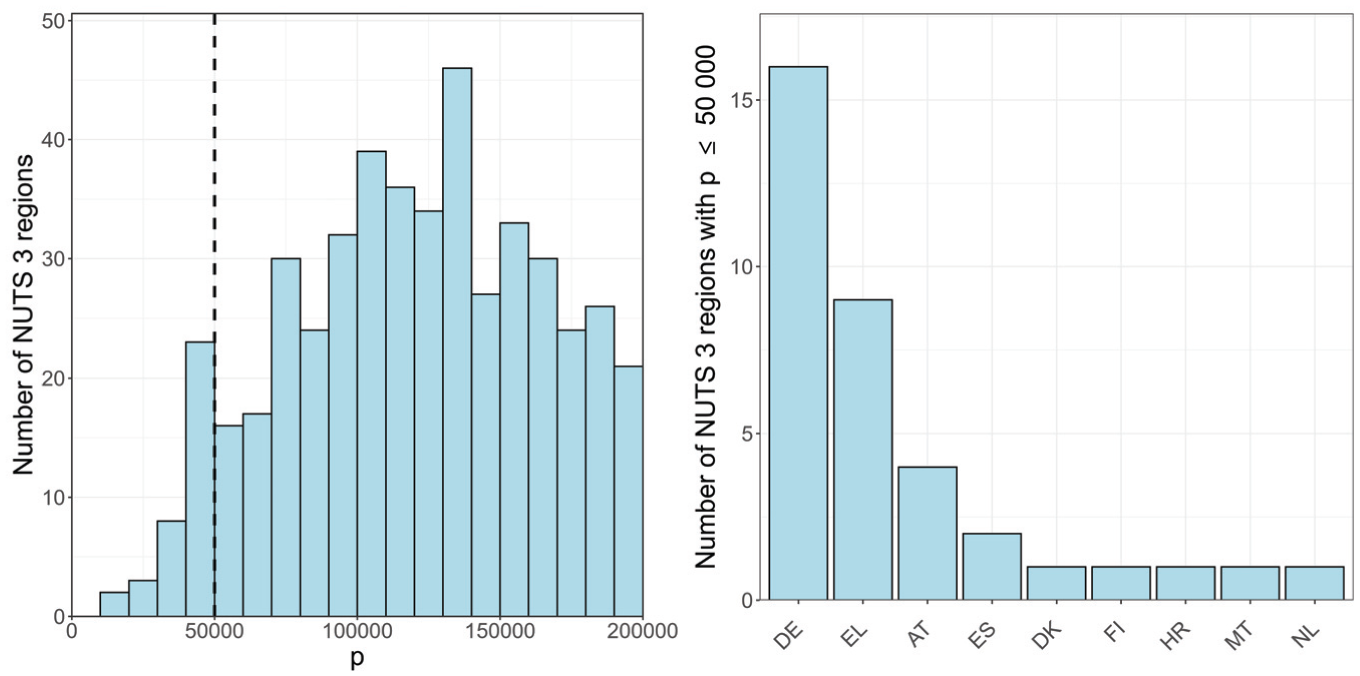
Even though the data sets analyzed here pertain to NUTS 2 level, these findings can be extrapolated to a NUTS 3 picture. This is due to the strong correlation of all uncertainties with population sizes that became explicit in the analysis above. The population sizes of the NUTS 2 regions in the ESS are distributed mainly between $200000$ and $3000000$ people with a center around $1000000$ people, whereas the NUTS 3 regions mainly lie between $10000$ and $500000$ people with a center around $120000$ people; see Figure 5. There are no NUTS 3 regions with a population $<10000$ people and in fact only five regions $<30000$ people. However, the regime of $30000$ – $200000$ people is covered by four NUTS 2 regions, and thus included in principle in the analysis above. This implies that the findings would hold in principle for NUTS 3 level indicators, too, including life expectancies—even though the age-specific indicators and underlying crude event counts considered here are currently not published at NUTS 3 level.

Figure 5.

Distribution of the total population $p$ of NUTS 3 regions on 1 Jan 2023 in the range up to $200000$ (left) and number of NUTS 3 regions with $p\le 50000$ by EU country (right).

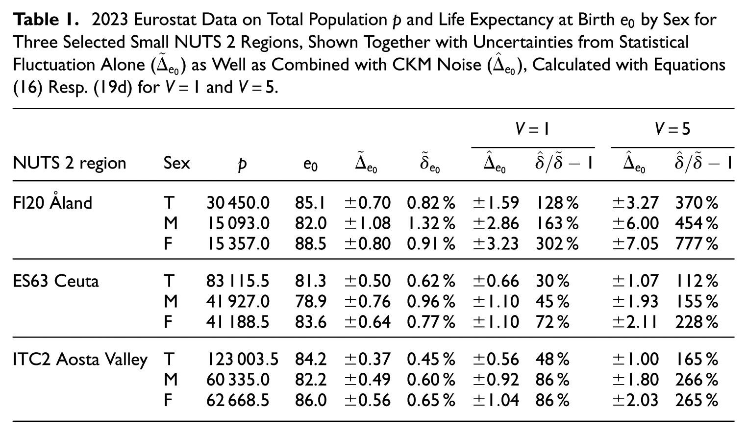
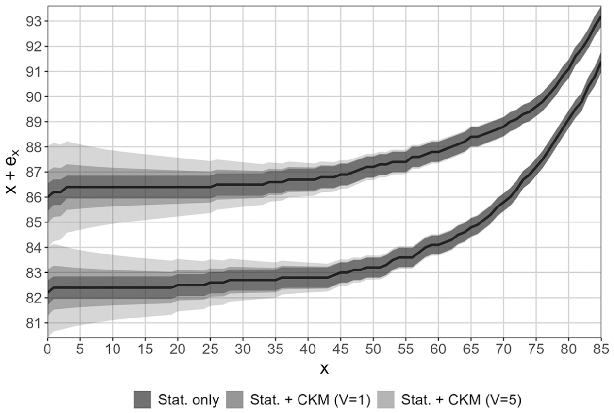
It therefore merits to have a closer look at those few NUTS 2 regions with total population $<200000$ people, as these may be seen as archetypal for NUTS 3 level results, where the previous analysis suggests to focus on life expectancy at birth $e_0$ . As detailed in Table 1, the noise contribution to the total uncertainty becomes relevant in this regime ( $\hat{\delta }/\tilde{\delta }-1>~50\mathrm{\%}$ ) even though statistical fluctuations remain very moderate ( $\tilde{\delta }<~1\mathrm{\%}$ ). This means that in this regime, $e_0$ is a statistically very accurate indicator which however receives notable additional uncertainty from noise protection of the underlying raw counts. This is also illustrated in Figure 6 showing the expected total years lived $x+e_x$ by sex including uncertainty bands for Aosta Valley ( $p\simeq 120000$ ). The graph is instructive as it visualizes some insights on uncertainties as a function of the age cohort: effects from protection noise with fixed variance are most relevant at $x=0$ , that is, for life expectancy at birth $e_0$ , and declining gradually to become negligible compared to statistical fluctuations above $x\simeq 45$ ; in contrast, statistical fluctuations remain a relevant uncertainty source for all ages.

Table 1.

2023 Eurostat Data on Total Population $p$ and Life Expectancy at Birth $e_0$ by Sex for Three Selected Small NUTS 2 Regions, Shown Together with Uncertainties from Statistical Fluctuation Alone ( ${\tilde{\mathrm{\Delta }}}_{e_0}$ ) as Well as Combined with CKM Noise ( ${\hat{\mathrm{\Delta }}}_{e_0}$ ), Calculated with Equations (16) Resp. (19d) for $V=1$ and $V=5$ .

						$V=1$		$V=5$
NUTS 2 region	Sex	$p$	$e_0$	${\tilde{\mathrm{\Delta }}}_{e_0}$	${\tilde{\delta }}_{e_0}$	${\hat{\mathrm{\Delta }}}_{e_0}$	$\hat{\delta }/\tilde{\delta }-1$	${\hat{\mathrm{\Delta }}}_{e_0}$	$\hat{\delta }/\tilde{\delta }-1$
FI20 Åland	T	$30450.0$	85.1	$\pm 0.70$	$0.82\mathrm{\%}$	$\pm 1.59$	$128\mathrm{\%}$	$\pm 3.27$	$370\mathrm{\%}$
	M	$15093.0$	82.0	$\pm 1.08$	$1.32\mathrm{\%}$	$\pm 2.86$	$163\mathrm{\%}$	$\pm 6.00$	$454\mathrm{\%}$
	F	$15357.0$	88.5	$\pm 0.80$	$0.91\mathrm{\%}$	$\pm 3.23$	$302\mathrm{\%}$	$\pm 7.05$	$777\mathrm{\%}$
ES63 Ceuta	T	$83115.5$	81.3	$\pm 0.50$	$0.62\mathrm{\%}$	$\pm 0.66$	$30\mathrm{\%}$	$\pm 1.07$	$112\mathrm{\%}$
	M	$41927.0$	78.9	$\pm 0.76$	$0.96\mathrm{\%}$	$\pm 1.10$	$45\mathrm{\%}$	$\pm 1.93$	$155\mathrm{\%}$
	F	$41188.5$	83.6	$\pm 0.64$	$0.77\mathrm{\%}$	$\pm 1.10$	$72\mathrm{\%}$	$\pm 2.11$	$228\mathrm{\%}$
ITC2 Aosta Valley	T	$123003.5$	84.2	$\pm 0.37$	$0.45\mathrm{\%}$	$\pm 0.56$	$48\mathrm{\%}$	$\pm 1.00$	$165\mathrm{\%}$
	M	$60335.0$	82.2	$\pm 0.49$	$0.60\mathrm{\%}$	$\pm 0.92$	$86\mathrm{\%}$	$\pm 1.80$	$266\mathrm{\%}$
	F	$62668.5$	86.0	$\pm 0.56$	$0.65\mathrm{\%}$	$\pm 1.04$	$86\mathrm{\%}$	$\pm 2.03$	$265\mathrm{\%}$

Figure 6.

Expected total years lived $x+e_x$ for NUTS 2 region ITC2 (Aosta Valley) shown as a function of age $x$ for each sex (upper line females, lower males). The uncertainty bands show intrinsic statistical fluctuations only (dark gray) as well as total uncertainty including a CKM noise contribution with variance $V=1$ (medium gray) and $V=5$ (light gray).

At this point it must be stressed that some notable impact of noise protection on the resulting accuracy should be acceptable in principle. After all, this merely exemplifies the fundamental trade-off between security and quality that is inherent to all disclosure control methods. From this perspective, relative noise contributions up to $\hat{\delta }/\tilde{\delta }-1~\mathcal{O}\left(100\mathrm{\%}\right)$ are not worrisome per se, especially if the noise protection allows in return to publish all raw counts and indicators without suppression.

Nevertheless, Table 1 shows the situation for a rather optimistic noise variance value $V=1$ . In practice, somewhat larger values in the range $V<~5$ should be more realistic. However, setting $V=5$ brings relative noise impacts to $\hat{\delta }/\tilde{\delta }-1>100\mathrm{\%}$ for all $e_0$ values in Table 1, and even to $400$ % to $700\mathrm{\%}$ (depending on sex) for the smallest region Åland (cf. lower-right plot in Figure 4), so here the SDC noise arguably starts to dominate the total uncertainty. Again, this should not be a reason to exclude noise protection but rather to apply particular care in analyzing the effects in-depth and selecting an appropriate $V$ value as soon as population sizes $\le 100000$ people come into focus.

In summary, the crude fertility and mortality rate indicators analyzed here do not add relevant accuracy constraints on the choice of the noise variance parameter $V$ for protecting the input population stock and event count statistics, as long as the range considered remains reasonable (e.g., $V\le 5$ ) and noise effects are considered together with intrinsic uncertainties from statistical fluctuations. On the other hand, findings on life expectancies suggest that noise protection effects should be examined closely for any population groups below $100000$ people, be it small NUTS 2 regions or other geographic units (e.g., NUTS 3, cities or functional urban areas), possibly split further by sex: Here the size of noise effects may exceed that of statistical fluctuations and statistical authorities may thus need to agree on certain accuracy thresholds that will then constrain their fine-tuning of $V$ . At this point it merits recalling that these findings are solely based on three basic properties of the protection noise, namely that it is sufficiently centered (bell-shaped underlying distribution), all noise terms are independent from each other and the noise variance is a fixed known value. The results are thus quite generic and hold for a whole class of noise protection methods with the mentioned properties, beyond the CKM used in this analysis.

6. Conclusions

This paper computes and analyzes the absolute and relative uncertainties on selected demographic indicators (age-specific fertility and mortality rates and life expectancies) when the raw input counts of births, deaths and population stocks are confidentiality protected by a generic noise method with fixed variance parameter $V$ . We obtain analytical expressions by applying uncertainty propagation based on linear response, as well as numerical results using demographic data published by Eurostat. To quantify the relative effect of noise protection, total uncertainties stemming from statistical fluctuations (according to a Poisson model) combined with additional noise uncertainties are compared to uncertainties only from statistical fluctuations.

The findings for combined relative uncertainties are that these become most pronounced in situations where the demographic indicator is dominated by very small raw input counts $<10$ . This is the case for crude age-specific fertility rates, where relative uncertainties can thus increase up to $100\mathrm{\%}$ for very small birth counts, and in particular for crude age-specific death rates, because small death counts are prevalent in many age bands. Vice versa, the relative uncertainties remain moderate ( $<10\mathrm{\%}$ ) and are often even negligible ( $<1\mathrm{\%}$ ) for more aggregated indicators like total fertility rates and age-specific life expectancies.

Regarding the relative impact of noise uncertainty, the analysis has shown that this remains negligible—that is, relative increase of total uncertainty compared to statistical fluctuation $<10\mathrm{\%}$ —for practically the entire relevant parameter space of all indicators analyzed. In general, noise effects become notable only in regimes where also the statistical fluctuations become large, even though the relative noise impact is bigger for life expectancies than for crude rates. While most results are calculated with $V=1$ , some additional variations with $V\le 5$ indicate that these conclusions generally hold for the whole $V$ range that is relevant in practice. However, for life expectancy at birth of small populations $\le 100000$ people with still small statistical fluctuations $~1\mathrm{\%}$ , the noise may start to dominate the combined uncertainty if rather large variances $V~5$ are chosen.

Finally, even though the relative uncertainties on all indicators correlate inversely with the population size, the present NUTS 2 level analysis includes in principle ranges $>~10000$ people so that the results are expected to also hold at NUTS 3 level or for other territorial typologies with a larger share of units with $10000$ to $200000$ people (e.g., cities or functional urban areas). It was shown that particular care needs to be taken here when fixing the noise parameter $V$ appropriately to limit the impact on the total uncertainty of life expectancy at birth.