
Abstract
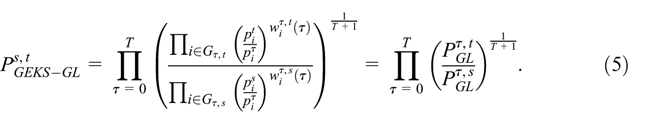
Price index decomposition allows the National Statistical Institute to break down aggregated price movements into contributions of individual commodities or product groups. In particular, decomposing multilateral indices, which combine many different time comparisons within the time window, can be useful in understanding and interpreting them by common users. This paper discusses multiplicative decompositions of multilateral GEKS-type indices, among which, currently, the GEKS-F and GEKS-T formulas are the most widely used. The paper also provides a multiplicative decomposition of the known GEKS-W index, as well as a decomposition of the GEKS-L, GEKS-GL, and GEKS-LM multilateral indices recently proposed in the literature. The paper also proposes normalized multiplicative decompositions of multilateral indices along with a relative commodity impact measure to enable comparisons of commodity contributions between products and across indices. The effects of these decompositions are demonstrated on two real scanner data sets from the food product segment.
1. Introduction
In modern inflation measurement, statistical agencies are increasingly turning to alternative sources of price data, including scanner and web-scraped data. Scanner data mean transaction data that specify turnover and numbers of items sold by bar-codes, for example, the Global Trade Article Number (GTIN), formerly known as the European Article Number (EAN), or Stock Keeping Unit (SKU) codes (Chessa 2015). As a rule, scanner data are obtained from electronic terminals of retail chains and their acquisition and processing is relatively cheaper compared to traditional price data collection. Scanner data have numerous advantages compared to traditional survey data collection due to the fact that such data sets are much bigger than traditional ones and they contain complete transaction information, that is, information about prices and quantities at the bar-code level. One of the main challenges when using scanner data is the proper choice of the price index formula which should take into account seasonal products together with new and disappearing goods (Eurostat 2018). Most statisticians agree that the optimal price index for measuring the dynamics of scanner prices is the multilateral index (Eurostat 2022). A multilateral index is compiled over a given time window composed of
Price index decomposition allows the National Statistical Institute to break down aggregated price movements into contributions of individual commodities or product groups. In particular, decomposing multilateral indices, which combine many different time comparisons within the time window, can be useful in understanding and interpreting them by common users. Nevertheless, the decomposition of multilateral indices is much more cumbersome and complicated than the decomposition of bilateral indices (Eurostat 2022). There are many papers in the literature discussing the decomposition of bilateral indices, for example, Vartia (1976), Reinsdorf et al. (2002), or Diewert (2002). For example, Balk (2004) discusses additive and multiplicative decompositions of the Fisher price index, and Hallerbach (2005) provides an alternative additive decomposition of this index that can be easily generalized to any bilateral price index formula that satisfies the linear homogeneity property. However, there is a lack of papers on decompositions of multilateral indices. For instance, Webster and Tarnow-Mordi (2019) provide decompositions for three multilateral methods: the Time Product Dummy (TPD) method advocated by Krsinich (2016), the GEKS method based on the Törnqvist (1936) price index (GEKS-T or CCDI)—see Gini (1931), Eltetö and Köves (1964), Szulc (1964), or Caves et al. (1982), and for the Geary-Khamis method proposed by Geary (1958) and Khamis (1972). Although Webster and Tarnow-Mordi (2019) give us a multiplicative decomposition of the GEKS-T (CCDI) multilateral index, they only state that the analogical decomposition for the GEKS-F index can be obtained “in a similar way, by substituting a multiplicative Fisher decomposition.” The multiplicative decomposition of the GEKS-F index, however, is not at all clear and obvious, as there are at least several multiplicative decompositions of the Fisher index. This paper suggests a particular form of this decomposition and discusses more widely the case with zero prices or unmatched products. Since GEKS-type indices occupy an important position and have earned a great deal of recognition among multilateral methods, and at the same time a multiplicative decomposition seems to be natural in their case due to the multiplicative form of the GEKS formula, this paper focuses on multiplicative decompositions of more or less well-known indices of this class. The paper compares the effects of these decompositions on real scanner data sets and in a simulation study. One of the novel results obtained in the study is the evaluation of the impact of the level of volatility in prices and volatility in consumption on the obtained decompositions of multilateral GEKS-type indices. It should be added that the paper considers the full thirteen-month time window, with no comparative analysis of product contributions when using index extension methods.
The structure of the paper is as follows: Section 2 lists more or less well-known GEKS-type indices, including recent proposals of the GEKS-L, GEKS-GL and GEKS-LM index methods, Section 3 provides multiplicative decompositions of all indices from the previous section along with their normalized versions, Section 5 is an empirical study that compares the above-mentioned GEKS-type index decompositions by using real scanner data sets, and Section 6 lists the most important conclusions of the research carried out.
2. The GEKS-Type Price Index Family
Let us denote sets of homogeneous products belonging to the same product group in the months
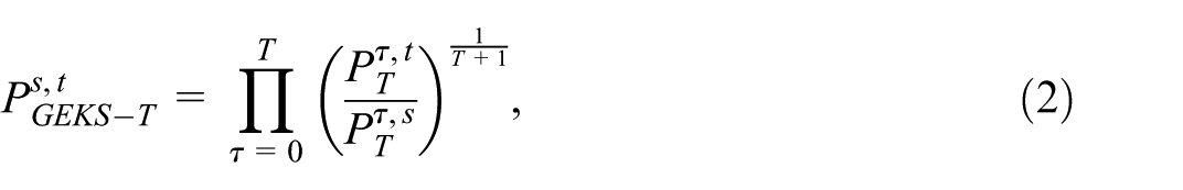
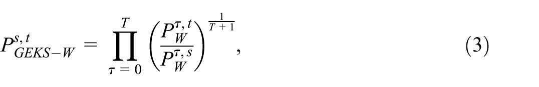
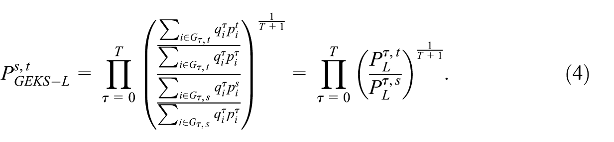
The GEKS price index between the months
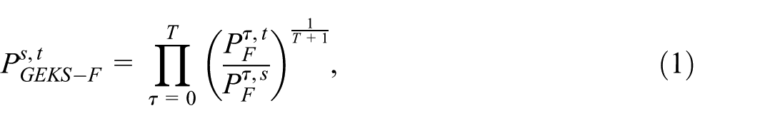
where
where
where
The latter one, the GEKS-GL index, is based on the geometric Laspeyres price index
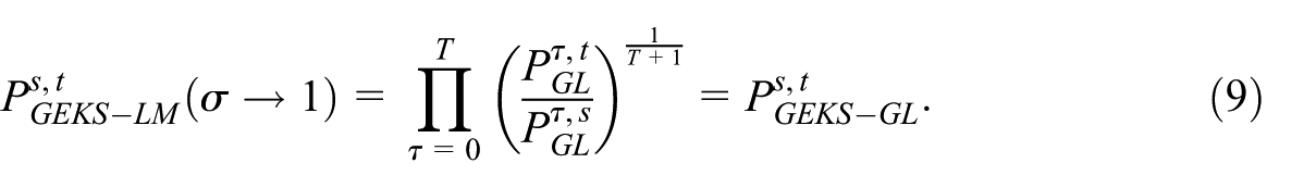
Also recently, a GEKS-type index based on the Lloyd-Moulton index has been proposed in the literature (Białek 2025). The Lloyd-Moulton price index (Lloyd 1975) can be written as follows:
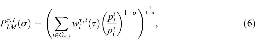
where the parameter
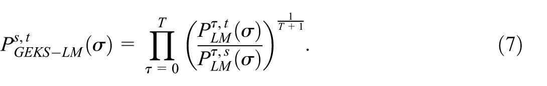
Please note that using the Lloyd-Moulton price index inside of the GEKS-type index is unconventional, since the Lloyd-Moulton index does not satisfy the time reversal test (von der Lippe 2007). Nevertheless, the GEKS-LM formula satisfies most tests for multilateral indices including the identity test (Białek 2025).
Since it holds that
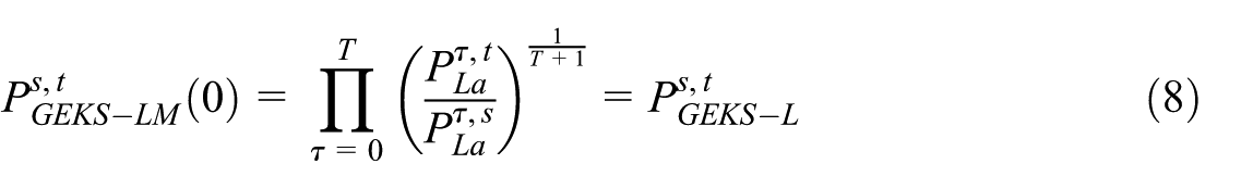
and
Nevertheless, the GEKS-LM index should be used after first determining the elasticity of substitution (
3. Multiplicative Decompositions of GEKS-Type Indices
This section provides multiplicative decompositions of more or less well-known GEKS-type indices. The choice of multiplicative decompositions as natural instead of additive is dictated by the fact that the GEKS index formula itself is also multiplicative.
3.1. Decomposing of the GEKS-T Index
As mentioned before, Webster and Tarnow-Mordi (2019) provide a decomposition of the GEKS-T index (known also as the CCDI index). On page 470 of the cited paper, a reader can find the decomposition formula for the case of missing prices and no missing prices. The authors equate the no missing prices variant with the case when “the same set of commodities is sold every period.” We believe that determining missing prices in this way is inaccurate and rather related to mismatched products. After all, scanned products can be perfectly matched over time and we can still observe missing prices (e.g., as a result of incomplete records in the database, resulting from erroneous data entry, incorrect data transfer, or other human factors). Even worse, there may be zero prices in the database, which will also distort the decomposition of the GEKS-T index (since zeros will appear in the denominator). Therefore, here we once again discuss the GEKS-T index decomposition supplementing it with special treatment of mismatched products.
In the presented paper, it will be assumed that after defining a homogeneous product (i.e., a level of data aggregation), records with zero prices (understood as unit value) and zero quantities are eliminated from the dataset. Please note that a promotion along the lines of “buy product X and product Y is bundled for free” means that zero prices and non-zero sales quantities may appear in the dataset. On the other hand, a product may have an unattractive price, and thus generate a lack of demand, in which case we observe a non-zero price but zero sales quantity. Both cases generate a technical problem in determining index contributions due to the impossibility of dividing by zero, and therefore the dataset should be reduced by such cases at the beginning of the procedure.
Under the significations introduced in Section 2, from Equation (2) we obtain that
where
Webster and Tarnow-Mordi (2019) suggest for the proposed decomposition of the GEKS-T index that “if there are any missing prices
and
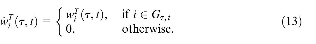
From Equations (12) and (13), we obtain that
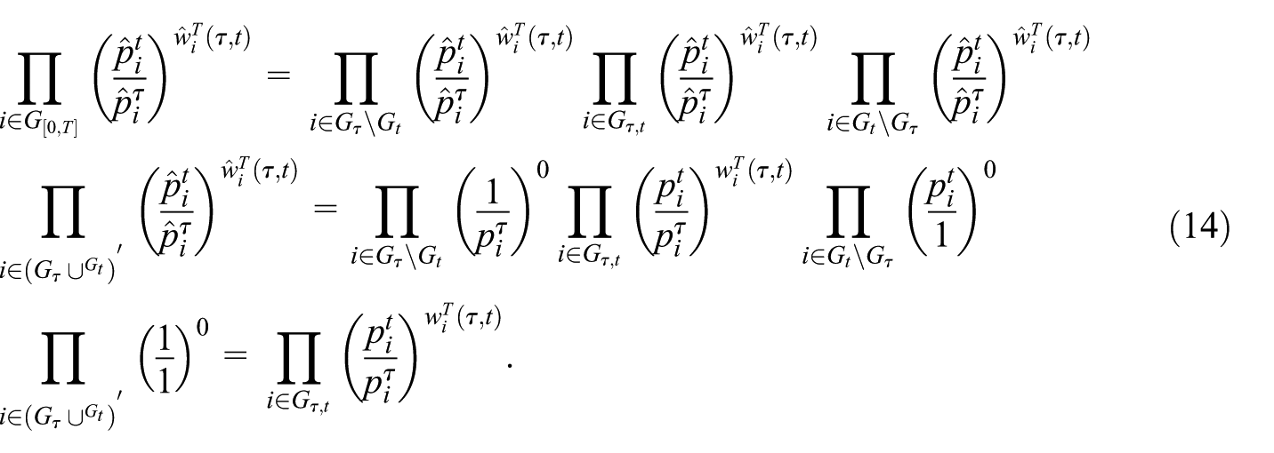
By analogy, it can be shown that
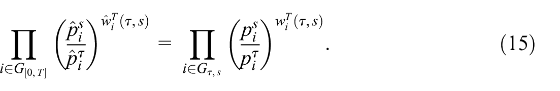
As a consequence of Equations (2), (14), and (15), we obtain that
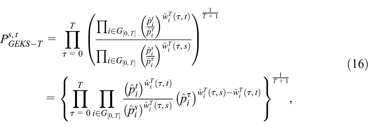
which, because of the iterator relative to
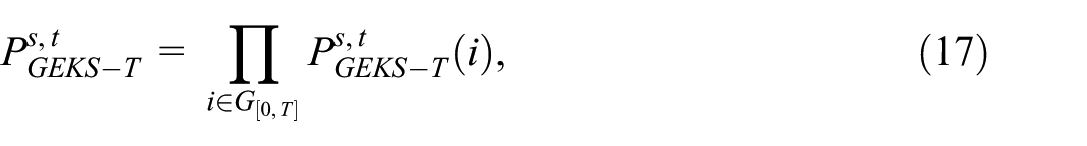
where

and
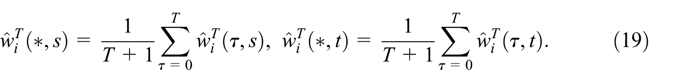
Please note that Equation (19) refers to Equation (28) in Webster and Tarnow-Mordi (2019) but we use here
3.2. Decomposing of the GEKS-F Index
In Webster and Tarnow-Mordi (2019), on page 470, we can read: “We could obtain a multiplicative decomposition of a GEKS price comparison in a similar way, by substituting a multiplicative Fisher decomposition into Equation 25.” The cited paper, however, does not propose a specific decomposition of the GEKS-F index, but only refers the reader to multiplicative Fisher index decompositions. The problem, however, is that at least several decompositions of the Fisher index can be found in the literature, but not all decomposition formulas contain weights that add up to unity. For instance, the sum of weights in one of the multiplicative Fisher index decompositions introduced in Vartia (1976) and demonstrated in Balk (2004; see Equation (12) on page 111) can be less than one. In what follows, the more satisfactory decomposition of the Fisher index that was obtained by Reinsdorf et al. (2002) and also recommended by Balk (2004) will be used. This multiplicative Fisher index decomposition is based on the Laspeyres (
where
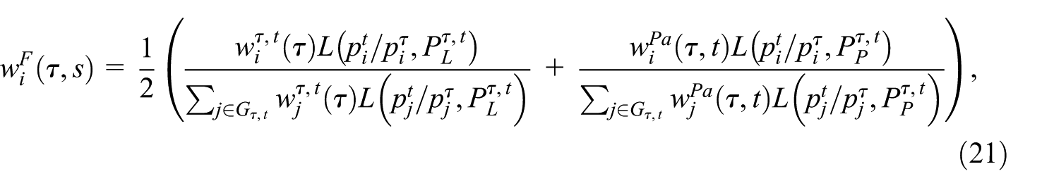
where
and
Let us use, similarly to Equation (13), the following signification:

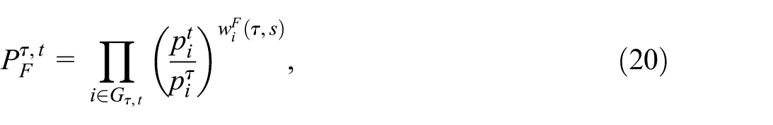
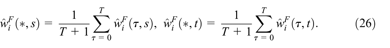
Using denotations Equations (12) and (23), we can obtain, analogous to Subsection 3.1, the following multiplicative decomposition of the GEKS-F index:
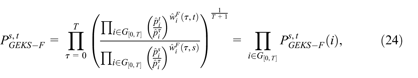
where
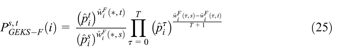
and
3.3. Decomposing of the GEKS-W Index
The Walsh (1901) price index, which compares the current period
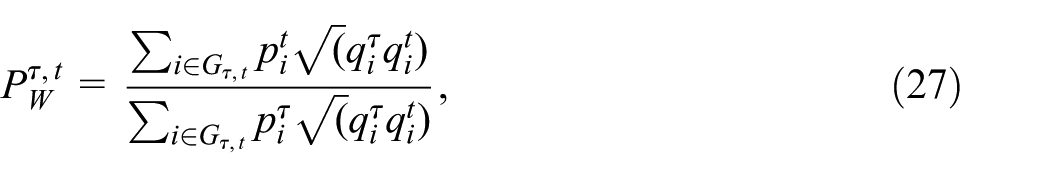
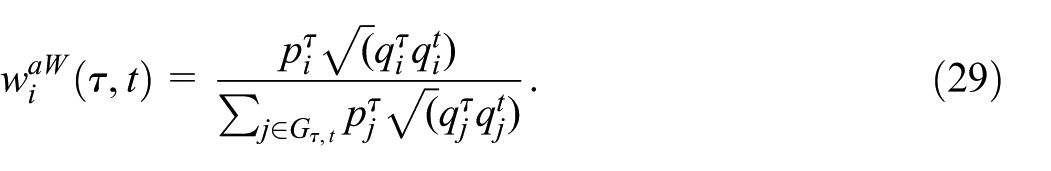
which allows us to write the Walsh price index as a weighted arithmetic mean of relative prices, that is:
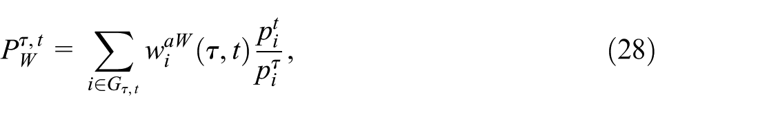
where
Balk (2008) showed that any weighted arithmetic mean of relative prices could also be written as a weighted geometric mean of relative prices. Following his method, we can express the Walsh price index Equation (28) as a weighted geometric mean of relative prices, that is:
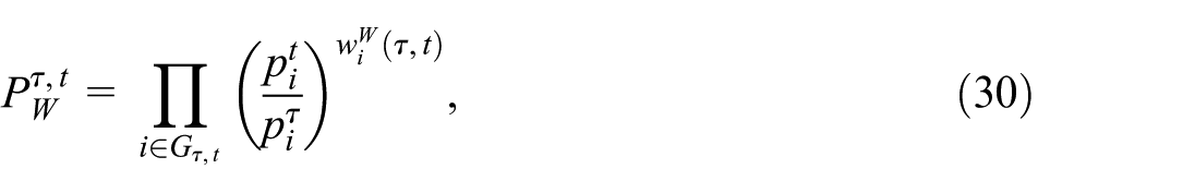
where
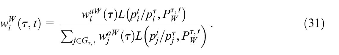
Let us use, similarly to Equations (13) and (23), the following signification:
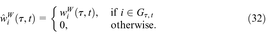
Using denotations Equations (12) and (32), we can obtain, analogous to Subsections 3.1 and 3.2, the following multiplicative decomposition of the GEKS-W index:
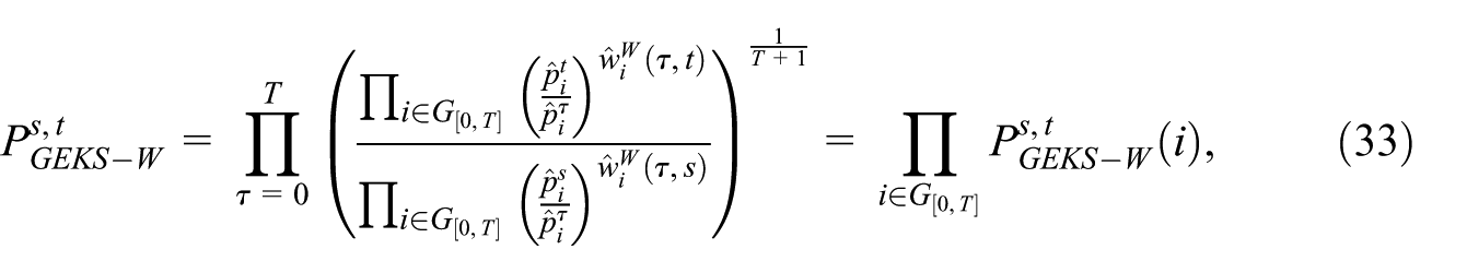
where
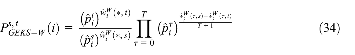
and
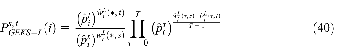
3.4. Decomposing of the GEKS-L Index
The Laspeyres (1871) price index
where
Let us use, similarly to Equations (13), (23), and (32), the following signification:
Using denotations Equations (12) and (38), we can obtain, analogous to Subsections 3.1, 3.2, and 3.3, the following multiplicative decomposition of the GEKS-L index:

where
and

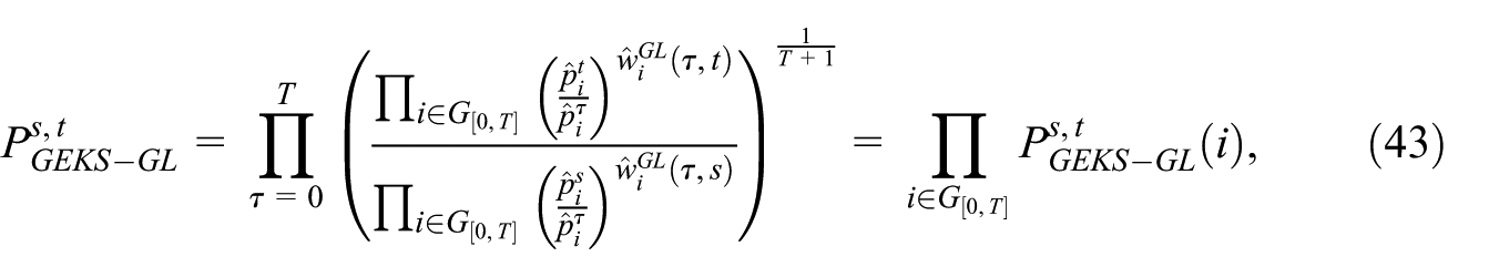
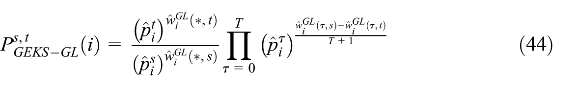
3.5. Decomposing of the GEKS-GL Index
The decomposition of the GEKS-GL index is somewhat simpler than the decomposition of other GEKS-type indices, since the geometric Laspeyres index is a weighted geometric mean of relative prices with fixed-base expenditure shares as weights (von der Lippe 2007). Let us use, similarly to previous sections, the following signification:
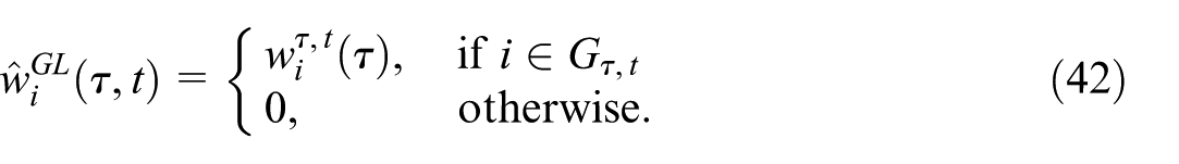
Using denotations Equations (12) and (42), we can obtain, analogous to Subsections 3.1, 3.2, 3.3, and 3.4, the following multiplicative decomposition of the GEKS-GL index:
where
and
3.6. Decomposing of the GEKS-LM Index
Firstly, please note that from Equation (6), we obtain
which means that, by using the above-mentioned Balk (2008) method, the formula on the left side of Equation (46) can be expressed as the following weighted geometric mean of amplified price relatives:
where
From (47), we have the immediate multiplicative decomposition of the Lloyd-Moulton price index:
Please note that
Let us use, similarly to previous sections, the following signification:
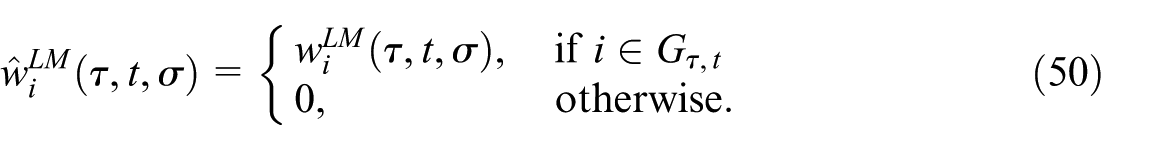
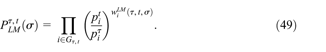
Using denotations Equations (12) and (50), we can obtain, analogous to Subsection 3.1 to 3.5, the following multiplicative decomposition of the GEKS-LM index:
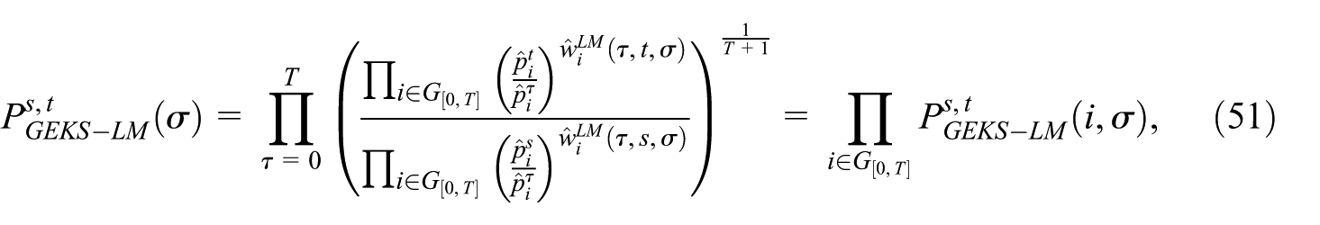
where
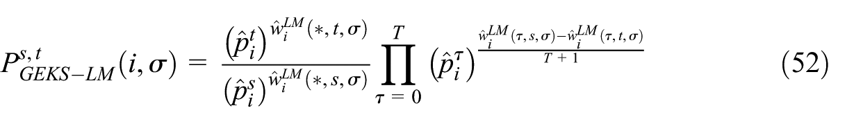
and
4. Comparing Decompositions Determined for Different Index Formulas
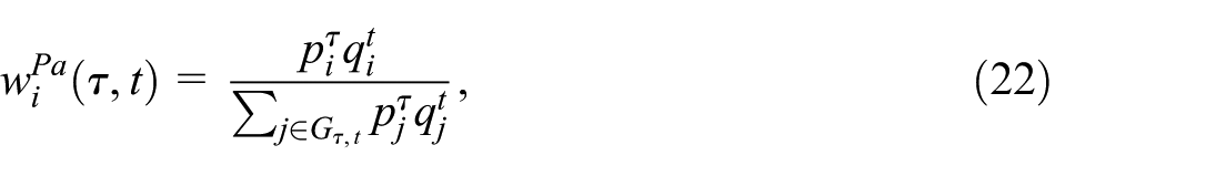
Comparing different decomposition methods within a single index is a seamless task. However, the task becomes more difficult if we want to compare the decompositions determined for different index formulas, since the contribution of a given commodity is not normalized by the index value. Therefore, in the paper, we propose the following simple solution to this problem. Assume that for the fixed base period and the current period, we want to compare the decompositions of the price indices
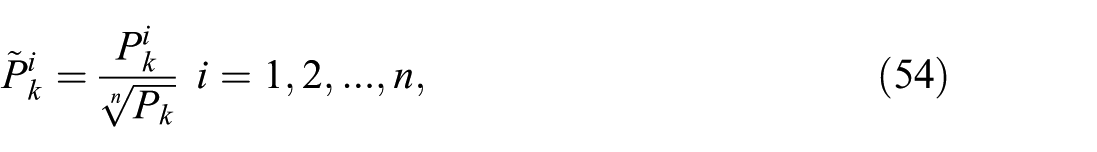
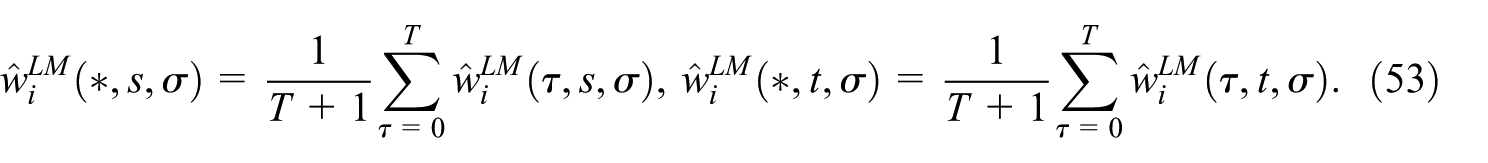
which are normalized to one, that is, we have
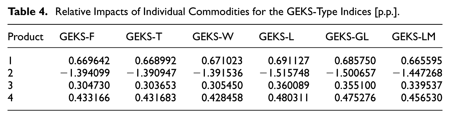
A comparison of the decompositions of the GEKS-type indices could also be made by determining the following relative impacts of individual commodities:

which determines the direction of the influence of commodities on the value of the price index. To better explain this, let us add that positive values of the relative impact of the commodity mean that the presence of this commodity in the CPI basket generates inflation, meanwhile negative values of the relative commodity impact lead to the conclusion that it generates deflation. The higher the absolute value of the relative impact of the commodity, the greater the impact of changes in the prices of this product on the values of the price index.
4.1. Example
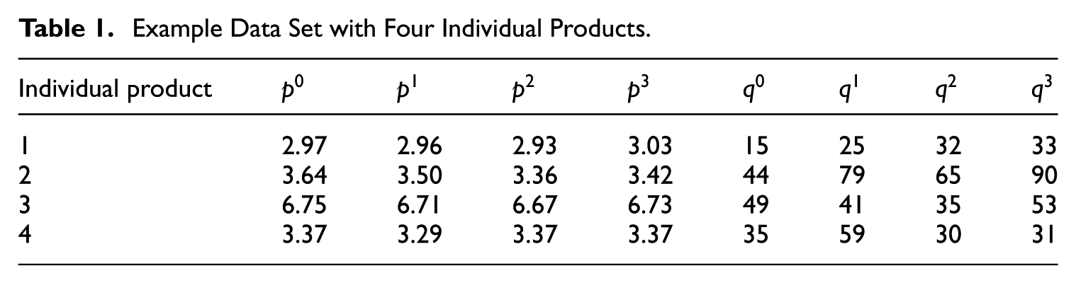
Let us consider a data set included in the publication by Eurostat (2022), that is, a data set concerning four individual products observed in four periods presented in the Table 1. By using algebraic methods (Białek et al. 2024), it can calculated that the elasticity of substitution for the base period
Example Data Set with Four Individual Products.
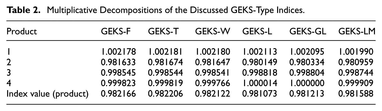
Multiplicative Decompositions of the Discussed GEKS-Type Indices.
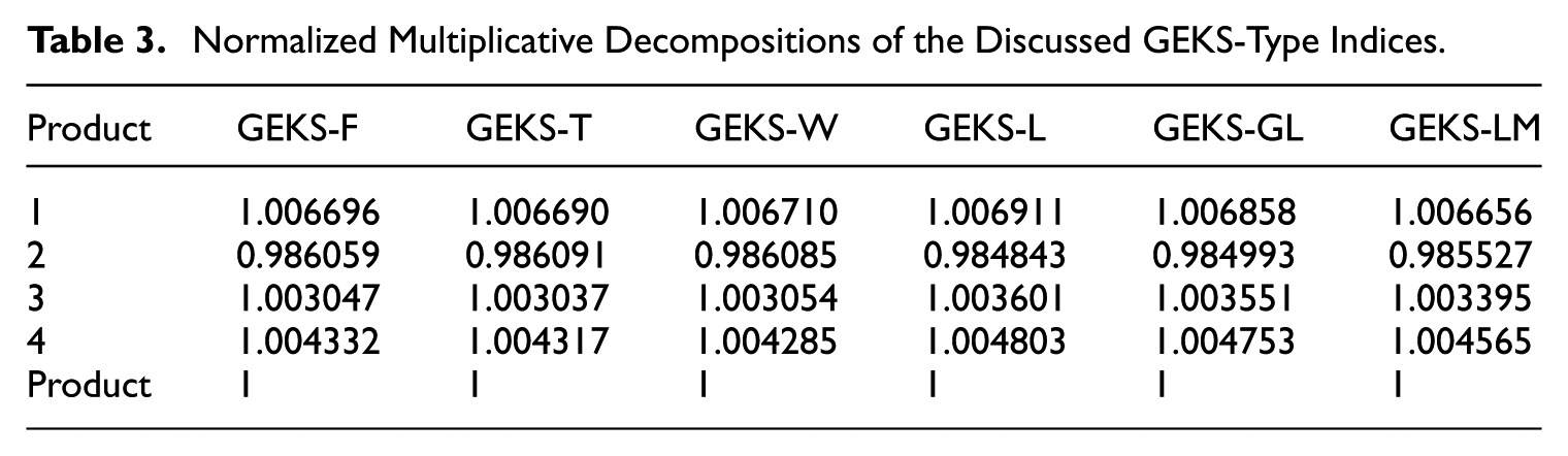
Normalized Multiplicative Decompositions of the Discussed GEKS-Type Indices.
Relative Impacts of Individual Commodities for the GEKS-Type Indices [p.p.].
5. Empirical Illustration
In the empirical study presented, multiplicative and (implicit) additive contributions for commodities, as well as relative impacts of products on considered GEKS-type indices, were determined. We use scanner data from one retail chain in Poland, that is, monthly data on coffee (COICOP 5: 01.2.1.1.1) and yoghurt (COICOP 5: 01.1.4.4.1) products sold in over 500 outlets during the period from December 2023 to December 2024. Two data aggregation levels have been used for index calculations, that is, the GTIN and COICOP 6 level. To be more precise: the COICOP 6-digit level means that the homogeneous product is defined one level lower than COICOP 5-digit level, that is, we then have broadly defined yoghurt products (e.g., drinking yoghurt, chocolate yoghurt, fruit yoghurt) and coffee products (e.g., ground coffee, instant coffee, coffee beans).
Before calculating the price indices, the data sets were carefully prepared. Product classification was performed using the
5.1. GTIN Data Aggregation Level
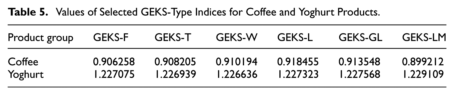
Table 5 presents values of full-window GEKS-type indices where December 2023 is the base period, December 2024 is the current period, and a thirteen-month time window is considered. Tables A1 and A4 provide multiplicative index contributions for twenty randomly selected coffee and yoghurt products. As mentioned before, such contributions are not relative to the value of the price index, and thus their comparative analysis between indices is hampered. Therefore, Tables A2 and A5 present normalized multiplicative index contributions for previously sampled coffee and yoghurt products. The elasticities of substitution needed to determine the GEKS-LM indices for the product subgroups under consideration can be found in Tables A7 and A8. Note that the elasticity of substitution values are noticeably different for different subgroups of products defined at the COICOP 6 level.
Values of Selected GEKS-Type Indices for Coffee and Yoghurt Products.
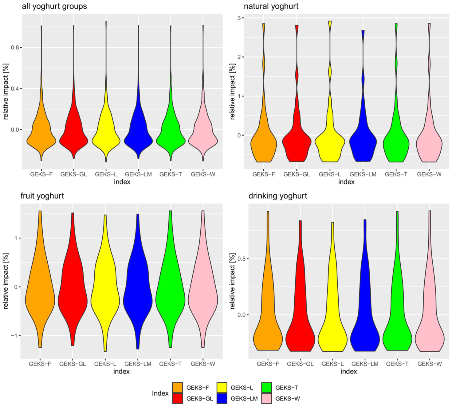
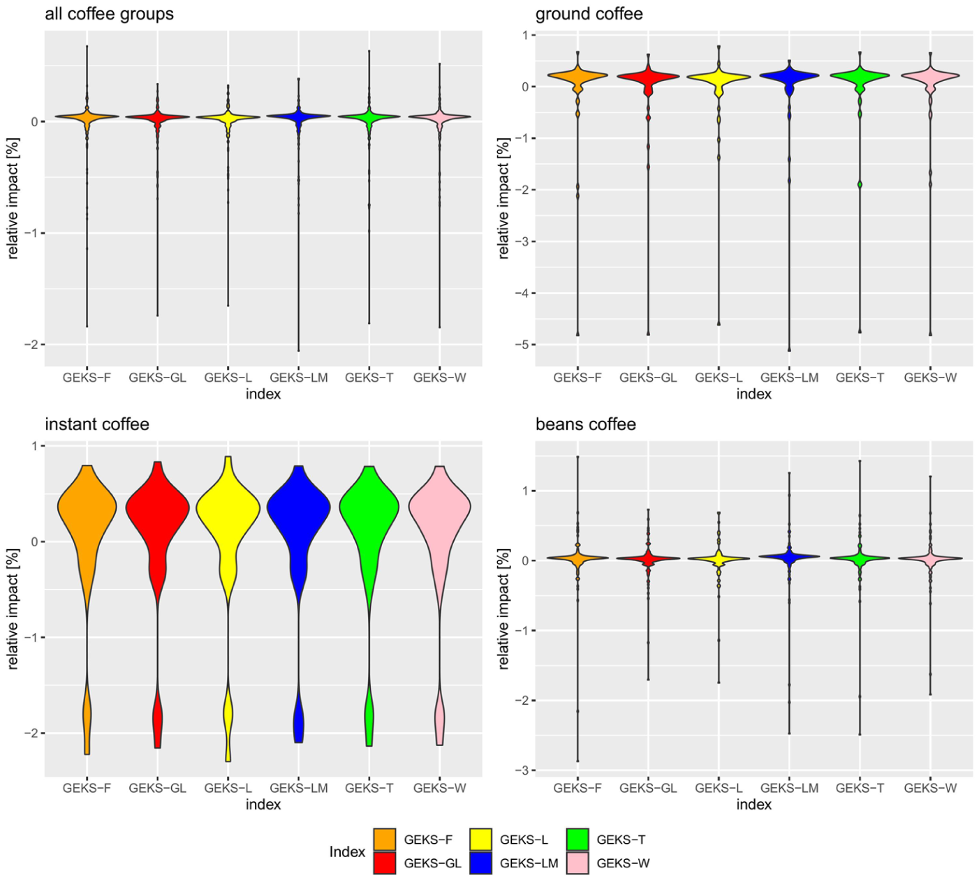
Additionally, Tables A3 and A6 present relative commodity impacts on the price index values for the same twenty randomly selected coffee and yoghurt products. The graphical comparisons of these relative impacts, that is, by using violin figures for all coffee and yoghurt products as well as for products from their COICOP 6 subgroups, are presented in Figures 1 and 2.
Comparison of relative commodity impacts for selected GEKS-type indices: coffee products.
Comparison of relative commodity impacts for selected GEKS-type indices: yoghurt products.
The detailed results presented in Tables A1 to A6 show that the contributions determined by the GEKS-F, GEKS-T, and GEKS-W formulas for most of the products are very similar. Also, the contributions for individual commodities determined by the GEKS-L and GEKS-GL formulas also approximate each other. This observation is apparent and reliable especially as we use the relative commodity impacts for this comparison, that is, the results from Tables A3 and A6. Additionally, we observe that the relative impacts values determined for the GEKS-LM index seem to form a separate, third cluster of values. In practice, however, differences between normalized index decompositions of the GEKS-type indices at the GTIN data aggregation level are of marginal importance (see Tables A2 and A5).
In the case of coffee products, despite the dominance of products with positive, albeit small, relative commodity impacts, due to the presence of a few percent of products with very large, negative relative impacts, the indices ultimately showed deflation in this product group (Table 5 and Figure 1). In the case of yoghurts, the situation is exactly the opposite. The dominant products here are those whose relative impacts on index value are small and negative, but a few percent of these products have very large, positive relative impacts (Table 5 and Figure 2). Consequently, the values of all GEKS-type indices determined for the yoghurt group are greater than unity indicating, averaging out, price increases.
5.2. COICOP 6 Data Aggregation Level
In this section, a homogeneous product is defined much more broadly than at the GTIN level, namely, the indentification of products here is done at the level of coffee and yoghurt grades (local COICOP 6 level). In the case of coffee, the following types were identified in the database: ground coffee, instant coffee, and coffee beans. For yoghurts, COICOP 6 levels were established for: natural yoghurt, fruit yoghurt, and drinking yoghurt.
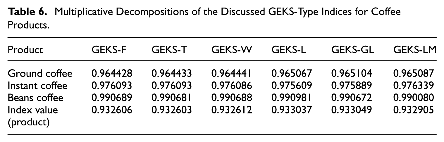
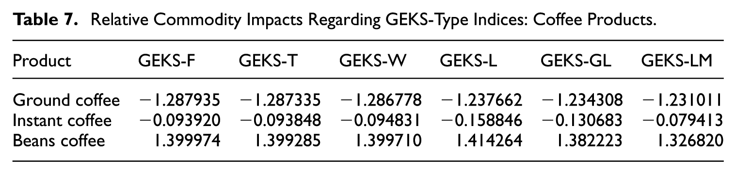
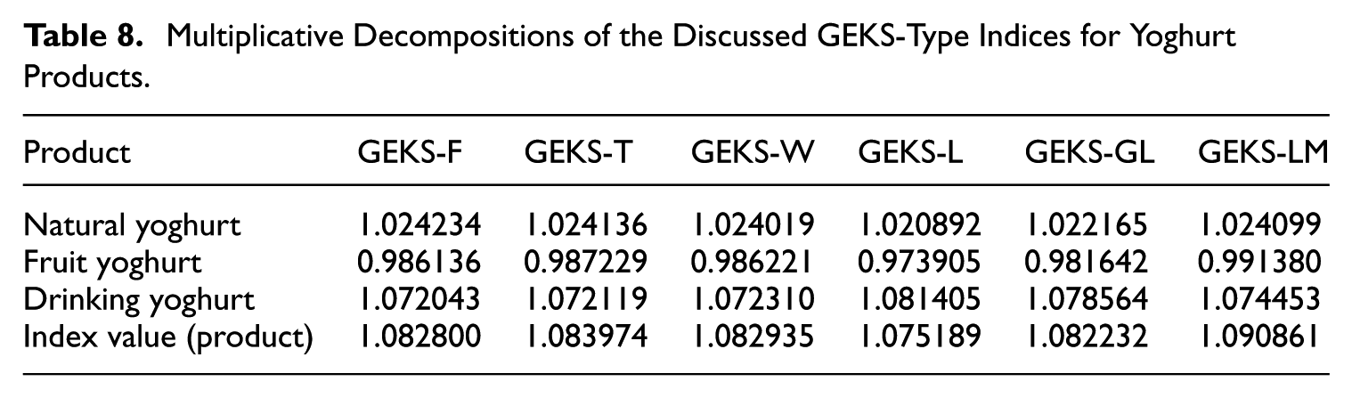
Tables 6 and 7 present multiplicative decompositions of the discussed GEKS-type indices and corresponding relative commodity impacts for coffee products. Similarly, Tables 8 and 9 present multiplicative decompositions of the GEKS-type indices and corresponding relative commodity impacts for yoghurt products. Normalized multiplicative GEKS-type indices decompositions for these product groups are presented in Tables B1 and B2.
Multiplicative Decompositions of the Discussed GEKS-Type Indices for Coffee Products.
Relative Commodity Impacts Regarding GEKS-Type Indices: Coffee Products.
Multiplicative Decompositions of the Discussed GEKS-Type Indices for Yoghurt Products.
Relative Commodity Impacts Regarding GEKS-Type Indices: Yoghurt Products.
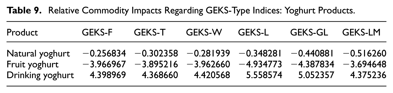
Results presented in Table 7 suggest that instant coffee and ground coffee products had a destimulating effect on the value of GEKS-type price indices, especially the ground coffee product generated large and negative relative impact values. The share of products for which the relative commodity impacts are negative here is so large (more than 63%) that ultimately their presence in the data set leads to deflation in the coffee group (all GEKS-type indices are below unity, e.g., the GEKS-F index equals 0.933). For the yoghurt group, relative commodity impacts are negative for natural and fruit yoghurt, while positive for drinking yoghurt. However, the share of the latter is so large in the sales of all yoghurts (more than 40%) that, in the end, the GEKS-type indices showed a surplus over 1 (e.g., the value of the GEKS-F index exceeded the 1.08 level).
It can also be noted that the differences between the normalized commodity contributions and the corresponding relative commodity impacts determined for the indices under consideration are clearly greater than the corresponding differences determined for the GTIN level (see results in Appendix B). However, as in Section 5.1, the comparison of relative impacts across indices leads to the conclusion that the decompositions of the GEKS-F, GEKS-T, and GEKS-W indices are very similar.
6. Conclusions
Decompositions of price indices into individual commodities are important from a practical point of view, as they allow the statistical office to assess the influence of individual products or groups of products in creating the value of the price index. In particular, the determination of commodity contributions allows the division of products into inflation- and deflation-generating groups. In the author’s opinion, multiplicative decompositions are more natural for GEKS-type indices than additive decompositions (which are also possible), since these indices are multiplicative.
This article provides multiplicative decompositions for more or less well-known GEKS-type indices, while systematizing and organizing the notation that can be found in the paper of Webster and Tarnow-Mordi (2019) in the framework of the GEKS-T decomposition. The added value of the paper is the multiplicative decompositions of the GEKS-L, GEKS-GL, and GEKS-LM indices, which have recently appeared in the literature and which are distinguished by the fact that they satisfy the identity test (Białek 2022b). Another added value of the article is the proposal of normalization of these multiplicative decompositions, as well as the proposal of relative commodity impact measures based on the normalized decompositions, which allow us to compare decompositions across different index formulas. All considered decompositions, their normalized versions, and relative commodity impacts were programmed in the R environment and included in the PriceIndices package. Note that the proposed decompositions, in particular the decomposition of the GEKS-L index, will be published in the latest edition of Guide on Multilateral Methods in the Harmonised Index of Consumer Prices (Eurostat 2022), which is currently in preparation. Further research on the discussed decompositions will also be presented at the next Ottawa Group Meeting to be held in Poland in May 2026.
The empirical study conducted provides two important observations, that is, that the multiplicative decompositions of GEKS-type indices depend substantially on both the data aggregation level and the level of elasticity of substitution. At the GTIN barcode level, the differences in individual product contributions determined for different index formulas may sometimes be substantially greater than the corresponding differences determined for the COICOP 6 level. At the same time, for a given GEKS-type index formula, the relative impacts calculated for products will be greater for the broader definition of a homogeneous product (COICOP 6).
The first effect can be explained if we notice that the mathematical formulas for product contributions determined for different GEKS-index formulas differ in the weight systems actually used within them. The weight systems are most often based on the logarithmic mean of relative prices and the appropriate bilateral price index formula. In other words, the more the bilateral price indices differ from each other, the more distances there are between the calculated contributions. As is known, bilateral price indices differ more as the level of price volatility increases. Therefore, in summary, the GTIN level, for which price volatility is much higher than for the COICOP 6 level, will generate greater differences in the determined contributions for individual commodities.
The second effect is apparent perhaps because the idea behind creating homogeneous subgroups of a COICOP 5 level group is that they contain the most “similar” products possible (to ensure the homogeneity of the subgroup) while highlighting the quality differences between these subgroups. Note that a similar idea is behind the classical clustering of objects by statistical methods. Since, as a result, we obtain subgroups of “similar” products in terms of quality, but, however, these subgroups differ from each other in terms of price and quantity levels, we can expect that the shares of these individual subgroups (more precisely: their relative impacts) in the formation of the price index will be noticeably different.
On the other hand, while assessing the impact of the elasticity of substitution, it can be seen that the thinner (with shorter whiskers) the violin charts for relative commodity impacts, the smaller the values of elasticity of substitution. Large values of substitution elasticity generated flattened violin charts but containing long whistles. It denoted abnormal (extremely large or small) values of relative impacts. Please note that in the paper, in accordance with the CES model, we assume that the elasticity of substitution is constant over the considered time window. However, the subject of the paper is not to discuss the validity of this assumption or the methods for estimating the elasticity of substitution. A more extensive discussion of the latter topic can be found in Białek et al. (2024).
An additional component of the conducted analyses involved a comparison of the computation times required to derive the considered price indices and their decompositions (see Appendix C). The comparison was carried out for both datasets presented in Section 5, with Tables C1 and C2 referring to the aggregation of data at the GTIN barcode level, while Tables C3 and C4 refer to the aggregation at the COICOP 6 level. Preliminary findings from this comparison suggest that, at the GTIN level, obtaining the decomposition is faster than estimating the corresponding price index in the case of the larger dataset (yoghurts), whereas it is slower for the smaller dataset (coffee). It should be noted that the yoghurt dataset consists of 501,439 records, whereas the coffee dataset contains 267,550 records. The most striking time savings, regardless of the data set, concern the GEKS-LM index. At the COICOP 6 level, the differences in computation times between the indices and their decompositions are minor. In fact, the times are in some cases more than twenty times lower than the corresponding times at the GTIN level. Interestingly, in this case the decomposition of the GEKS-LM index also results in a substantial reduction of the time required to determine the value of this index. To summarize this point, it appears that, under certain circumstances (e.g., when the dataset is very large), index decomposition may constitute a faster method for obtaining index values than their direct estimation.
It should be added that the paper considers the full thirteen-month time window, with no comparative analysis of contributions when using index extension methods. Although a thread related to the impact of the length of the time window was not addressed in the paper, one would expect it to be relevant. This is because, intuitively, as the length of the time window increases, the number of products included in the contribution estimation procedure also increases. Since at lower levels of data aggregation (particularly at the GTIN level) there is a high turnover of products and high variability in prices and quantities, a longer time window generally introduces even more of this variability into the analysis. Consequently, one would expect that as the length of the time window increases, the differences between the determined shares become larger. However, a thorough examination of this impact should be supported by a larger empirical study. This is a direction for possible further research by the author on the contributions of individual commodities.
However, the choice of methods for multilateral index extensions also seems to matter. Some of these methods shift the time window (e.g., splicing methods or Fixed Base Moving Window [FBMW] method), while others gradually expand the time window (Fixed Base Expanding Window Method [FBEW]). For a broader discussion of these methods, see, for example, the paper by A. G. Chessa (2019). Anyway, these two different approaches lead to two different sets of products considered in determining the expanded price index, so this must lead to differences in the levels of product contributions. Of course, the question arises about the magnitude of the differences obtained for the different choices of index extension method. This thread also requires further research, although some suggestions on the effect of splicing methods on differences in designated product contributions can be found in Webster and Tarnow-Mordi (2019; see Subsection 4.3 on page 479). For instance, these authors found that “the contributions of the commodities that are sold all year round follow the same ordering” (p. 483) and that some products, despite the fact that they were not sold in a certain period, still have nontrivial contributions to the rolling window index movements (e.g., peaches). However, it should be noted that in the paper cited above, the study focused only on fruits (i.e., apples, grapes, oranges, peaches, strawberries) and the only GEKS-type index included was the GEKS-T index. Thus, it seems that there is a need for further in-depth research on the impact of index extension methods on the formation of contributions of individual commodities.