
Abstract
Statistics Sweden employs a unique approach to higher-level aggregation of the Consumer Price Index (CPI). In the Swedish method, so-called “long-term links” are used to incorporate contemporaneous weight information into the index with a two-year lag. We compare this approach to the more standard method used for the European Harmonized Index of Consumer Prices (HICP), as well as to a long-term link variation of the HICP methodology. Our main focus is on year-on-year rates of change. This is motivated by the fact that, while long-term links by construction should improve the measurement of price change over longer time periods, effects on year-on-year inflation are less clear. In a simulation study performed on Swedish data, inflation rates are evaluated against a common benchmark measure. Several types of decompositions are also derived to help further explain differences and similarities between the methods.
1. Introduction
In a Consumer Price Index, household expenditure data is used to weight together price changes of various products into an overall measure. A practical problem that CPI compilers encounter is that expenditure information is typically available only with a certain time lag, while measures of inflation are required shortly after the end of the measurement period. Inflation estimates are therefore generally based on more or less outdated weights. Since people tend to adapt their consumption to price changes—buying more of goods and services exhibiting relatively smaller price increases, and less of those exhibiting larger increases—this risks leading to a positive bias in the CPI compared to an index based on a fully representative weighting structure (ILO et al. 2020, Chapter 8).
A possible solution to this problem is to revise the index as new expenditure information becomes available. In most countries, however, the CPI is not revisable (see e.g., ILO et al. 2020, 33). In Sweden, the government has specifically stated that it “takes for granted that the CPI will not be reconsidered after its completion” (Swedish Ministry of Finance 1993, author’s translation). Formally, this statement applies only to the CPI number itself and not to inflation estimates, but in practice, consistency in this respect has been prioritized by Statistics Sweden. The European harmonized inflation measure, on the other hand, is officially revisable (Eurostat 2024, 313) but revisions need to be specially agreed upon with Eurostat and are rare in practice.
In the absence of revision possibilities, one alternative is to complement the index with supplementary series providing more representative, although less timely, estimates of inflation to be used in parallel with the original CPI. A prominent example of this approach is the Bureau of Labor Statistics’ monthly weighted Chained CPI-U index (Cage et al. 2003; Klick 2018). Although in general, the publication of several parallel indices could create confusion among users, that should not be a big problem in this case as many countries already publish multiple measures of consumer side inflation today. Statistics Sweden, for example, produces the HICP, the CPI, and the CPIF (CPI with fixed interest rate). However, constructing additional measures will not prevent bias in the original series from accumulating over time. This could become an issue, especially if this index is used for compensation adjustments over a period of many years.
A third option for dealing with non-representative weights is through specific long-term links. This approach has a long history in Sweden and will be the focus of this paper. With long-term links, revisions are somewhat implicitly incorporated into later periods of a non-revisable series. Although the published figures are never changed, any bias in the index level is thus corrected for in the long run. A potential drawback of the approach, however, is that the long-term link adjustments will also affect month-on-month and year-on-year inflation rates. Clearly, optimality with respect to a long run level is not certain to translate into the best outcomes for rates of change. This aspect is particularly important for a statistic such as the Consumer Price Index, for which rates of change are key outputs for many users. (For example, in Sweden, year-on-year inflation according to the CPIF, which is compiled using the same higher-level aggregation methodology as the CPI, is used by the central bank to formulate its monetary policy target; see e.g., Sveriges Riksbank 2023.)
In Sweden, the idea of using long-term links was first proposed by a government commission of enquiry in 1953 (cf. SOU 1953; Statistics Sweden 2001; Ståhl 2024). At the time, the Levnadskostnadsindex (Cost of living index), a precursor to the Swedish CPI, was compiled as a chained Laspeyres-type index with yearly weights and linking over the December month. Each year, new weights were introduced with the December index. This practice was thought to minimize long-term bias since it allowed up-to-date weights to be used for the December links, but also made within-year comparisons more difficult. The 1953 commission argued that it would be preferable to have weight-shifts impacting only comparisons between different years. In particular, they gave the recommendation to introduce separate short- and long-term links for the December month; the short-term links would be constructed using the old weights and the long-term links using the new weights. The index for December could then be compiled using the short-term link while the long-term link would constitute the basis for the future index chain. In 1954, when the Swedish Consumer Price Index was created, this recommendation was put into practice.
The higher-level aggregation method of the Swedish CPI was reviewed again in the late 1990s, by another commission of enquiry (SOU 1999). This commission recommended to keep the long-term link principle—stressing that, even very small errors can, if they are systematic, accumulate to something significant over time—but to change the index formula to a “superlative” one, in the terminology of Diewert (1976); See Dalén (1999) for a detailed account of the commission's reasoning, and e.g., ILO et al. (2004, Chapter 17), for an introduction to superlative indices. In 2005, the long-term link formula of the Swedish CPI was therefore exchanged for a Walsh index.
In this paper, we compare the higher-level aggregation approach of the Swedish CPI to that of the Harmonised Index of Consumer Prices (HICP). The methodology of the harmonised index is similar to that used for the Swedish CPI before 2005, but without the long-term links. (Interestingly, the choice of higher-level aggregation method was not much discussed during its development; Astin 2021, 60, 132). The HICP is thus constructed as a chain of Laspeyres-type indices linked together over the December month, with weights set proportional to expenditure in a previous year. Since 2012, annual updating of the expenditure data is required (European Commission 2010; ECB 2012) but Statistics Sweden made yearly updates also before that. The Swedish HICP weights were first based on approximate expenditure data from the previous year, which was later changed into using more definitive data from two years ago.
In a comparison between the CPI and HICP aggregation approaches, simplicity speaks in favor of the HICP methodology. The current Swedish CPI approach, however, has the advantage of producing “unbiased” long run series as compared to a chain of superlative index links. This kind of unbiasedness has been viewed as particularly important in Sweden, because the Swedish CPI has a conditional Cost-Of-Living Index (COLI) as its theoretical target (Dalén 1999; SOU 1999). A Cost-Of-Living Index aims to measure the amount by which consumers would have to change their expenditures in order to “keep their utility level unchanged, allowing them to make substitutions between the varieties in response to changes in the relative prices” (ILO et al. 2020, 181). It can be contrasted to a Cost-Of-Goods Index (COGI), which instead aims to measure the changes in expenditure required to purchase the same, fixed, basket of products over time (e.g., ILO et al. 2020, 257). According to the so-called economic approach to index number theory, superlative indices can be expected to approximate COLI’s under fairly general conditions (cf. e.g., ILO et al. 2004, Chapter 17). Hence, superlative formulas are usually considered the optimal choice for COLI targets. Even for Cost-Of-Goods indices, however, superlative formulas are often viewed as the best option, although the interpretation of the corresponding bias becomes different (see e.g., Diewert 2002). For example, in a recent evaluation of the HICP (which is meant to be a COGI; European Commission 2016), the European Central Bank referred to a Törnqvist-like benchmark formula as an “optimally implemented COGI” (ECB, 2021). In this paper, we will simply view a superlative index as our operationalized target parameter. The potential advantages that come with using long-term links then becomes the same irrespectively of whether one intends to target a Cost-Of-Living or a Cost-Of-Goods Index.
Intuitively, the purpose of long-term links is to adjust, or rectify, the level of an index series compiled from only short-term links. We would thus expect the effect of long-term links to decrease with the relevance, or “up-to-datedness”, of the short-term weights. This issue is particularly relevant today because both the Swedish CPI and HICP have undergone methodological changes in this respect in recent years; during 2021 to 2024, the short-term weights of both measures were adjusted to better account for, in particular, Covid-19 related effects on household expenditures (Statistics Sweden 2025). In this paper, we will therefore consider two different methodological options for the short-term weights of the CPI and HICP aggregation approaches: Either basing them on two-year-old data or on more approximate information from the previous year. This corresponds to the methods used in practice by Statistics Sweden before and after 2021.
The rest of the paper is organized as follows. In Section 2, we introduce the different higher-level aggregation approaches. Month-on-month and year-on-year inflation rates are then considered in Section 3, where we also derive a decomposition of the corresponding formulas into so-called ``pure-price effects'' and ``reweighting effects''. Section 4 details the setup of the simulation study. In particular, a superlative-like year-on-year benchmark measure used to evaluate the aggregation methods empirically is defined, and the resulting error is decomposed into an ``estimation error'' and a ``formula error''. Simulation results are finally presented in Section 5, while Section 6 concludes.
2. Approaches to Higher-Level Aggregation
In the following, we will use the letter r to denote the first year of the index series and
The average price and total quantity associated with product, i.e., good or service, g in period t will be denoted as
2.1. The HICP Aggregation Approach
The Harmonized Index of Consumer Prices is constructed as a chain of short-term index links, each describing price change with respect to December of the previous year (Eurostat 2024, 272). In our notations, the structure can be written in the following way:
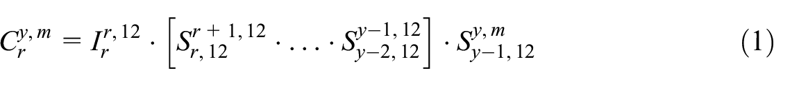
According to the legal framework of the HICP (in particular, articles 2.14 and 3.2 of regulation 2016/792 and article 3.1 of regulation 2020/1148; European Commission 2016, 2020), the short-term links should be compiled as Laspeyres-type indices. Moreover, the weights should be constructed mainly from National Accounts data from two years ago, but also “reviewed and updated to make them representative of [the previous year]”.
The following formula was used to compile the short-term links of the Swedish HICP between 2005 and 2020;
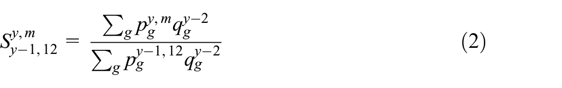
where the summations are taken over all products included in the index basket. (This simplified notation will be used throughout the paper.) Given the legal framework formulations, the implicit assumption behind the use of Equation (2) is that y–2 consumption can be considered ``representative'' also for year y–1. Shifting consumption patterns, however, made this assumption less likely to hold during the Covid-19 pandemic. (Eurostat 2024, 259; Lamboray et al. 2020.) Starting in 2021, Eurostat therefore recommended an alternative, adjusted, approach to the HICP weight compilations; Eurostat (2020, 2021, 2022, 2023). In line with these recommendations, Statistics Sweden shifted in 2021 into using indirectly calculated quantities referring to the previous year as basis for the HICP links. Hence, between 2021 and 2024, links were instead compiled in the following way:

In this paper, we will consider both of these alternatives and view them as corresponding to two separate aggregation methods.
2.2. The Current Swedish CPI Approach
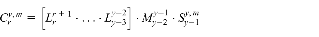
Turning to the aggregation structure of the Swedish CPI, it consists of a chain of long-term links, each describing price change between two consecutive years, and a final short-term link describing price change between the current month and two years ago. It can be written in the following way:
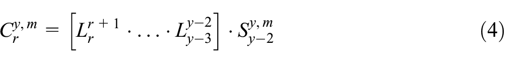
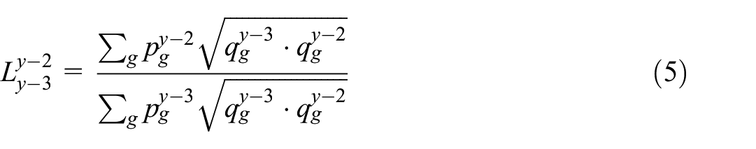
An important feature of the Swedish approach is that the index level will in the long run depend only on the long-term links. Since these long-term links are introduced with a two-year lag, contemporaneous expenditure data can be used to compile the corresponding weights. As already mentioned, the long-term links of the Swedish CPI are constructed using a Walsh index formula. The last link of the long-term chain in Equation (4) is thus given by:
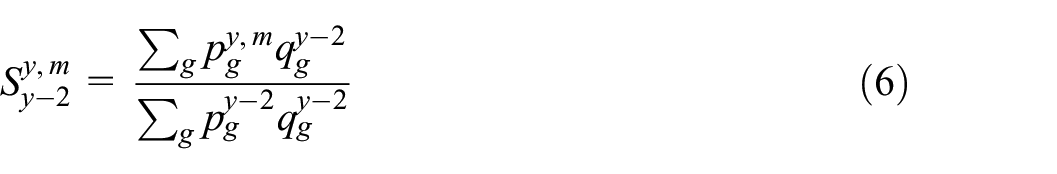
The short-term links of the Swedish CPI are in turn compiled as Lowe, or Laspeyres-type, indices. From 2005 to 2020, a true Laspeyres formula was used;
while an adjusted formula based on indirectly calculated quantities was employed between 2021 and 2024:
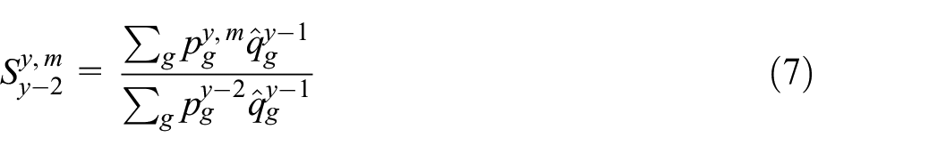
The primary reason for adjusting the short-term formula of the Swedish CPI in 2021 was to be consistent with the treatment used for the HICP. As a remark, however, we note that since the short-term links in this case extend all the way from year y−2 to the current month, the basket refers to the intermediate year of the price comparison. Equation (7) can thus be viewed as a kind of approximate “mid-year formula” (Diewert 2002; Hill 1998; Schultz 1998). In general, it would seem reasonable to assume for a mid-year formula to better approximate a symmetrically weighted (and hence, a superlative) index than Equation (6). Unfortunately, the volatility seen in connection with the Covid-19 pandemic made such assumption less likely to hold in 2021. (It can be noted that when first proposing the mid-year formula, Hill 1998 explicitly assumed “a fairly smooth transition […] in the quantities of goods and services consumed”.)
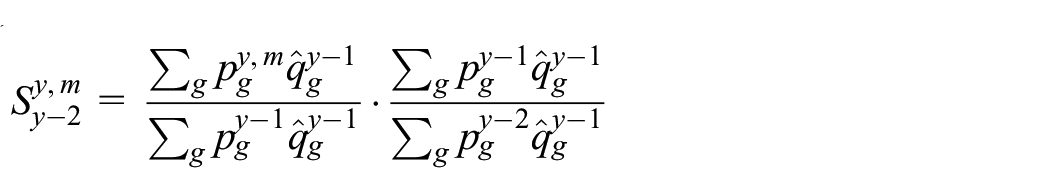
Other formulas were also considered for the Swedish CPI short-term links in 2021. We will include one of them in this paper. To describe this formula, note that Equation (7) also can be written as the product of a Laspeyres and a Paashe index (see also Okamoto 2001):
Hence, an obvious alternative would be the product of a Laspeyres and a Walsh index:
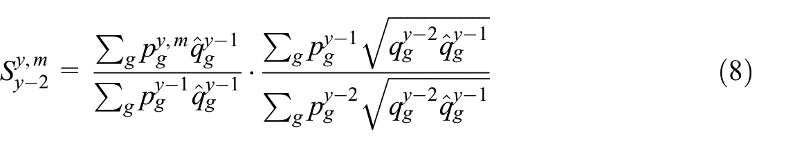
This alternative fits better into the overall structure of the Swedish CPI, as given by Equations (4) and (5), and was also the first option discussed at Statistics Sweden at the time. (Its main drawback, however, was that it could not be easily implemented into the production system on a short notice.) We will include this alternative as part of our study.
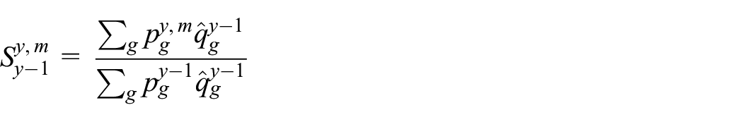
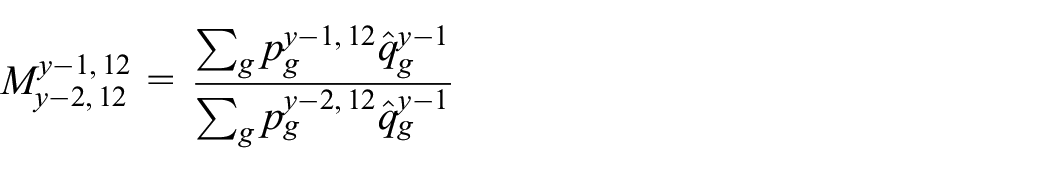
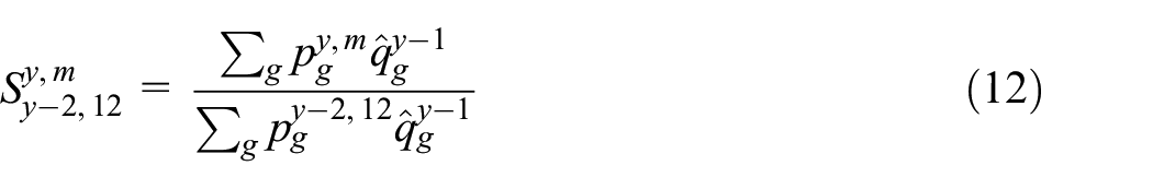
As a final remark, we note that Equation (8) also can be described in a different way. Since the second factor of Equation (8) is compiled using the same index formula as the long-term link but with more approximate quantities, it can be viewed as a kind of ``preliminary long-term link'', or ``medium-term link''. In the following, we will denote such a link by the letter M. We can thus rewrite the chaining structure corresponding to Equation (8) as
with
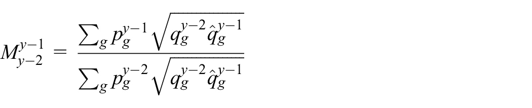
and
We will come back to this idea of medium-term links later in the paper.
2.3. The Previous Swedish CPI Approach
Finally, we turn to the aggregation approach used in Sweden between 1954 and 2004. Since this method combines the use of long-term links with December chaining, it can be described as a mixture between the previous two approaches. In the following, we will therefore also refer to it as the “mixed approach”.
In general, a chaining structure with December long-term links can be written:
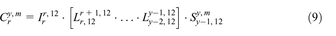
In this case, the long-term links describe price change from one December to the next and are compiled with a one-year lag. In the Swedish CPI, approximate expenditure data from the previous year was used to compile these links. This implies the following formula for the last link of the long-term chain in Equation (9):
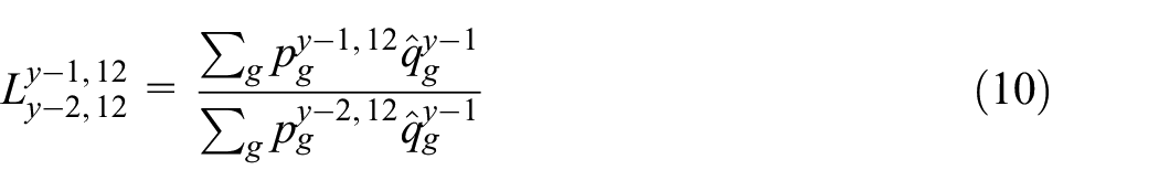
Similar to Equation (7), Equation (10) can be described as a kind of approximate mid-year formula. (This particular formula is also discussed by von Hofsten 1952, 11–12.) The short-term links of the mixed approach can in turn be compiled using any of the formulas used within the HICP approach. In this paper, we will focus on Equation (3) for this aim, since this corresponds most closely to how these links were compiled in practice by Statistics Sweden at the time.
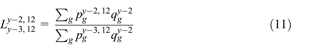
Finally, we will also include an alternative version of the mixed approach in our evaluations. To see the point of this alternative, note that a potential drawback of using Equation (10) to compile long-term links is that this index formula is based on indirectly calculated quantities. This means that indirect quantity estimates will remain in the chained index permanently. To circumvent this problem, a kind of medium-term link can be introduced. We can thus use the following alternative structure;
with
and
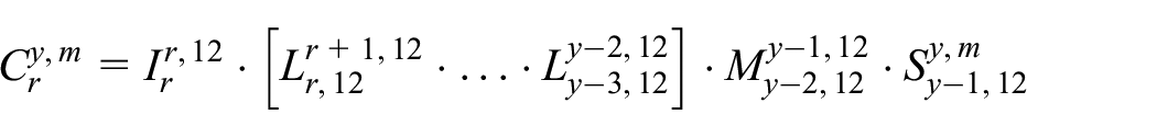
Below, we will write this alternative version of the mixed approach as a function of a two-year short-term link, to be consistent with the presentation of the other methods. In other words, we will have;
and
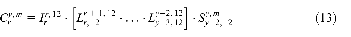
for the alternative version.
2.4. Overview of Higher-Level Aggregation Methods
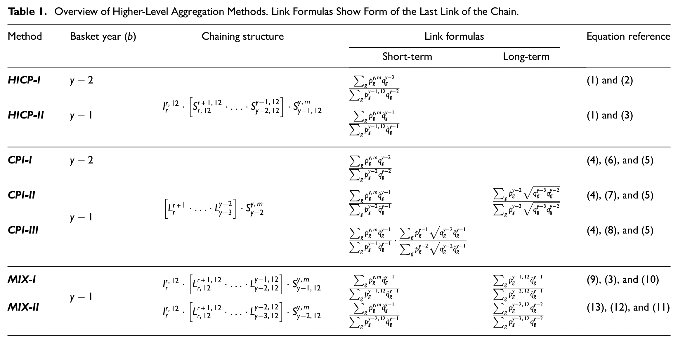
Table 1 summarizes the higher-level aggregation methods to be evaluated in the paper. In the following, we will refer to them by the names given in the first column of this table. The second column specifies the reference year of the quantities used for the short-term links. We will refer to this as the “basket year” of the method and denote it by the letter b. In the next section, we look further into the corresponding formulas for rates of change.
Overview of Higher-Level Aggregation Methods. Link Formulas Show Form of the Last Link of the Chain.
3. Formulas for Rates of Change
We now turn to year-on-year and month-on-month inflation and examine the form that these rates of change take when using one of the aggregation methods listed in Table 1 to compile the chained index. In the following, we will use
and

Moreover,
and
Obviously,
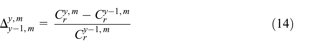
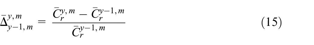
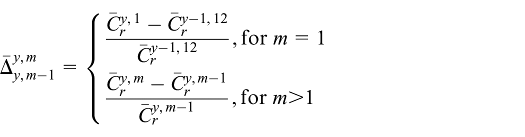
In the simulation study presented later, we will compare year-on-year inflation rates compiled according to both Equations (14) and (15) to a superlative-like year-on-year benchmark. In this section, however, we focus on
3.1. Pure-Price and Reweighting Effects
We start by decomposing the formula-related rates of change,
The pure-price effects corresponding to the year-on-year and month-on-month rates of change will be denoted as
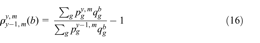
and
For example, if method HICP-I is used to compile the index, the pure-price effects will be defined with respect to a basket of year y−2 quantities, whereas a basket of y−1 quantities will be used if method HICP-II is applied.
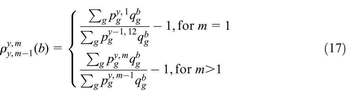
In order to define the corresponding reweighting effects, we need one additional notation. In the following, we let
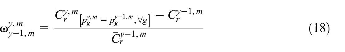
and
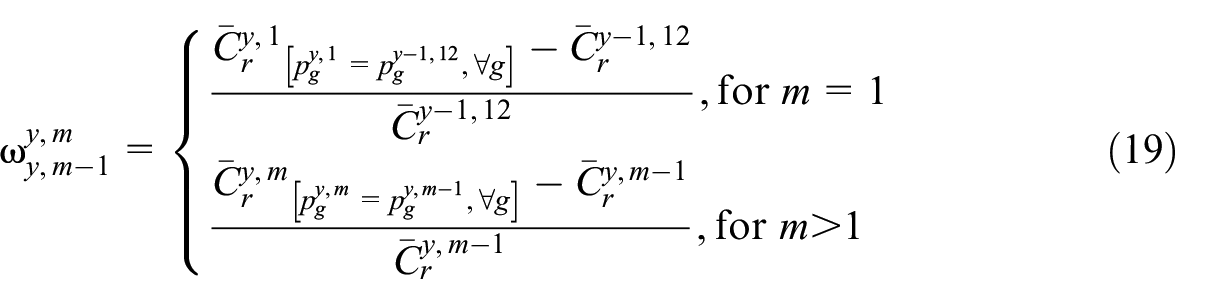
Intuitively, the reweighting effects can be thought of as hypothetical inflation rates; for example, Equation (18) gives the year-on-year inflation that would be obtained from the compilation process if all prices happened to be the same as one year ago (and indirectly calculated quantities were equal to the direct ones). A similar interpretation can be given to Equation (19).
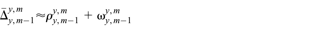
Combining Equations (16) and (17) with Equations (18) and (19), we obtain the following decompositions of
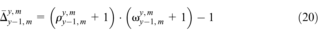
and
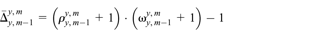
Corresponding easier-to-work-with approximate formulas are given by:
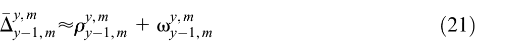
and
Using these formulas, the rates of change are thus decomposed into a pure-price effect—which depends only on which basket is being used for the short-term links—and a reweighting effect—which captures the impact of changing short-term weights between years and of introducing any new long-term links into the chain.
Of course, pure-price and reweighting effects could also have been defined in other ways. For example, Knetsch et al. (2025) make the point that a weight-based approach, that is, an approach where the equivalent of the pure-price effect keeps weights rather than quantities fixed, has advantages when making comparisons between countries or time periods with differing weight compilation strategies. At Statistics Sweden, formulas like Equations (18) and (19) are currently used to communicate effects of yearly updates in the CPI to the public. (In this communication, the formulas are, however, applied to
3.2. Reweighting Sub-Components
Next, we will look more closely at the reweighting effects associated with the seven aggregation methods listed in Table 1. To highlight differences and similarities between the methods, we will further decompose these effects into several sub-components.
Table 2 lists the sub-component decompositions that will be used below. The first column shows the decomposition of the year-on-year reweighting effect, and the second column that of the month-on-month reweighting effect in January. (For February to December, month-on-month reweighting effects are zero for all methods considered in this paper.) Because the sub-components can be classified as being of three different “types”, we have used the letters A, B, and C to denote them in the table. (Note also that since the two versions of the mixed approach differ from each other only in their use of indirectly calculated quantities, their reweighting effects—and hence, the corresponding sub-components—are identical.)
Decomposition of Reweighting Effects into Sub-Components.
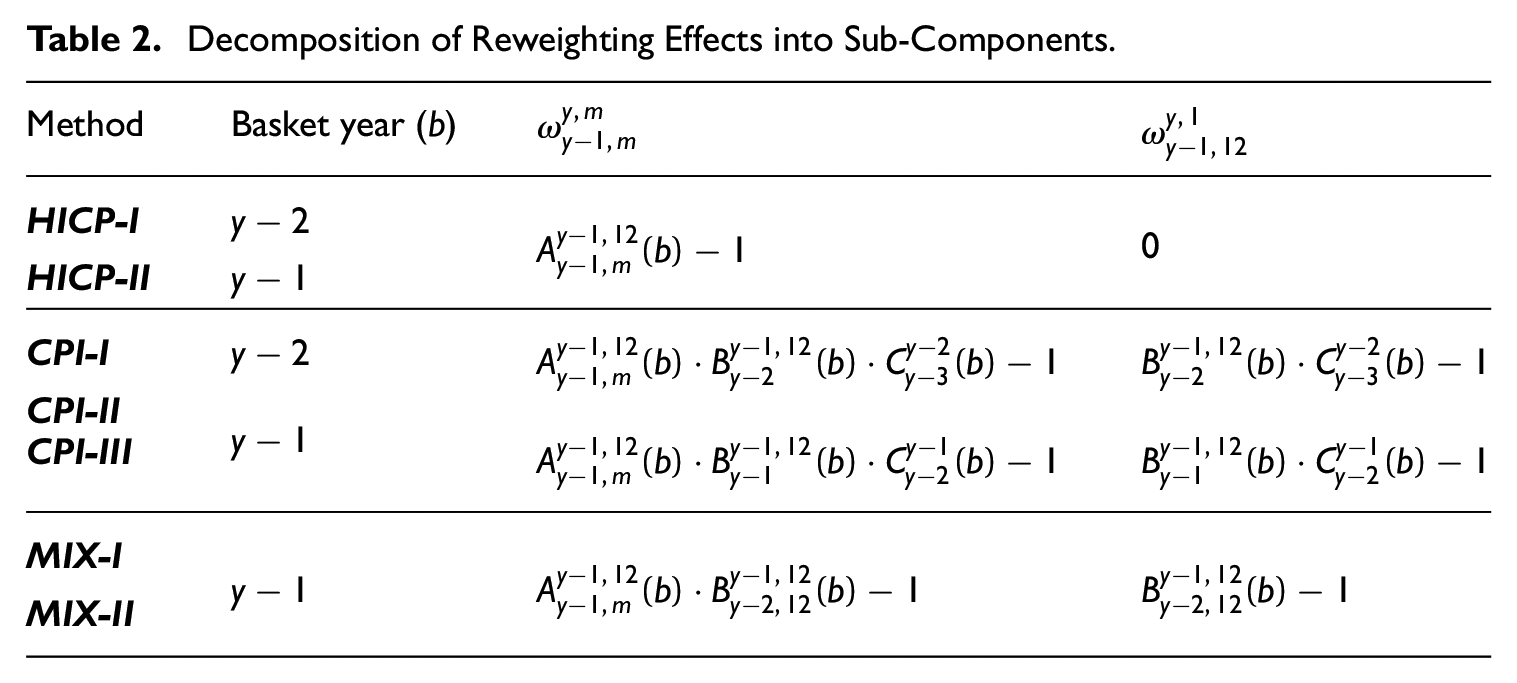
Definitions of the A, B, and C-type sub-components will be given below. First, however, we make a few preliminary observations from the overall presentation in Table 2. One thing that can be noted is that the same kind of A component,
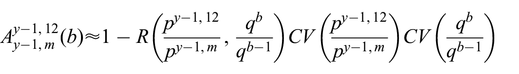
Next, we will specify the form of the reweighting sub-components in explicit terms. Starting with the A-type component, we will define this as the ratio of two different Lowe indices. While both indices describe price change for the same period, that is, between months m and 12 of year y−1, they will be based on different baskets. The numerator index will weight prices with year b−1 quantities, and the denominator index with quantities from year b. In other words, we have the following definition:
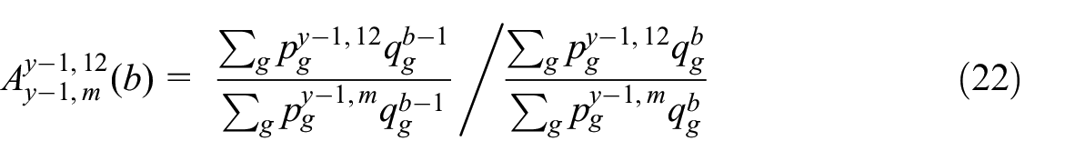
This sub-component is most easily interpreted in the context of the HICP approach, where it constitutes the full reweighting effect. Since we have defined the pure-price effect in terms of the “current” basket, that is, the one from year b, the A component captures the fact that in the chained index of Equation (1), price changes from period y−1,m to y−1,12 are actually incorporated based on the basket of year b−1.
In most cases, we would expect for the numerator of Eqution (22) to be on average larger than the denominator, and hence, for
where
In practice, since
The second type of sub-component, denoted by the letter B in Table 2, will also be defined as the ratio of two Lowe indices. In this case, however, the denominator basket will be the older one. The numerator index will thus be based on basket year b and the denominator index on b−1. For example, the B component included in the reweighting effects of methods CPI-I and CPI-II, which depends on price changes between year y−2 and December of year y−1, will be defined in the following way:
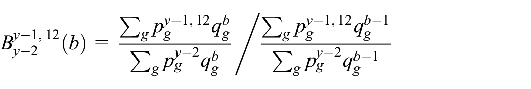
(The other B-type sub-components will have the same form, but with y−2 prices replaced by either y−1, for CPI-III, or y−2,12, for MIX-I and MIX-II.) An alternative expression is given by:
In this case, a negative correlation between price and quantity changes would lead to the sub-component being smaller than one. Since a similar expression can be obtained for all B-type sub-components, these components will all tend to have counteracting effects compared to the A components.
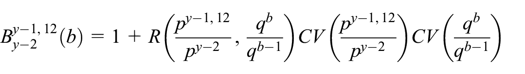
The B sub-component which is most interesting to analyze in its own right, is the one present for the mixed approach:
This sub-component describes the impact of the long-term links on the rates of change of the mixed approach. More specifically,
The joint effect of the A and B sub-components is for the mixed approach equal to:
For this aggregation approach, the total year-on-year reweighting effect would thus usually be expected to be negative, especially toward the end of the year when the A sub-component approaches one.
For the CPI approach, the A and B sub-components are preferably analyzed together. For CPI-I and CPI-II we can write;
which means that the joint effect will be a B-type effect for price changes between year y−2 and month m of year y−1. This joint effect will capture the effect of price changes between y−2 and y−1,m being incorporated into the chained index of Equation (4) based on the year b basket, instead of based on the basket from year b−1 (which was the case during the previous year). We would usually expect for it to affect rates of change downwards.
For CPI-III, we obtain instead:
This is again a B-type effect, but this time with a more unclear sign. We would mainly expect for it to reflect the within-year pattern of
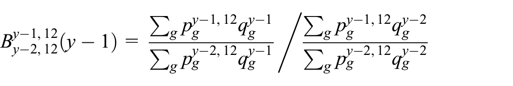
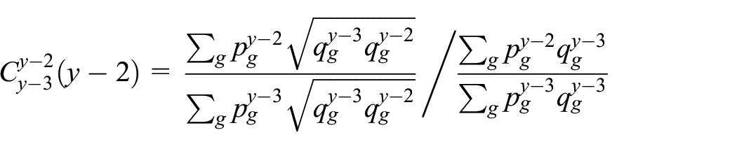
For the CPI approach, a bias correction interpretation similar to the one made for the B-component of the mixed approach is most easily given to the C-type sub-components. These components will be defined as ratios of Walsh and Lowe indices, with the Lowe index being based on b−1 quantities. In particular, the sub-components included in the reweighting effects of methods CPI-I and CPI-II will be defined as;
and the component present for method CPI-III by:
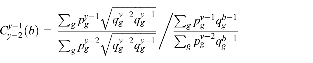
The C components of methods CPI-I (with b=y–2) and CPI-III (with b=y–1) thus have the same form, only that the latter is “postponed” one year. For method CPI-I,
This component can be thought of as retroactively (i.e., in year y) correcting for a bias which otherwise would have occurred in the measurement of price changes between year y−3 and y−2. The corresponding alternative expression is given by
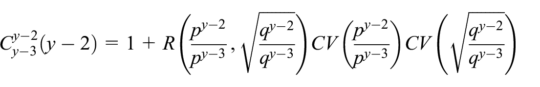
which means that it would in most cases be expected to be smaller than one. A similar interpretation can also be made for

and thus describes the ratio of a Walsh and a Paashe index. It has the alternative expression
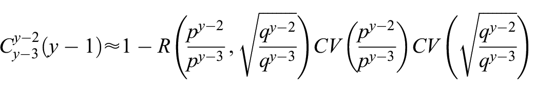
and we would usually expect for it to be larger than one, and hence, to affect rates of change upwards.
The total year-on-year reweighting effect of the CPI approach, which is a function of A, B, and C-type sub-components, can often be difficult to interpret. However, we have seen in this section that in certain cases, the C component as well as to some extent the joint effect of the A and B components, can be given bias correction interpretations. Next, we turn to the simulation study. As part of this study, we will also evaluate the sub-component decompositions derived in this section numerically on the Swedish data.
4. Simulation Study
4.1. Experimental Data
The simulation study was conducted on an experimental dataset constructed from CPI and National Accounts data from Statistics Sweden. The dataset included monthly so-called “basic” price indices and quarterly expenditures for all months of the period 2004 to 2023. (Although all aggregation methods listed in Table 1 are based on yearly quantities, quarterly values were needed to compile the year-on-year benchmark, to be specified below.) All in all, the data covered a basket of 395 CPI products (EPGs), divided into 118 National Accounts aggregates.
The basic price indices measure price change between December of the previous year and the current month, for a particular EPG. These indices were retrieved from the CPI database. For simplicity, only non-revised indices were included in the dataset, although in production, Statistics Sweden performs revisions at this level. (These revisions are incorporated into both short- and long-term links of the Swedish CPI and also affect HICP weights via the price updating procedures; see e.g., Bäcklund and Sammar 2012; Statistics Sweden 2025.)
Expenditure values were in turn obtained by combining CPI weight data, available at EPG level and on a yearly basis, with quarterly household expenditure information from the National Accounts, available at NA aggregate level. For year 2023, an approximation had to be used since data for this year had not yet been processed (i.e., allocated between EPGs) by the CPI production team at the time of conducting the study. Compared to actual production, another simplification was that a single set of expenditure data was used for each EPG and time period. (In production, different expenditure sets are employed for the compilation of short- and long-term weights, and these often differ because of revisions in the National Accounts and when updated external information has become available to the CPI team.)
Finally, to simplify the practical computations, values for EPGs which had been either introduced or removed from the Swedish CPI basket during the period under study were imputed in the experimental dataset. Basic price indices were imputed based on the price development of similar products, and expenditure values were set equal to 0.005% of the total basket value.
4.2. Simulation Setup
To compile the different index links of Table 1 (and Appendix A), all formulas were first rewritten as weighted sums of product level price relatives, and then implemented via EPG-level indices and weights. The EPG-level indices needed for this process were obtained by multiplying, or “chaining,” basic price indices. (This corresponds to how short- and long-term links of the Swedish CPI are compiled in practice; see e.g., Bäcklund and Sammar 2012.) Yearly and quarterly price indices were computed as the arithmetic average of the corresponding monthly values. The different kinds of weights needed for the compilations were finally derived via either directly or indirectly calculated price re-dated expenditure values.
Chained index series with start year r = 2005,
To evaluate the year-on-year results obtained from the different methods, a comparison was made with a “Fisher-like” benchmark formula. This benchmark was based on direct comparisons between current period prices and prices in the same month one year ago, which means that it does not include any “reweighting effects” in itself. Moreover, to avoid issues with seasonality, it was constructed from a basket representing twelve months of data. (As a remark, we note that using a full year of data for the basket also seems to be in line with the purpose of the Swedish CPI; the 1999 commission stated that “[the CPI] is essentially an annual index [… and …] aims to describe how the cost of an annual consumption […] develops over time”; SOU 1999, 63, authors translation; see also SOU 1999, 198, 206.)
Using
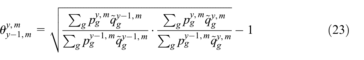
The hybrid quantities used in Equation (23) describe a kind of centralized yearly values. To define them in more detail, let

where c is a constant set to
In the simulation, comparisons between year-on-year inflation rates compiled according to the different methods, and the benchmark formula, were summarized in the form of three overall measures; a Root Mean Squared Error (RMSE), an Average Error (AV), and a Maximum Absolute Error (MAX). Letting
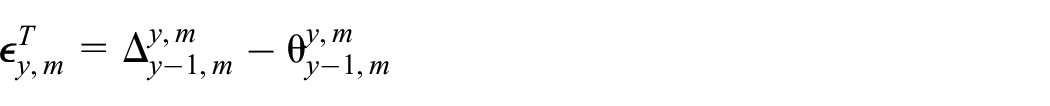
we can write these three summary measures as:
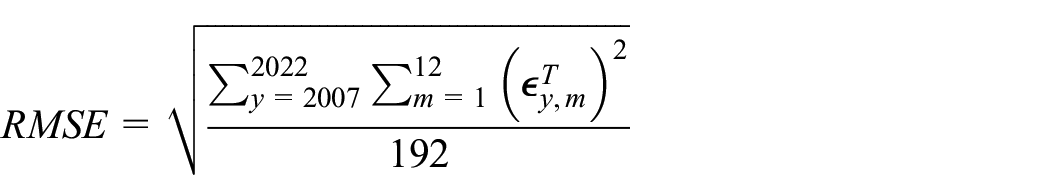
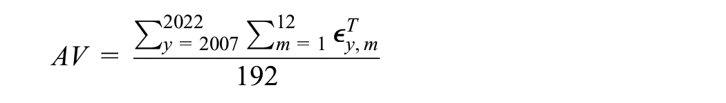
and
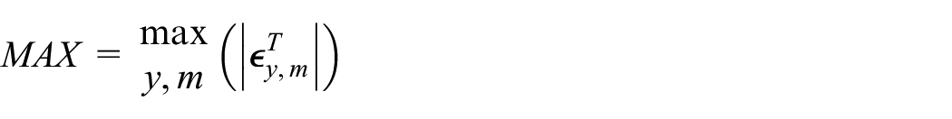
In the following, we will refer to
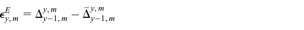
and a “formula error”, representing the effects of the choice of index formula and chaining strategy:
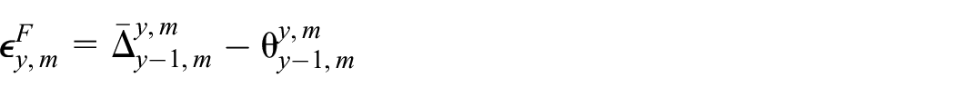
The estimation error is important to evaluate, since there is likely to be a trade-off between using the most up-to-date or the most reliable information to compile the short-term weights. However, it should be noted that this error will depend on the estimation method used to compile the indirectly calculated quantities—something which has not been a main focus in this paper. The formula error, on the other hand, measures the purely formula related aspects of each method and is thus directly related to the discussions of Section 3. In particular, we can use Equation (21) to rewrite it as the sum of the difference between the pure-price effect and the benchmark formula, and the reweighting effect:

While the first part of Equation (24) describes the effect of the choice of short-term basket on the formula error, the second part describes the joint effect of all other aspects of the higher-level aggregation method.
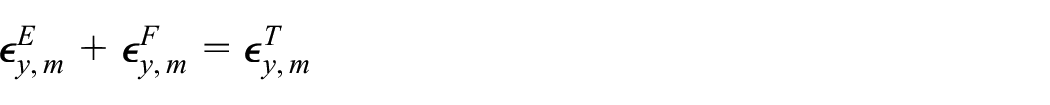
Obviously, the sum of the estimation and formula error in each time period is the total error:
Next, we report on the main results of the simulation study.
5. Numerical Results
5.1. Index Level Comparisons
To start with, we consider the effect that the choice of higher-level aggregation method has on long run index level results. Figure 1 shows a comparison between the average index values in year 2023 for series compiled according to the seven different methods. (Note that comparability is slightly hampered by the differing treatment of the first years of the series; Appendix A.) In squared brackets, we have also included corresponding values obtained from calculations based on only directly calculated quantities.
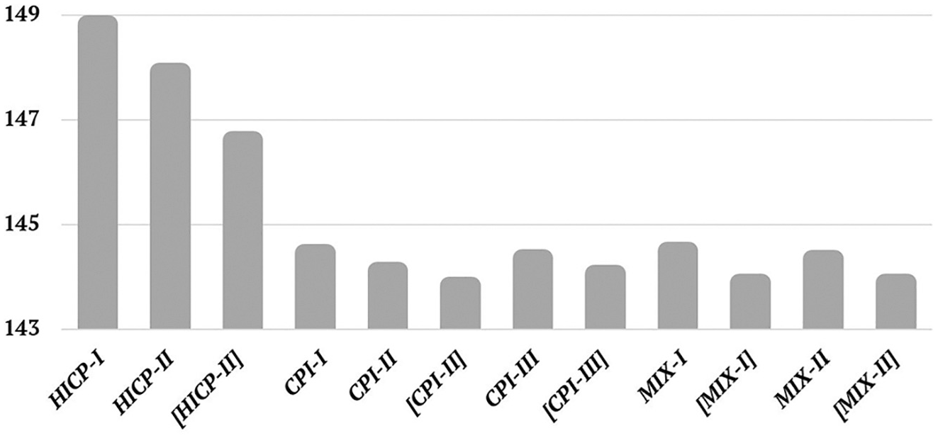
Average index values in 2023 (2005 = 100) for chained price indices compiled according to the different higher-level aggregation methods. In squared brackets are corresponding results compiled with indirectly calculated quantities replaced by directly calculated ones.
The highest index value (148.8) is obtained for method HICP-I, and the lowest (144.1) for CPI-II. All long-term link methods, however, give similar results. Overall, the use of long-term links leads to lower index levels over time. Detailed analysis also reveals that the difference between the long-term link approaches and the HICP approach is increasing fairly steadily over the research period, although increases are smaller in periods of low inflation.
For the HICP approach, using basket year y−1 instead of y−2 lowers the index level and reduces the gap to the long-term link methods. This result is consistent with previous studies showing that more recent weights in a Lowe index often gives rise to lower index levels and produces results which come closer to superlative indices. (See Greenlees and Williams 2009, Huang et al. 2017, and Walschots 2019.) Moreover, when the indirectly calculated quantities are replaced by direct ones, the index level decreases further. This result can probably be explained by the fact that the indirect estimates do not account for consumption shifts occurring within the same National Accounts aggregate. Even with directly calculated y−1 values in the short-term links, however, the HICP approach still gives rise to a higher average index than the long-term link approaches.
For users of the Swedish CPI, it is also interesting to compare the results of CPI-I to that of HICP-I, as well as CPI-II to HICP-II. These comparisons give indications on how the Swedish CPI would have behaved if the HICP aggregation approach had been used for the compilations instead of the current methodology. (For the period up to 2020, the first comparison is most relevant, while the second one is most relevant for the last three years.) In Figure 1, the difference between methods HICP-I and CPI-I is 4.4 index points, and that between HICP-II and CPI-II 3.8 points, corresponding to 3.0% and 2.6% higher index levels, respectively. According to this experiment, the Swedish CPI would thus have increased by somewhere between 2.6% and 3.0% more from 2005 to 2023, had the HICP methodology been used to compile the index, all other things being equal.
5.2. Year-on-Year Inflation Rates
Turning to year-on-year inflation, Table 3 shows overall results from the comparison between inflation rates compiled according to the different aggregation methods, and the benchmark formula. Judging by the total error RMSE, MIX-I performs best. This aggregation method even seems to have a small robustness advantage, since its maximum total error is also smallest. The other long-term link variations perform quite similarly but their differences with respect to HICP-II is smaller. In particular, this is the case for CPI-II, which also has a larger maximum error than HICP-II. Although CPI-II performs on average slightly better than HICP-II, it thus also gives rise to larger errors in specific time periods.
Simulation Results for Year-on-Year Rates of Change for the Period 2007 to 2022. All Values Have Been Multiplied by 100.
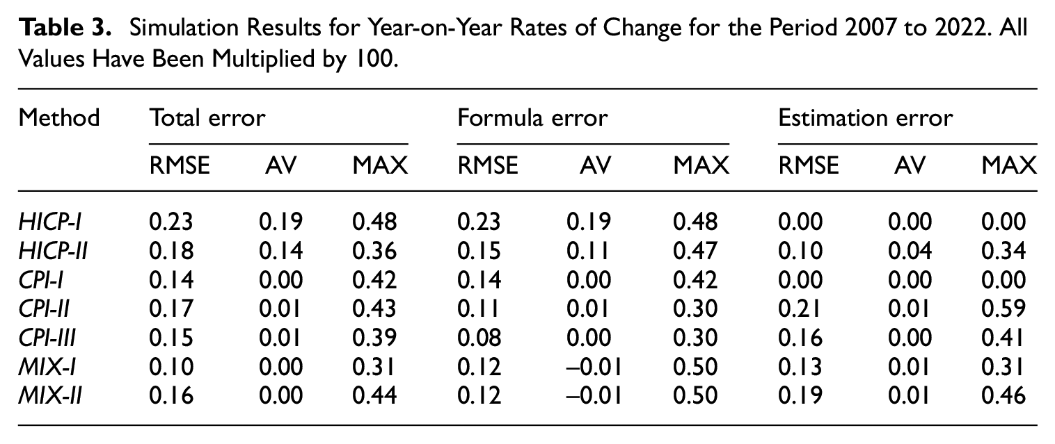
In contrast to HICP-I and HICP-II, the long-term link approaches all have total errors which are to a large extent “random” over time. In other words, their average total errors over the whole period are small. For example, CPI-I and CPI-II give rise to average errors of 0.00 and 0.01 percentage points, respectively, whereas the corresponding values for HICP-I and HICP-II are 0.19 and 0.14 percentage points. (These numbers also imply that the average difference in year-on-year inflation between CPI-I and HICP-I is approximately 0.19 percentage points, and that between CPI-II and HICP-II approximately 0.13 points. In other words, if basket year y−2 is used in the compilation of short-term links, year-on-year rates of change are approximately 0.2 percentage points lower for the current CPI approach than for the HICP approach, while they are approximately 0.1 percentage points lower if an approximate y−1 basket is used.) For the MIX approach, the average error is 0.00 percentage points for both variations.
Looking more closely at the estimation error, we note that this error is most important for the long-term link methods (except, of course, for CPI-I). The average estimation error is, however, small for all methods, indicating no clear systematic over- or under estimation. Hence, the fact that the indirectly calculated quantities gave rise to higher index values in Figure 1 does not seem to carry over to systematic effects on year-on-year rates of change. Interestingly, MIX-I has a smaller estimation error than MIX-II, despite being based only on indirectly calculated quantities. This might indicate that it is advantageous to use the same kind of quantity estimates—that is, either indirect or direct ones—in the numerator and denominator of the inflation rate computations. Another interesting observation is that for the current CPI approach, the increase in estimation error when going from method CPI-I to CPI-II more than outweighs the decrease in formula error. This result implies that it might actually have been more favorable for Statistics Sweden to use y−2 quantities for the CPI short-term links in 2021 to 2024 than to use the y−1 approximation. (On the other hand, users also value consistency between the different measures of inflation and using different basket years for the CPI and HICP would have meant different within-year patterns for the two indices.)
As expected, the formula error is instead most important for the HICP approach. Judging by the RMSE, method CPI-III performed best in this respect. The other long-term link methods based on basket year y−1, that is, CPI-II, MIX-I, and MIX-II, also give similar results. In particular, CPI-II comes close to CPI-III both in terms of RMSE and maximum error.
For the HICP approach, using basket year y−1 instead of y−2 decreases the formula error. More detailed analysis reveals that this is actually the case in all years except for in 2021. During 2021, however, the formula error is larger for HICP-II than for HICP-I in most months. This is an interesting result given that the methodological change from basket year y−2 to y−1 in the HICP was introduced precisely in this year. A similar pattern can also be seen for the CPI approach, where CPI-I has a smaller formula error than CPI-II for most of 2021, but also in 2010 and 2011.
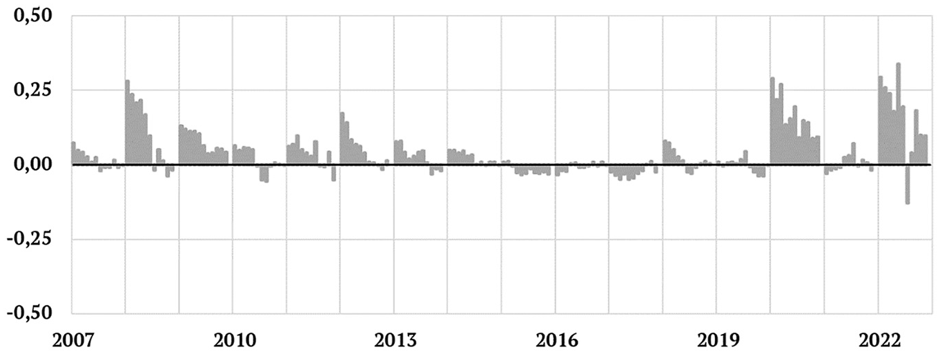
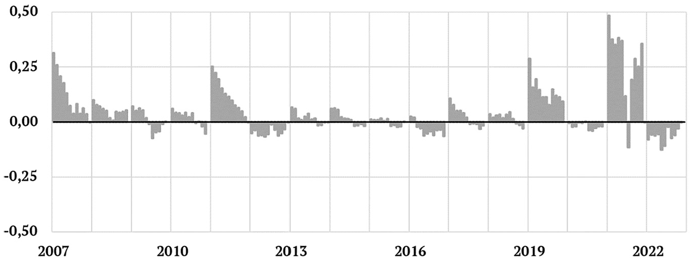
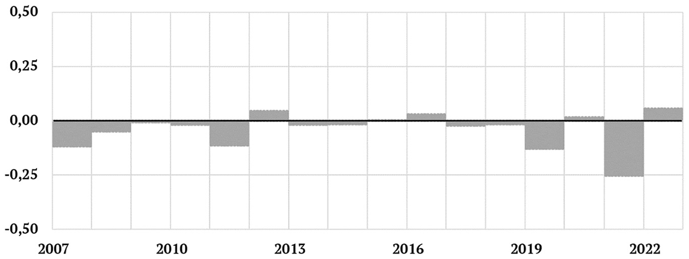
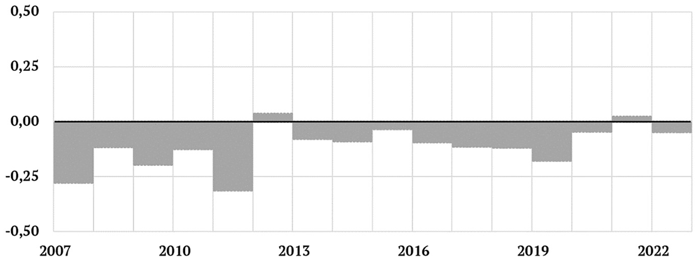
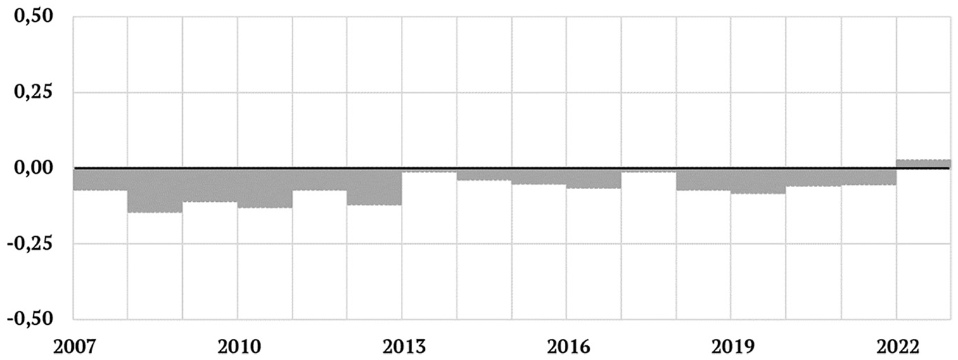
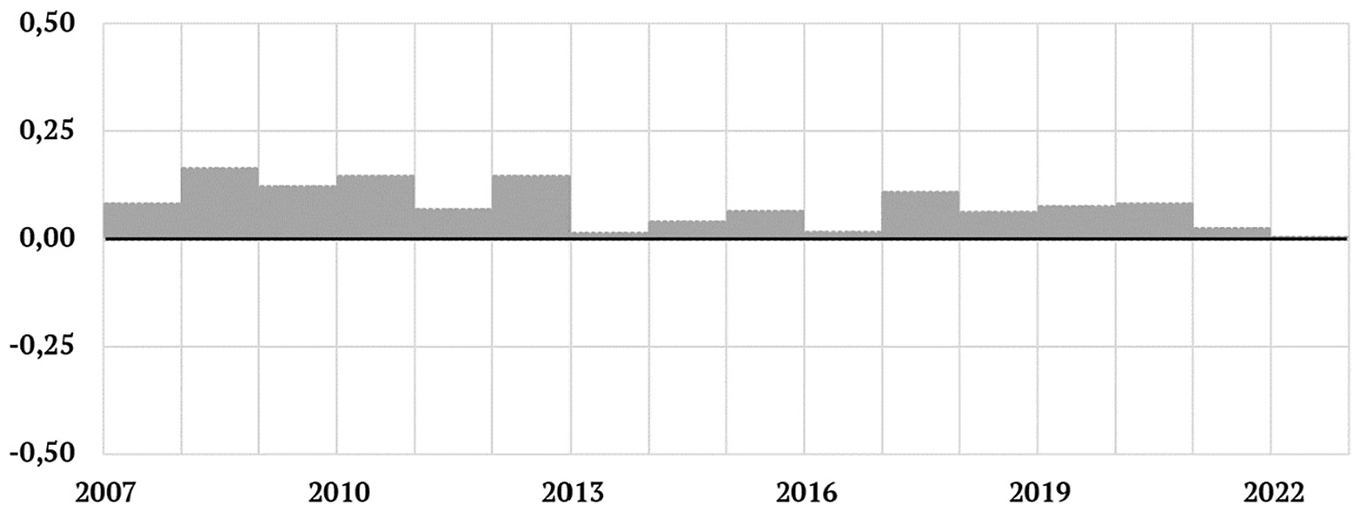
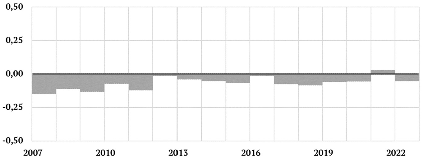
In Figures 2 and 3, we further consider the decomposition of the formula error into its pure-price and reweighting parts; cf. Equation (24). Figure 2 shows the difference between the pure-price effect and the benchmark formula, and Figure 3 the total reweighting effect. From Figure 2, we can note that the pure-price part of the formula error is mostly positive, and increasing over the year (as the benchmark basket gets increasingly distant from year b). It is also clear that using a more recent short-term basket decreases the pure-price part of the formula error. Over the whole period, the average difference between
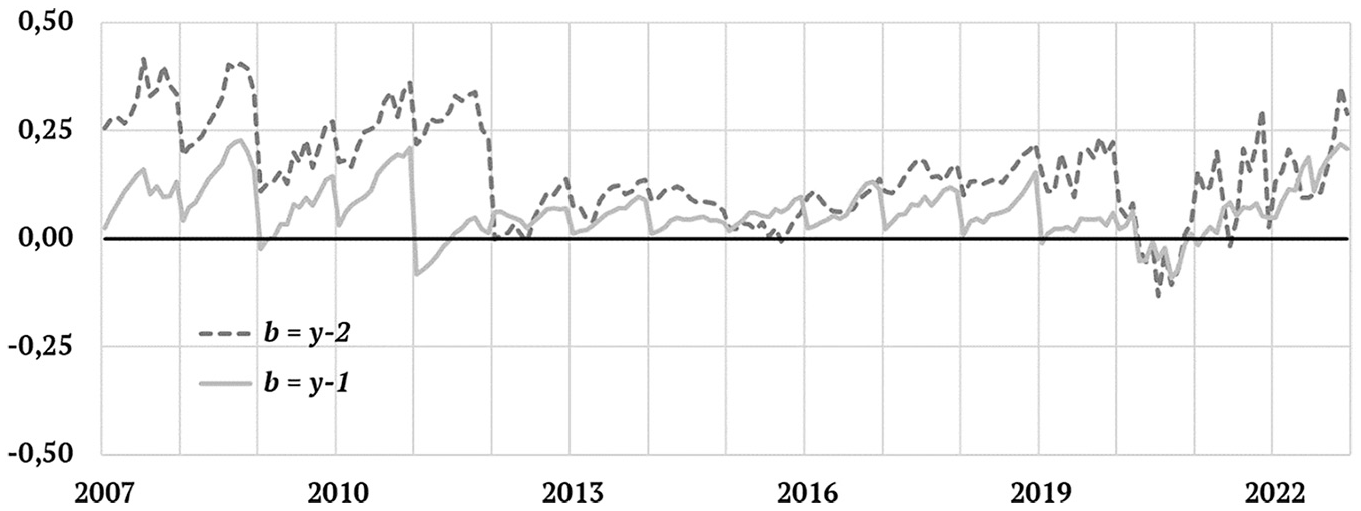
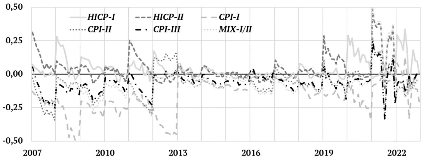
In general, to obtain a small formula error, we would ideally want Figure 3 to show the inverse pattern compared to Figure 2. In other words, we would want the reweighting effects to be slightly negative and decreasing over the year. At least in some periods, Figure 3 indicates that the long-term link approaches are slightly more in line with this scenario than the HICP approach.
It is also possible to digest the formula error further by plotting the reweighting sub-components derived in Section 3. This is done in Figures 4 to 12. Most of these figures show more or less the expected pattern in terms of negative or positive contributions to the total reweighting effects, but certain results stand out. Interestingly, some of these can be interpreted as Covid-19 related effects. For example, the sub-component
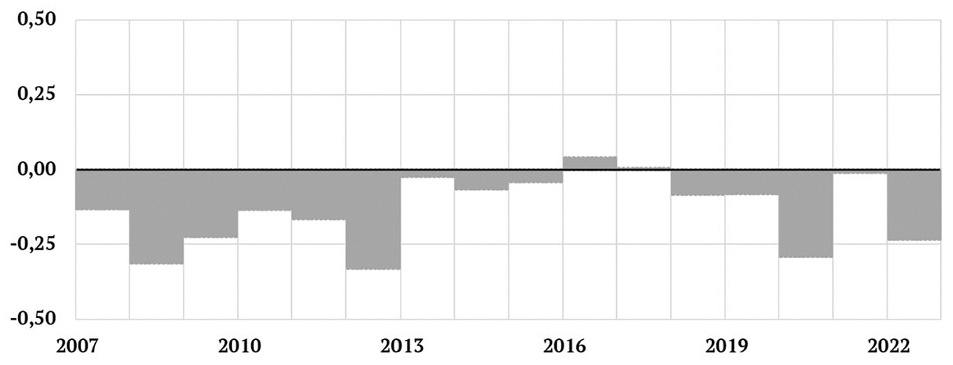
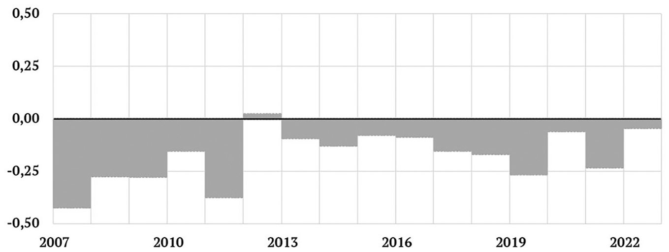
Many of the larger variations seen in the sub-component plots can also, after more detailed analysis, be explained by changes in the National Accounts compilation practices. (Because of the non-revision policy of the CPI, such adjustments can have large one-time effects on CPI weights.)
6. Final Remarks
In this paper, we have compared the higher-level aggregation approaches of the Swedish Consumer Price Index to that of the European Harmonized Index of Consumer Prices. Assuming a superlative index as the operational target parameter, the Swedish methods have an advantage over the HICP approach for long run price comparisons. For month-on-month and year-on-year rates of change, however, things are less clear. In this paper, we used Swedish data to compare year-on-year inflation rates compiled according to the different methods to a superlative-like benchmark formula. Results indicated that the Swedish methods work well also for year-on-year rates of change, with the largest gains obtained when short-term weights are based on two-year-old data. Future research could be devoted to evaluating also the mixed approach under alternative setups for the short-term weights.
For practical reasons, certain aspects were left out of this study. For example, the evaluations should ideally have taken statistical uncertainties in the underlying price and expenditure data into account. (Although Statistics Sweden has done some research on variance estimation for the CPI–most recently, Norberg and Tongur 2022–more work is needed before those estimates can be applied to this kind of investigation.) Other index formulas could also have been tested for the different links. For example, several countries make use of Young, rather than Lowe, indices in their CPIs (see e.g., Hansen 2007), and more complex alternatives such as the ones explored by Armknecht and Silver (2014) could also have been included. Some of these were, however, already considered in the Swedish CPI context by the 1999 commission.
Another aspect which would be worth investigating further is the effect of revisions to the price and quantity data. Clearly, the use of long-term links opens the possibility to implicitly revise not only weights, but also indices. Biases at lower levels of the CPI can thus potentially be addressed via a long-term link methodology. In particular, superlative bilateral indices or fully transitive multilateral formulas could replace the original basic indices in the compilation of long-term links. This kind of revision possibility is only partially exploited in Statistics Sweden’s production today. Revisions to the National Accounts could also be accounted for with time. Specifically, the medium-term link idea described in this paper could be extended to incorporate several different sets of medium-term links, complied with different lags. This would enable more final National Accounts data, and even benchmark revisions, to be introduced into the non-revisable index series after several years. (See Herzberg et al. 2022, for an analysis of the effect of using final NA data to compile weights for the HICP.) Moreover, the long-term links could also be used to introduce special one-time adjustments. For example, the possibility of modifying the long-term links to control for weight-related effects of the Covid-19 pandemic was discussed by Statistics Sweden (see e.g., Ståhl 2023b). The main idea—which was, however, never implemented—was to replace part of the long-term chain by a direct link running from 2019 to 2022. This would have prevented pandemic-related weight effects from influencing the long run level of the CPI series altogether. Of course, such a special adjustment could also have been used to retroactively incorporate revised (possibly imputed) price data into the index. (For more on the difficulties associated with imputing missing prices in the CPI during the Covid-19 pandemic, see Abe 2022; Boldsen 2022; Diewert and Fox 2022a, 2022b; Goldhammer 2022.)
Finally, it should be noted that although our simulation indicated that overall, i.e., over the whole research period, the long-term link aggregation approaches worked well also for year-on-year rates of change, this is not certain to be the case in any given year. There is always the risk of the implicit revisions distorting inflation rates. For some users, it could therefore be valuable to have access to a retroactively compiled monthly analytic index which is consistent with the development of the long-term chain of the CPI—in other words, a series where long-term link effects have been incorporated into the “correct” year. This would require the compilation of some form of revised short-term links, somehow benchmarked against the long-term chain. Practical methods such as the ones recently proposed by von Auer and Shumskikh (2024) could potentially be useful for this aim. We consider this an interesting topic for future research.
Footnotes
Appendix A
Appendix B
Appendix C
Acknowledgements
I wish to thank the Editor, the Associate Editor, and an anonymous referee for providing comments and suggestions which helped significantly improve the quality of the paper. Emanuel Carlsson and Can Tongur offered valuable feedback on an earlier draft. This research was previously presented at the 18th meeting of the Ottawa Group on Price Indices in Ottawa, Canada, 13–15 May 2024, and I also wish to thank Erwin Diewert and the other participants of this meeting for their helpful comments and suggestions. Finally, please note that all views expressed in the paper are those of the author and that they do not necessarily reflect the views of Statistics Sweden.
Funding
The author received no financial support for the research, authorship, and/or publication of this article.
Received: May 24, 2024
Accepted: March 12, 2025