
Abstract
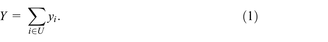
Usually, Statistical Institutes and Research Centers present the results of surveys in a “standardized” way, that is, the estimator of the parameter of interest and the associated measure of accuracy. This implies the calculation of the variance of the estimator, which is typically done in two possible ways: analytically or with replication methods. The analytic way requires the availability of the information of auxiliary variables used in the methodological plan of the survey, both at the sample level for the design variables, and at the respondent level for the variables involved in the treatment of non-response. Unfortunately, these variables are often not available in the final survey dataset, and the variance might therefore be miscalculated. Replication methods, which fully integrate the methodological plan applied into the survey, may be considered as good alternatives to this approach. This paper uses real data from the survey on “Racism and Ethno-racial Discrimination” carried out in Luxembourg in 2021, to compute and compare analytic variance estimators and bootstrap variance estimators. For this survey, both the linearization and the rescaled bootstrap lead to similar results, but the ultimate cluster variance estimator can be substantially biased. This suggests that the rescaled bootstrap may be a relevant approach.
1. Introduction
The analysis of complex survey data usually requires the computation of confidence intervals (and therefore, of the variance) of the estimator for an accurate interpretation of the results, that is, the survey error. An error on their calculation can lead to a misinterpretation of the results (J. N. K. Rao 2016). However, in practice, these calculations become tedious, specially from an user perspective. The set of weights needed for their computation is generally obtained from a combination of different statistical procedures, which the user rarely has access to. In the simplest cases, these statistical procedures include sampling, correction for unit non-response, and the final calibration step. Each of the mentioned procedures (or steps) has its own random component, that should be taken into account when calculating the confidence interval of each estimator. The literature distinguishes between two approaches to compute confidence intervals and/or variance estimators: (1) the analytical approach, which is typically associated to linearization techniques for the non-linear estimators, and (2) resampling methods as an alternative.
The analytical approach requires a perfect knowledge on the survey process (sampling and estimation) to compute the variance. If we consider the process described above (sampling, correction for unit non-response, calibration), we first compute the sampling variance, which depends on the sampling plan. Secondly, we account for the variance due to unit non-response, usually by assimilating unit non-response to an additional sampling phase, see Särndal and Swensson (1987) and Caron (1998) for the resulting formulas for an easier implementation. The so-called “reverse approach” (e.g., Beaumont and Haziza 2016) enables a simplification of the formulas from Särndal and Swensson (1987). Thirdly, we account for the calibration of weights. Finally, the linearization approach (J.-C. Deville 1999) can be used to perform variance estimation for non-linear parameters.
Resampling methods such as Jackknife (Quenouille 1956; Tukey 1958), balanced repeated replication (McCarthy 1969), and bootstrap (Efron 1979) are seen as good substitutes for the analytical methods. In resampling methods, “artificial” samples are drawn from the initial sample. Each of these samples is used to create a replicated version of the original estimator, after correction for unit non-response and calibration. The sequence of replicated weights is used to obtain a simulation-based variance estimator, and then to obtain confidence intervals. We focus here on bootstrap methods, which were initially proposed for independent and identically distributed (i.i.d.) data (Efron 1979). The adaptation to survey data on finite populations has been the topic of a substantial literature, see for example Chauvet (2007), Mashreghi et al. (2016), and the references therein. Among the bootstrap methods proposed for survey sampling, the most used is the rescaled bootstrap of Rao and Wu (1988). It consists in producing bootstrap resamples by means of a basic bootstrap strategy, and then to rescale the resampled values to match an unbiased variance estimator. A modification is proposed in Rao et al. (1992), where the rescaling is applied to the sampling weights. A particular choice of the resampling size leads to the usual with-replacement bootstrap as a particular case. The rescaled bootstrap is generally accurate for sampling designs with a small first-stage sampling fraction, and is conservative otherwise. Beaumont and Émond (2022) recently proposed a unified bootstrap method which may be applied either to multistage sampling designs or to two-phase sampling designs with Poisson sampling at the second phase, without the assumption of a small sampling fraction at the first stage. In the rest of the article, we use the rescaled bootstrap algorithm in Rao et al. (1992). The correction for unit non-response and calibration are integrated in a similar way as in Bessonneau et al. (2021), to obtain a set of bootstrap weights at the level of the survey units.
The aim of this article is to study and compare the variance estimators and confidence intervals obtained under both the linearization approach and the bootstrap approach, in an application with real data from the survey on “Racism and Ethno-racial Discrimination” carried out in Luxembourg in 2021. This survey has two particularities. Firstly, the sampling fraction varies between 1.6% and 10.3% inside strata. It is therefore not negligible in some strata, in which the variance could be overestimated by the bootstrap. Secondly, the response rate is quite low, below 20%, which means that the variance due to unit non-response may be a large part of the overall variance. Our empirical results enable us to confirm on real survey data that both the linearization approach and the rescaled bootstrap approach lead to very similar variance estimates.
The rest of the article is organized as follows. We describe in Section 2 how to estimate the variance of an expansion estimator. We first consider in Subsection 2.1 an analytical approach, and the way by which the different sampling and estimation steps are dealt with in variance estimation. In Subsection 2.2, we explain how the rescaled bootstrap is applied in our case, and compare the bootstrap variance estimators with analytic variance estimators. In Section 3, the sampling design of the survey “Racism and Ethno-racial Discrimination” is described. The results obtained when comparing both approaches are presented and discussed in Subsection 4. The sample from this survey is used to build a pseudo-population, on which we perform a simulation study. The results are presented in Subsection 4.1. Finally, Section 5 summarizes our main conclusions.
2. Methodology
We consider a classical sampling design for a survey of individuals, in a population for which a sampling frame is available. Apart from the definition and the building of the sampling frame, three main steps need to be accounted for in estimation, namely (1) sample selection, (2) correction of unit non-response, and (3) calibration of the survey weights.
2.1. Analytical Variance
2.1.1. Sampling Design
Let
Let
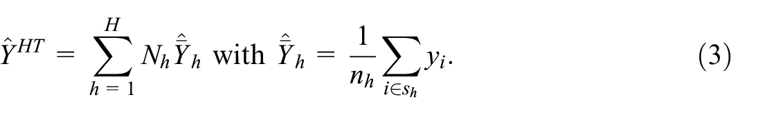
The general formula for the Horvitz-Thompson estimator (Horvitz and Thompson 1952) is
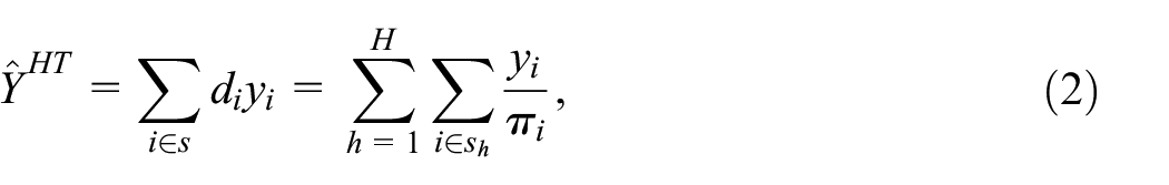
where
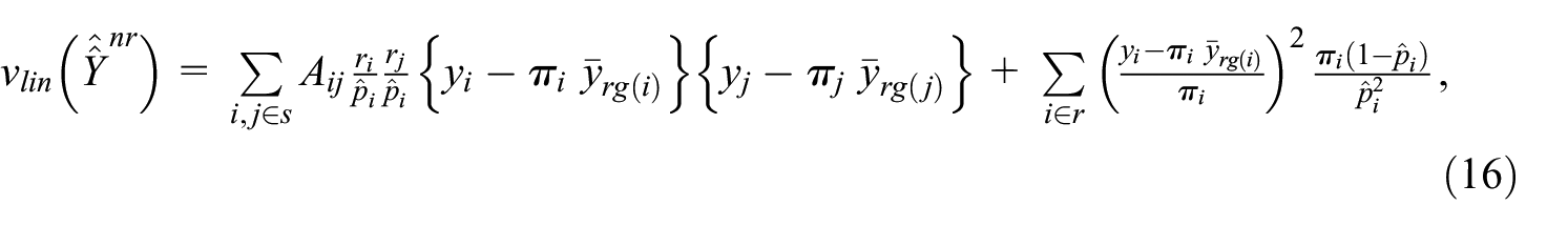
Under stratified simple random sampling without replacement, the Horvitz-Thompson estimator simplifies as
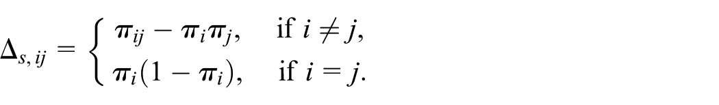
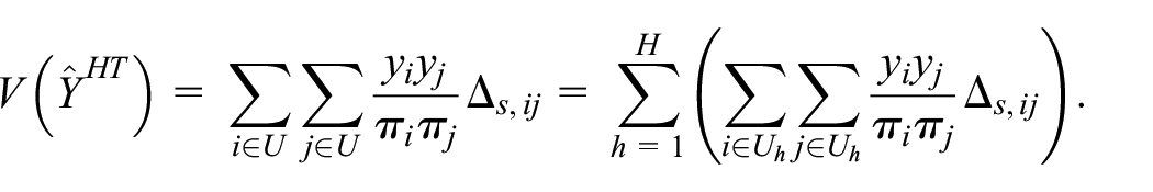
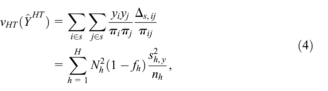
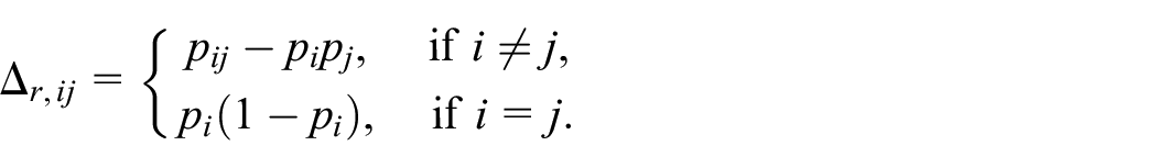
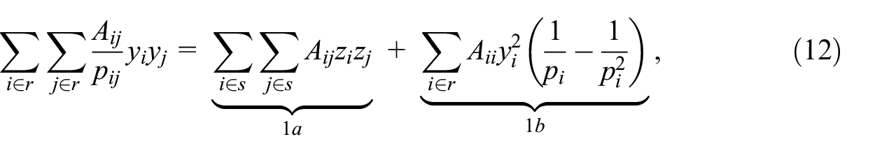
An unbiased estimator of variance is given by
where
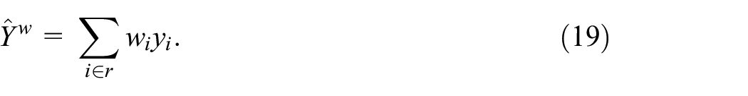
2.1.2. Non-Response Correction
In survey sampling, unit non-response is usually treated as a supplementary sampling phase (see Särndal and Swensson 1987). This approach allows to consider, in a simple way, the correction for non-response in the calculation of an estimator and in the estimation of its variance. In this section, we explain how to obtain the estimator of the variance of a total of a variable of interest after the correction of unit non-response.
Under unit non-response, we suppose that an additional phase is added in the sampling process, which may be described as follows. From the realization of the sample

We also use the notation

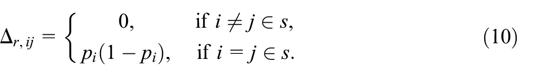
We suppose that the response probabilities
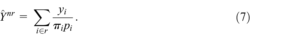
We first suppose that the response probabilities are known. In such case, an expansion estimator is
Following Särndal and Swensson (1987), the associated variance of this estimator is given by
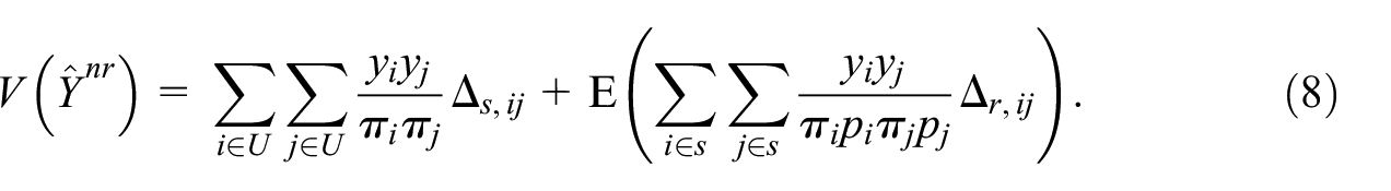
The interpretation of the formula is simple: the variance of an estimator under two-phase sampling is given by the sum of the variance of the first sampling phase (first term in the right-hand side of Equation (8)) and the variance of the second sampling phase (second term in the right-hand side of Equation (8)). An unbiased estimator of the variance proposed also by Särndal and Swensson (1987) is given by
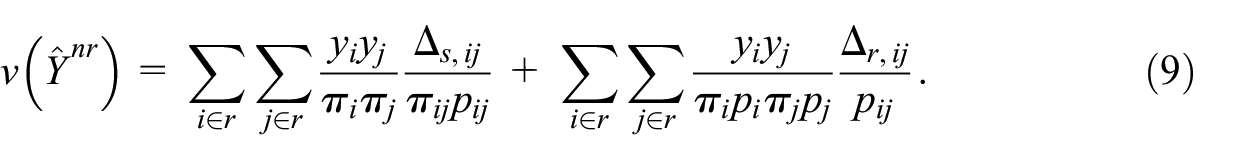
In practice, even with a simple survey procedure as the one presented in this paper, the Equation (9) is not straightforward to program. It involves several multiple sums, at the level of the first phase, of the second phase, and also between phases. Caron (1998) proposed variance estimation formulas in the specific cases when Poisson sampling or stratified simple random sampling without replacement is used at the second phase. In this work, we focus on Poisson sampling at the second phase, since it is the one used to model unit non-response in our survey “Racism and discrimination ethno-racial” in Luxembourg (see Section 3).
Under Poisson sampling, the individuals in the sample
The variance estimator in Equation (9) may then be rewritten as
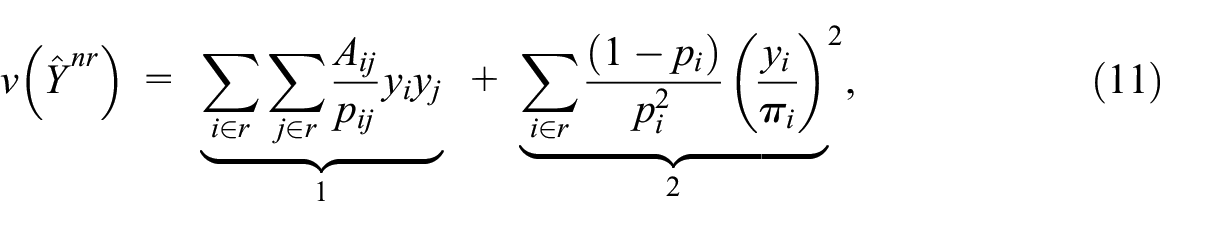
where
where
In practice, the response probabilities
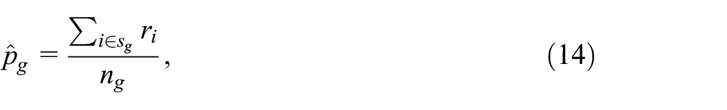
with
The estimator of the total accounting for the estimation of the response probabilities is
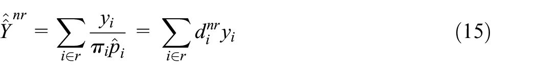
where
where
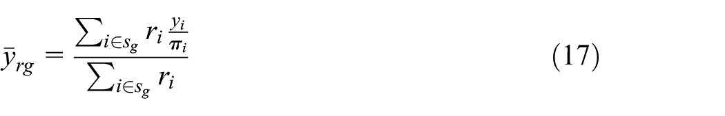
is the mean among respondents of the variable
2.1.3. Calibration
Normally, after the correction of non-response, it is common to include an additional step of calibration on totals of auxiliary variables known at the level of the population. The aim of calibration is to reduce the variance of the estimator of the total, which is the case if there is an (approximately) linear relationship between the variable of interest and the auxiliary variables.
Calibration methods require a vector of

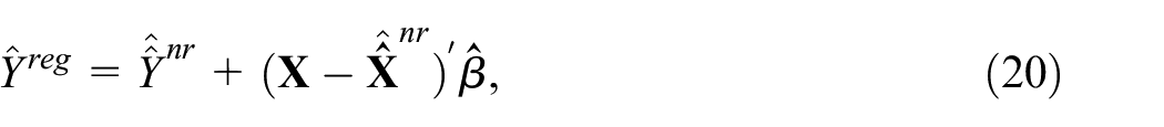
The calibration estimator of the total in (1) proposed by Deville and Särndal (1992) is given by:
Deville and Särndal (1992) showed that, under some mild conditions, the calibration estimator under any distance function is asymptotically equivalent to the generalized regression (GREG) estimator. Let
where
The asymptotic equivalence between the calibrated estimator and the generalized regression estimator implies that they share the same asymptotic variance, see Deville and Särndal (1992) for a proof.
For variance estimation, let

denote the estimated residuals in the weighted regression of the variable of interest
where
2.1.4. Extension for Other Parameters
If the population size
and the variance estimator
It is very common in statistical institutes to estimate other parameters, such as a ratio
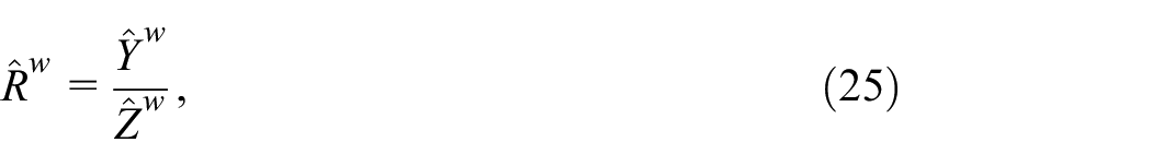
using a substitution principle. Since both the numerator and denominator in (25) are random variables, the calculation of the variance requires a previous step which is called linearization (e.g., Deville 1999; Woodruff 1971). The estimated linearized variable associated to the ratio
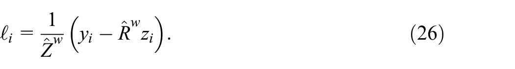
The estimated residuals
2.2. Bootstrap Variance
In practice, the computation of the variance estimator defined in Subsection 2.1 may not be easy. In particular, auxiliary design variables (the strata indicators) need to be available at the level of the sample
Resampling methods such as Jackknife (Quenouille 1956; Tukey 1958), balanced repeated replication (McCarthy 1969), and bootstrap (Efron 1979) are good alternatives to the calculations of analytic variance estimators. In this paper, we focus on the bootstrap method proposed by Rao and Wu (1988) and its generalization proposed in Rao et al. (1992). This technique has shown a very good performance in case of stratified multi stage sampling with a negligible first-stage sampling fraction, see Beaumont and Patak (2012), Beaumont and Émond (2022), Chen et al. (2022). This is also a well-established variance estimation method in many national statistical offices. The method proposed by Rao and Wu (1988) is reviewed in Subsection 2.2.1, and an adaptation accounting for unit non-response and calibration is presented in Algorithm 3. In Subsection 2.2.2, we give the benchmark analytic variance estimators that the bootstrap aims at reproducing in the linear case, and compare them to alternatives.
2.2.1. The Rescaled Bootstrap
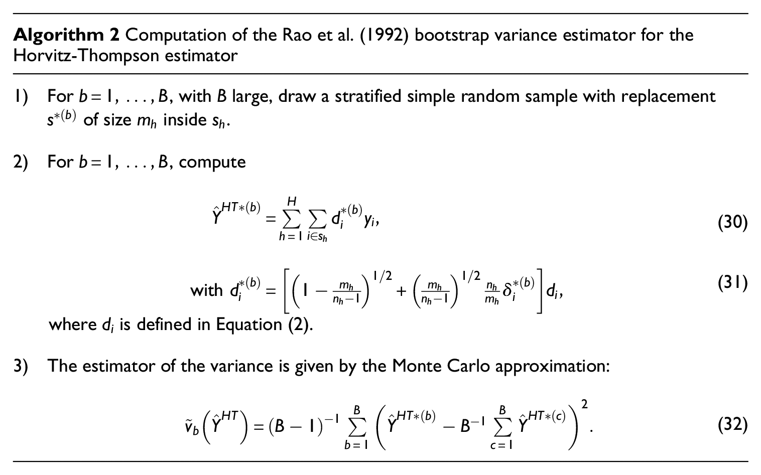
This bootstrap method proposed by Rao and Wu (1988) is suitable for multistage sampling designs, with a fixed-size sampling design at the first-stage, possibly stratified, which may be performed either with or without replacement. In line with Subsection 2.1, we consider the method in the particular case when the sample is selected by a one-stage sampling design, namely stratified simple random sampling without replacement. Following Rao and Wu (1988), a bootstrap variance estimator for the Horvitz-Thompson estimator may be computed as described in Algorithm 1.
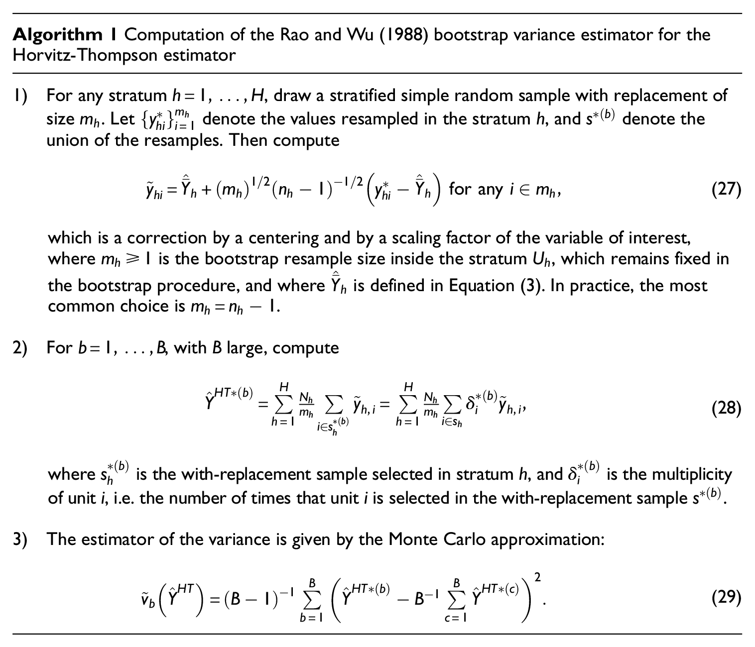
Since Step 1 in Algorithm 1 is specific to the variable of interest, the procedure should be repeated separately for each of them, which leads in a not efficient method computationally speaking. Rao et al. (1992) propose a modification of the procedure, where the centering/scaling correction is applied on the sampling weights rather than on the variable of interest. This leads to Algorithm 2. The resampling is done at the level of the sampling unit, provides better estimation of the sampling variance. However, we still need to integrate the non-response correction and calibration as described in Subsection 2.1.
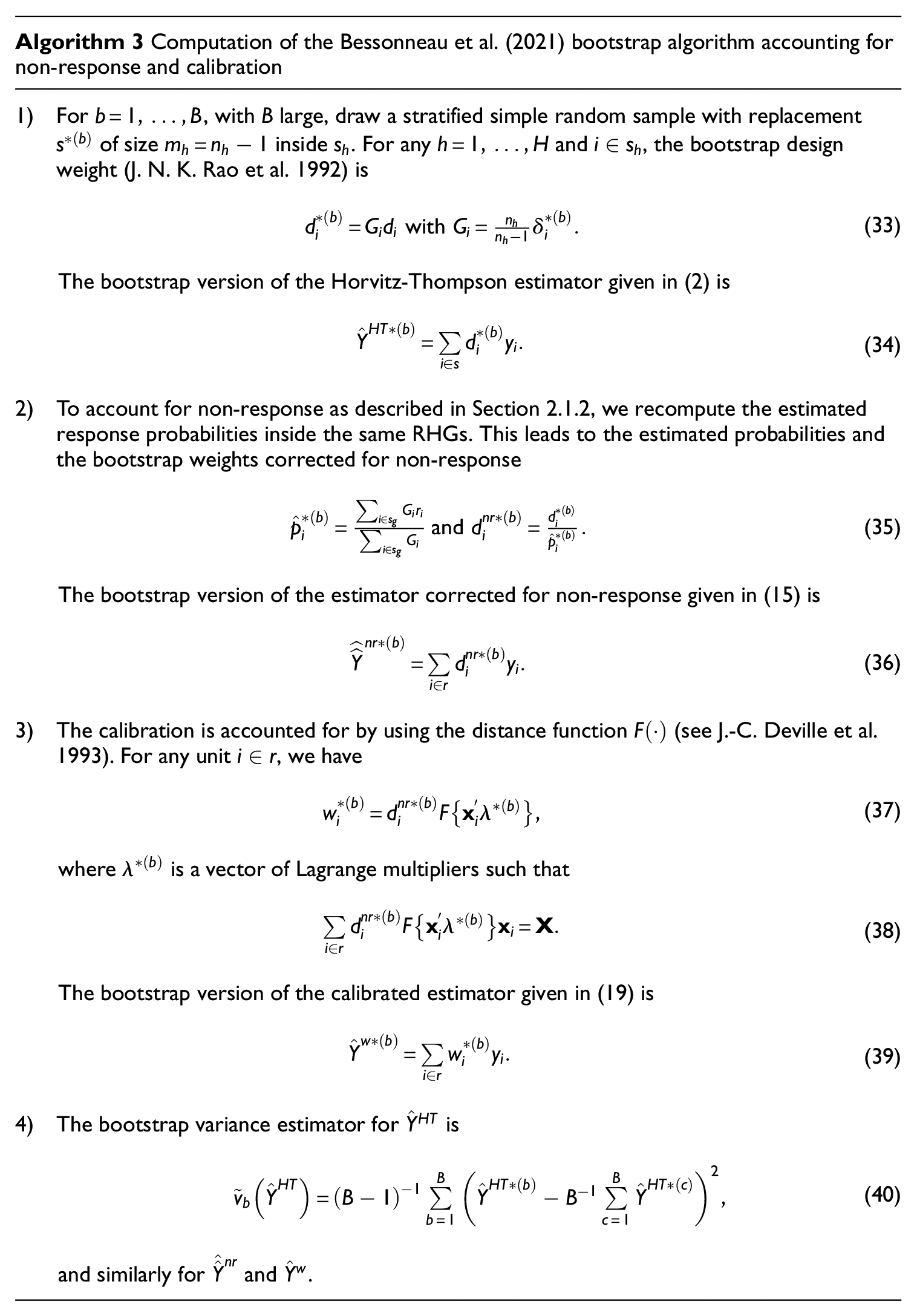
The bootstrap variance estimator given in Equation (32) accounts for the sampling error. Surveys are prone to other sources of variability, like unit non-response. Rust and Rao (1996) highlight the importance of computing accurately survey error including non-response error when estimating population parameters. They provide some practical examples of health surveys with multistage sampling designs, and design weights corrected for non-response and adjusted via post-stratification. They implemented and analyzed resampling techniques (Jackknife, balanced repeated replication, and bootstrap) in this context. Recently, Bessonneau et al. (2021) proposed two SAS macros including the procedure proposed by Rao et al. (1992) plus the two next steps, non-response correction and calibration. The first macro was designed to obtain the bootstrap replicate weights for single-stage sampling, while the second one was designed to obtain bootstrap replicate weights for two-stage sampling. Since our survey is single-stage, we focus on the algorithm beneath the first macro, which is described in Algorithm 3. Note that the response indicators
2.2.2. A Comparison Between Bootstrap Variance Estimators and Alternatives
In this section, we review the benchmark variance estimators for the bootstrap, that is, the analytic variance estimators that the bootstrap aims at matching for the estimation of a total (Bessonneau et al. 2021). We compare them with alternative analytic variance estimators.
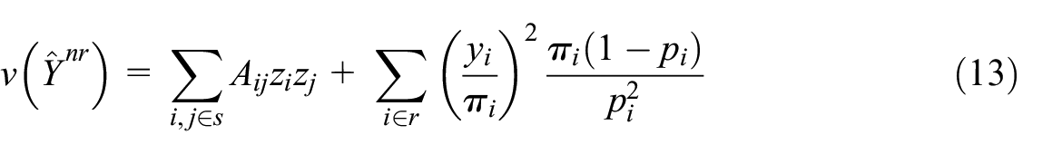
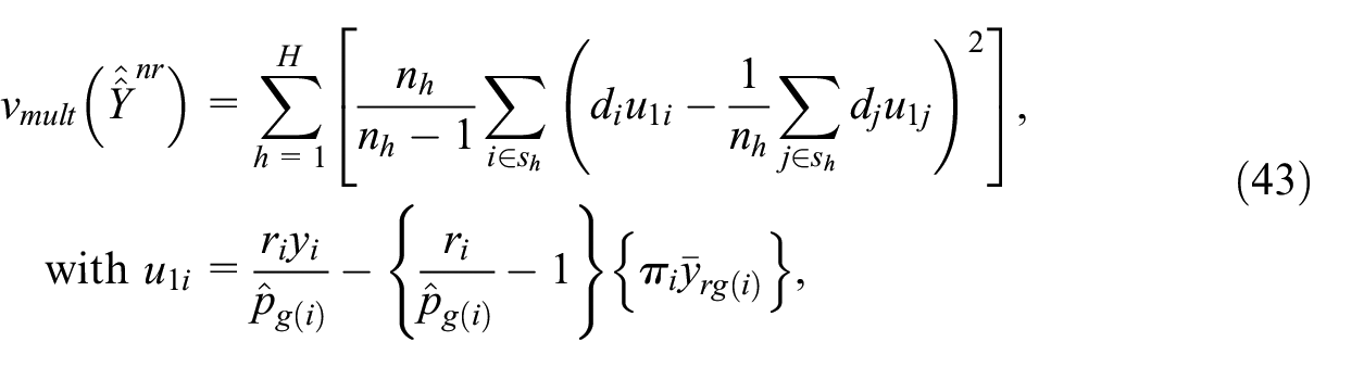
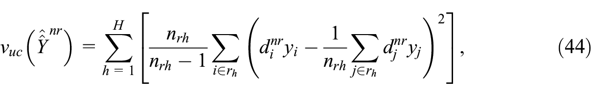
For the Horvitz-Thompson estimator, the benchmark variance estimator is
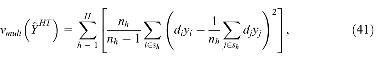
see Bessonneau et al. (2021, Equation 2.4). This is the unbiased variance estimator that would be used if the samples were selected with replacement inside strata. It is often called the ultimate cluster (UC) variance estimator. A more general form is
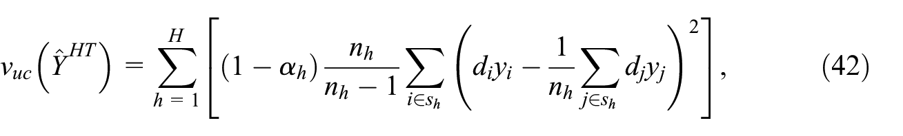
where
For the estimator corrected for unit non-response, the benchmark variance estimator is
and
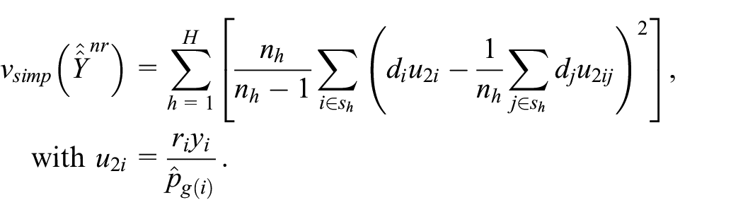
This amounts to estimating the variance as if the response probabilities were known rather than estimated. This usually results in an overestimation of the variance (Kim and Kim 2007), but the overestimation is expected to be limited if the sample size is sufficiently large inside each RHG. An alternative is the ultimate cluster variance estimator, computed on the respondent sample with the weights corrected for non-response:
with
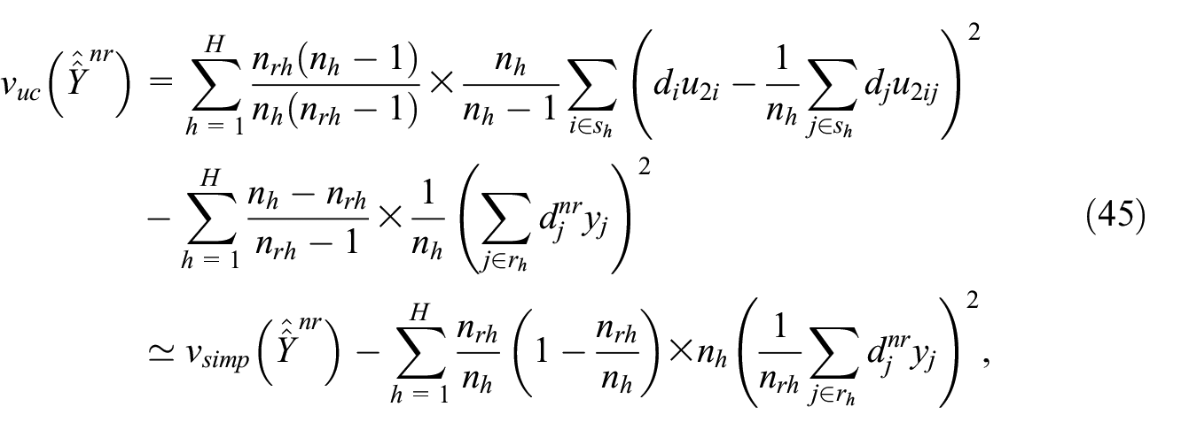
where the second (approximative) equality in Equation (45) holds if the number of respondents
For the calibrated estimator, the benchmark variance estimator is
and where
This variance estimator is asymptotically equivalent to
The ultimate cluster variance estimator is widespread among survey data users, due to its simplicity. It is included in statistical software like the procedure SURVEYMEANS of SAS®, with the possibility to perform a finite population correction at the first-stage inside strata (Valliant 2004).
3. Description of the Data
In this section, we describe an application with real data, in which we compare the results obtained with the analytic variance estimator and the bootstrap variance estimator. This application is based on the survey on “Racism and ethno-racial discrimination,” run by Luxembourg Institute of Socio-Economic Research (LISER) in 2021. A sample of 15,000 individuals of eighteen years and older have been chosen with a probabilistic sampling design to reply to an online questionnaire. This survey has been conducted between March and December 2021 and the conclusions have been presented in 2022. The main aim of the survey is to measure the perceptions of the residents in Luxembourg and of the minority groups, with respect to discrimination or racism in several aspects of daily life: employment, housing, health, education, relations with public administration, among others. Discrimination or racism is defined as distinctions and/or marginalization based on personal characteristics such as skin color, religion, country of birth or nationality, language accent, dressing, or cultural practices. Minority groups are defined with respect to the country of birth.
We begin with summarizing the methodological plan for the survey. It is divided in four parts: definition of the reference population or sampling frame, definition of the sampling design, choice of the (undesirable) non-response correction model, and choice of the final calibration model on margins. Further information can be found in Docquier et al. (2022).
3.1. Sampling Frame
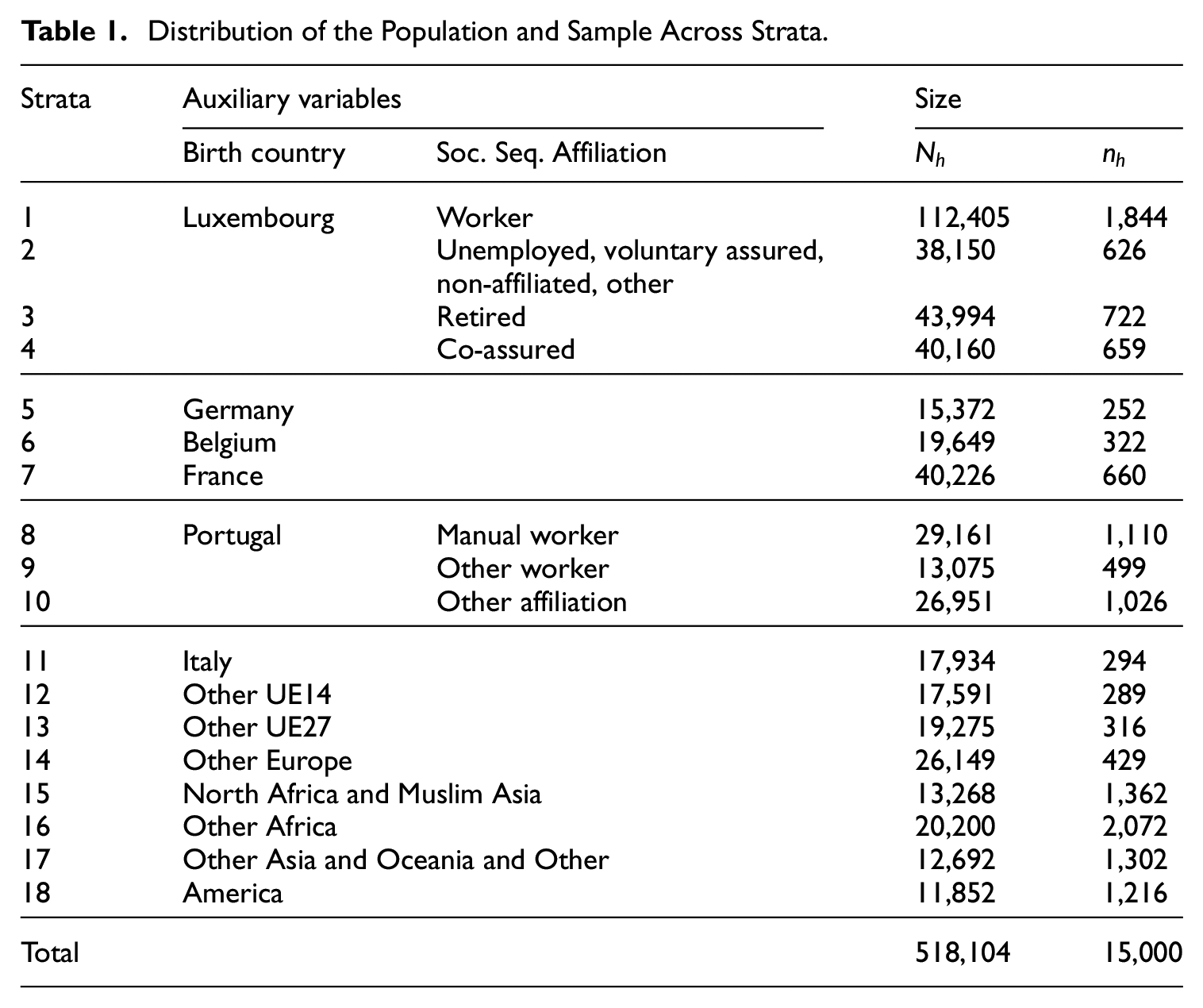
The study population is defined as the people residing in Luxembourg in October 2020, aged eighteen years and older (age defined as at December 2020). For this survey, the study population coincides with the reference population. The sampling frame of the reference population is defined with the existing administrative registers in Luxembourg, precisely the register of the physical persons (RNPP in French) and the register of affiliated individuals in the Luxembourgish social security, held by the Inspection of social security (IGSS, in French). These two registers contain the main socio-demographic information (age, gender, nationality, …) and basic socioeconomic information such as characteristics of employment (if any) and gross salary or other social benefits (see Inspection Générale de la Sécurité Sociale 2022, for further details). After some cleaning, the size of the reference population is set at 518 104 individuals.
3.2. Sampling Design
The selection of the sample is done facing two constraints: firstly, it should be possible to compute the variance of the considered estimators (mainly totals and means, but also ratios); secondly, the study requires an efficient analysis of the opinions for the minority groups. It is well know that those groups are reluctant to reply. There should therefore be, at least at the sampling phase, a minimum number of individuals sampled within this category. A stratified without-replacement probabilistic sampling design is chosen. The stratification variable is a combination of groups of birth countries, and for some of those groups the affiliation status to the social security. Precisely, birth countries are divided into thirteen groups: Luxembourg; Germany; Belgium; France; Portugal; Italy; Other European Union (EU) 14; Other EU27; Other Europe; North Africa and Muslim Asia; Sub-Saharan Africa; Other Asia (including Oceania and others); America. The birth country Luxembourg is divided into four groups, depending on the status of social security affiliation (workers-of any type; unemployed and non affiliated to the social security; retired; coinsured—insured by means of another person). The sub-population of citizens living in Luxembourg and born in Portugal has experienced a continuous growth since the implementation of guest-workers programs for manual (low-educated) workers in 1970 (Heinz et al. 2013) and then the economic crisis (Hartmann-Hirsch and Amétépé 2023). Portuguese citizens represented 16% of Luxembourg’s population in 2011, and 14.5% in 2021 (Klein and Peltier 2023). They also represent the largest foreign community among the immigrant population, with 30.8% in 2021 (Klein and Peltier 2023). For web-mode surveys, it is well know that low educated individuals tend to have a lower response rate. Moreover, previous experience with surveys indicate that Portuguese are not receptive with the web mode either (Mathä et al. 2023). Benefiting from the large number of people born in Portugal, we can partition this strata into three groups using the working status as a proxy of education. Then, the birth country Portugal is split into three groups of social security affiliation (manual workers; other type of workers; other type of affiliation). Overall, there are
A sample allocation of 15000 individuals is done under the following criteria. Firstly, proportional allocation across strata of 8500 individuals. Secondly, allocation of 1500 individuals in the strata of people born in Portugal. Thirdly, an allocation of 5000 individuals into the strata of people born outside European countries. The over-sampling inside those strata corresponds to an anticipated lower response rate, which has been observed in previous surveys. Therefore, a minimum sample size (achieved with the over-sampling) is settled to try to reach a sufficient number of respondents to have efficient estimations. Table 1 displays the totals population/sample size by stratum.
Distribution of the Population and Sample Across Strata.
3.3. Non-Response Correction
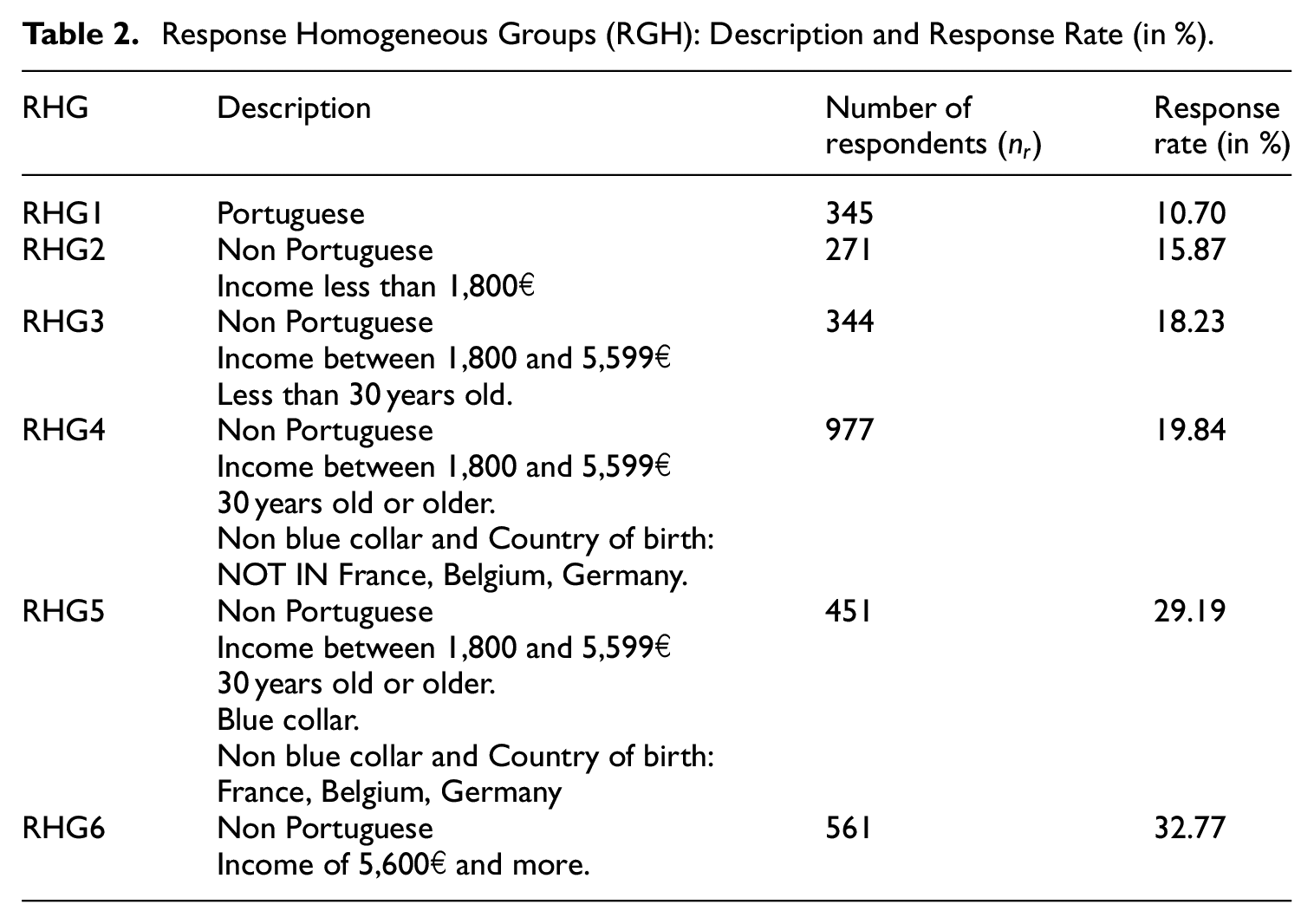
After one month of fieldwork, there are 2949 valid responses (around 20% response rate). Since we are no longer working with the probability sample but only with a sub-sample, we might introduce non-response bias. Indeed, the behavior of the respondents may differ from the behavior of the non-respondents. To correct for the non-response, the well-know method of Response Homogeneity Groups (RHGs) is implemented (Särndal and Swensson 1987). This method consists in partitioning the sample so that the response in each group is quite homogeneous, but different from the other groups. In practice, five auxiliary variables explain the non-response: nationality, income class, age class, affiliation status to the social security, and country of birth. The RHGs are defined in Table 2, where the number of respondents and the response rate are also given for each group. We wish to highlight the variability in the response rates. On the one hand, the response rate of Portuguese citizens/nationals is very low, and approximately half of the average response rate. On the other hand, the non-Portuguese with income greater than 5600€ have the highest response rate, which is about 33%. These differences state clearly that there could be some non-negligible bias introduced by non-response if no correction is applied.
Response Homogeneous Groups (RGH): Description and Response Rate (in %).
3.4. Calibration on Margins
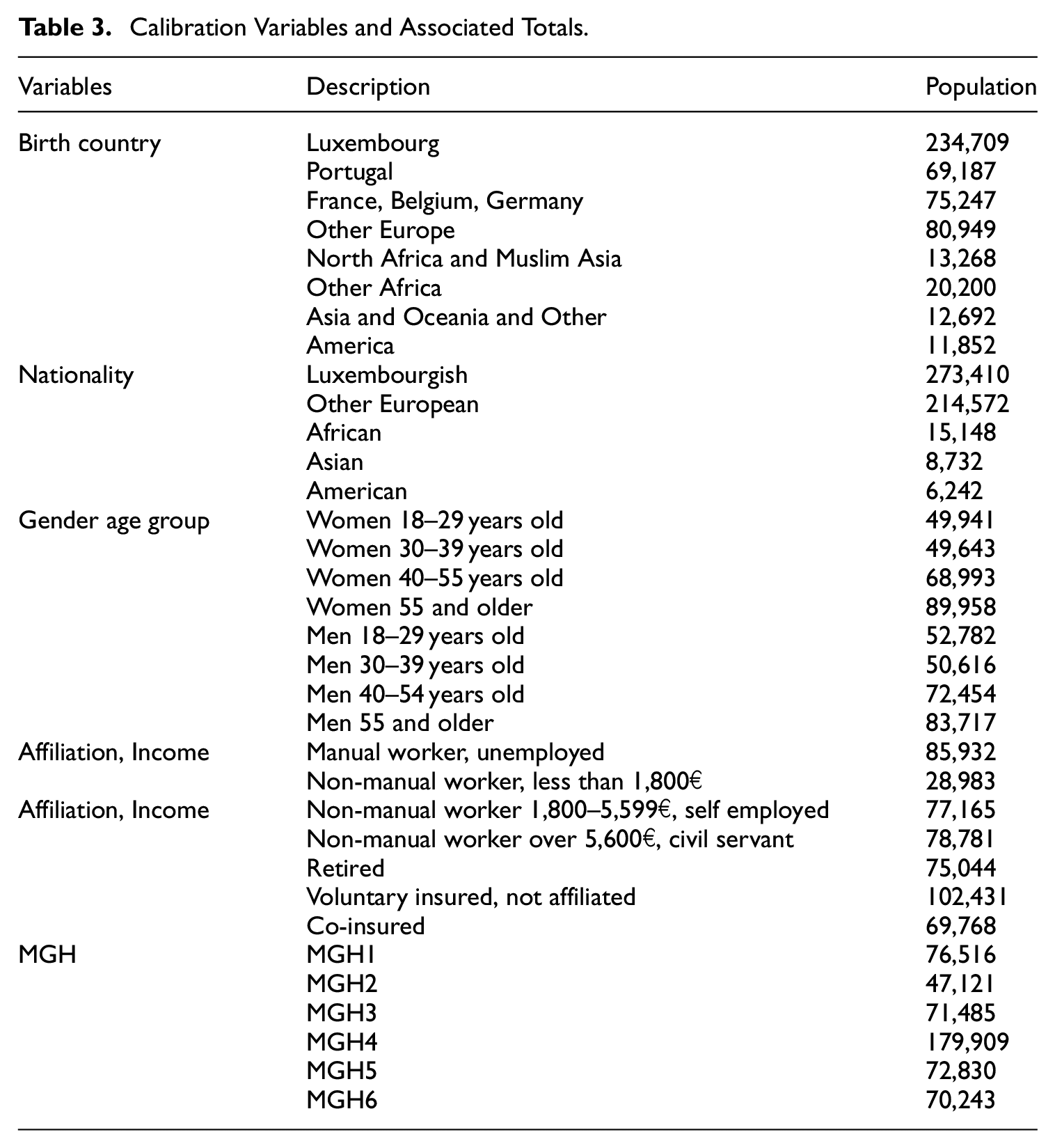
The last step is the so called calibration on margins. The idea is to adjust the data from the survey to external population totals. Usually, this calibration is done after the non-response correction. Apart from the RHG defined before (see Table 2), the calibration variables are: Country of birth (Luxembourg; Portugal; France, Belgium, Germany; Other Europe; North Africa and Muslim Asia; Other Africa; Asia, Oceania and Other; America); Nationality (Luxembourgish; Other European; African; Asian; American); gender and age group (women: 18–29 years old; 30–39 years old; 40–45 years old; 55 and older; men: 18–29 years old; 30–39 years old; 40–45 years old; 55 and older); combination of affiliation status and income class (manual worker and unemployed; non-manual worker with income lower than 1,800€; non-manual worker with income 1,800 to 5,999€ and self-employed; white collar with income higher than 5,600€ and civil servant; retired, invalid or pre-retired; voluntary assured and non-affiliated); co-insured. The auxiliary variables used for the calibration are given in Table 3. The calibration was performed with the raking ratio distance function (Deville and Särndal 1992). The CALMAR macro (Sautory 1993) allows east implementation of the calibration procedure with the SAS software.
Calibration Variables and Associated Totals.
4. Application
In this section, we compare the results obtained with the analytic variance estimator presented in Subsection 2.1, and the bootstrap variance estimator presented in Algorithm 3, when estimating a proportion. From the data described in Section 3, we consider the following variable of the questionnaire (Docquier et al. 2022): Regarding your attitude toward racism (hierarchies between human groups related to skin color, country of origin, religion, the consonance of a surname/given name, clothing and cultural practices, etc.), which of the following statements comes closest to your view?
(1) Human races do not exist.
(2) All human races are equal.
(3) There are races superior or inferior to others.
(4) No response.
(5) I don’t know.
Our aim is to estimate the distribution of the responses for the question, which can be also calculated as the proportion of people replying yes to each statement. The modalities are exclusive, and we can therefore transform it into 5 dummy variables.
We define the variable of interest
for
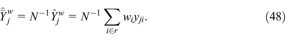
The analytic variance estimator
The results for each question
Estimated Proportion
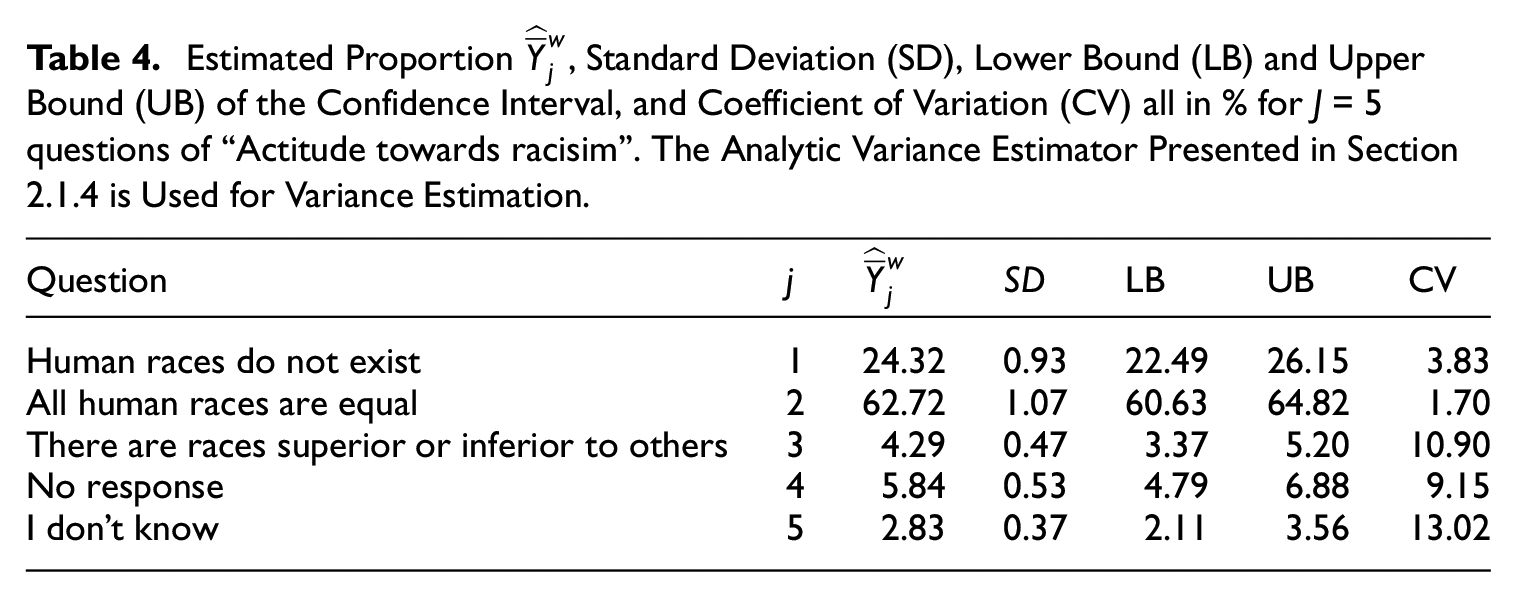
The coefficient of variation is relatively low for j = {1, 2}, since more than half of the respondents chooses this modality. However, for j = 3 the CV is higher than 10%. We highlight the statements j = {2, 3} since those are the statements where there are more respondents (j = 2) or where the respondents are more scarce (j = 3), respectively. We do not consider further
We then perform the bootstrap procedure presented in algorithm 3, using the raking ratio distance function in Step 4. We obtain four vectors of
We compute a normality-based confidence interval (CI) using the analytic variance estimator in Equation (22)

where
Secondly, the percentile confidence interval relies upon the assumption that the conditional distribution of the bootstrap calibrated estimators in Equation (39) is a good approximation of the distribution of the calibrated estimator
Thirdly, the reverse percentile confidence interval (a.k.a. basic confidence interval) uses of the conditional distribution of

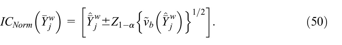
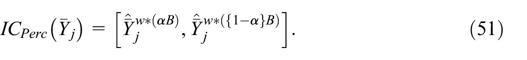
We first study the distribution of the bootstrap calibrated estimators
Empirical and theoretical density (top left), Q-Q plot (top right), empirical and theoretical CDF (bottom left), and P-P plot (bottom right) for the distribution of
Empirical and theoretical density (top left), Q-Q plot (top right), empirical and theoretical CDF (bottom left), and P-P plot (bottom right) for the distribution of
Figure 3 displays the normality based confidence interval for
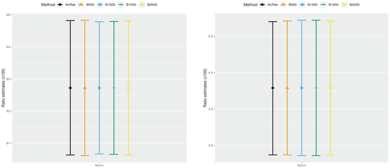
Normality based confidence intervals (Norm) for
Figure 4 depicts normality based (Norm), percentile (Perc), and reverse (PercInv) confidence intervals for
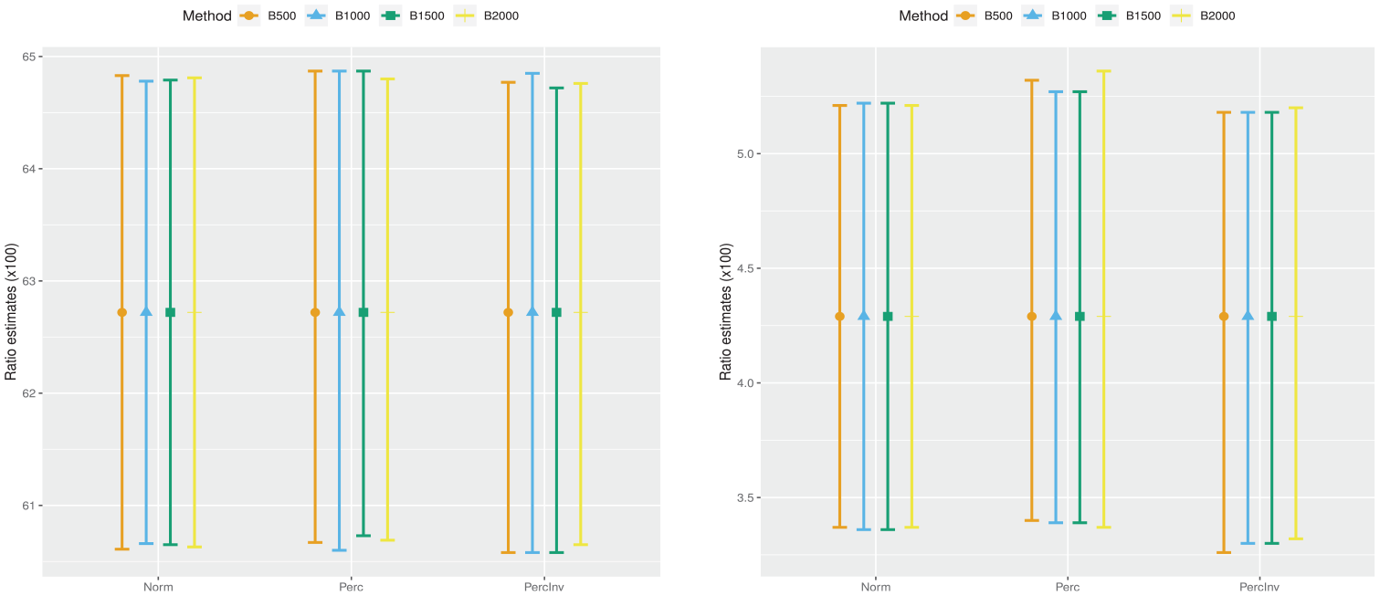
Normality based (Norm), percentile (Perc), and reverse (PercInv) confidence intervals for
4.1. Simulation Study
We perform a simulation study to evaluate the performance of analytic and bootstrap variance estimators. We consider a realistic population, based on the survey “Racism and discrimination ethno-racial.” From the subset of respondents, we create a pseudo-population by duplicating each observation, using the calibrated weight rounded to the closest integer for the number of duplications. This leads to a pseudo-population of 518 094 individuals.
We consider two variables from the questionnaire. Firstly, the same variable as in Section 3, only for the cases
The sampling design and the non-response pattern are the same as in the real survey. A stratified simple random sample
For a binary variable
where
where
For example, for the estimation of the proportion for people with a low education level, we have
The linearized variance estimator
For all the estimators in Equations (53) to (56), we also compute a bootstrap variance estimator obtained by applying Algorithm 3 with

with
where
Also, we compute the coverage rates of the confidence interval associated to the percentile bootstrap, to the basic bootstrap and to the normality-based confidence interval, with nominal one-tailed error rate of 2.5% in each tail.
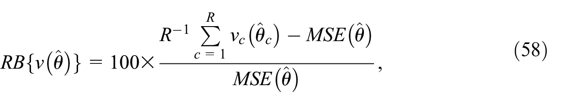
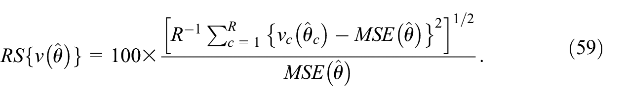
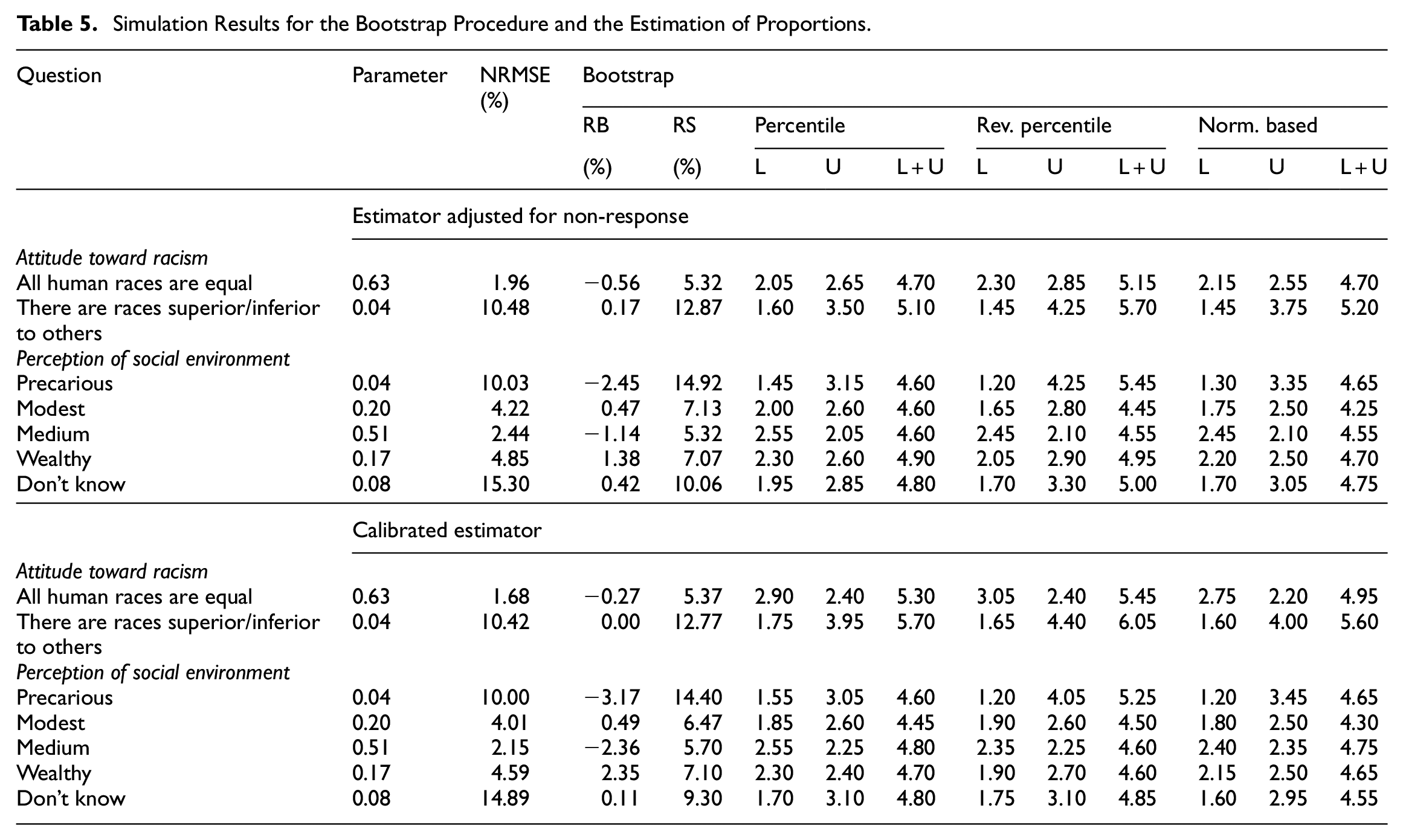
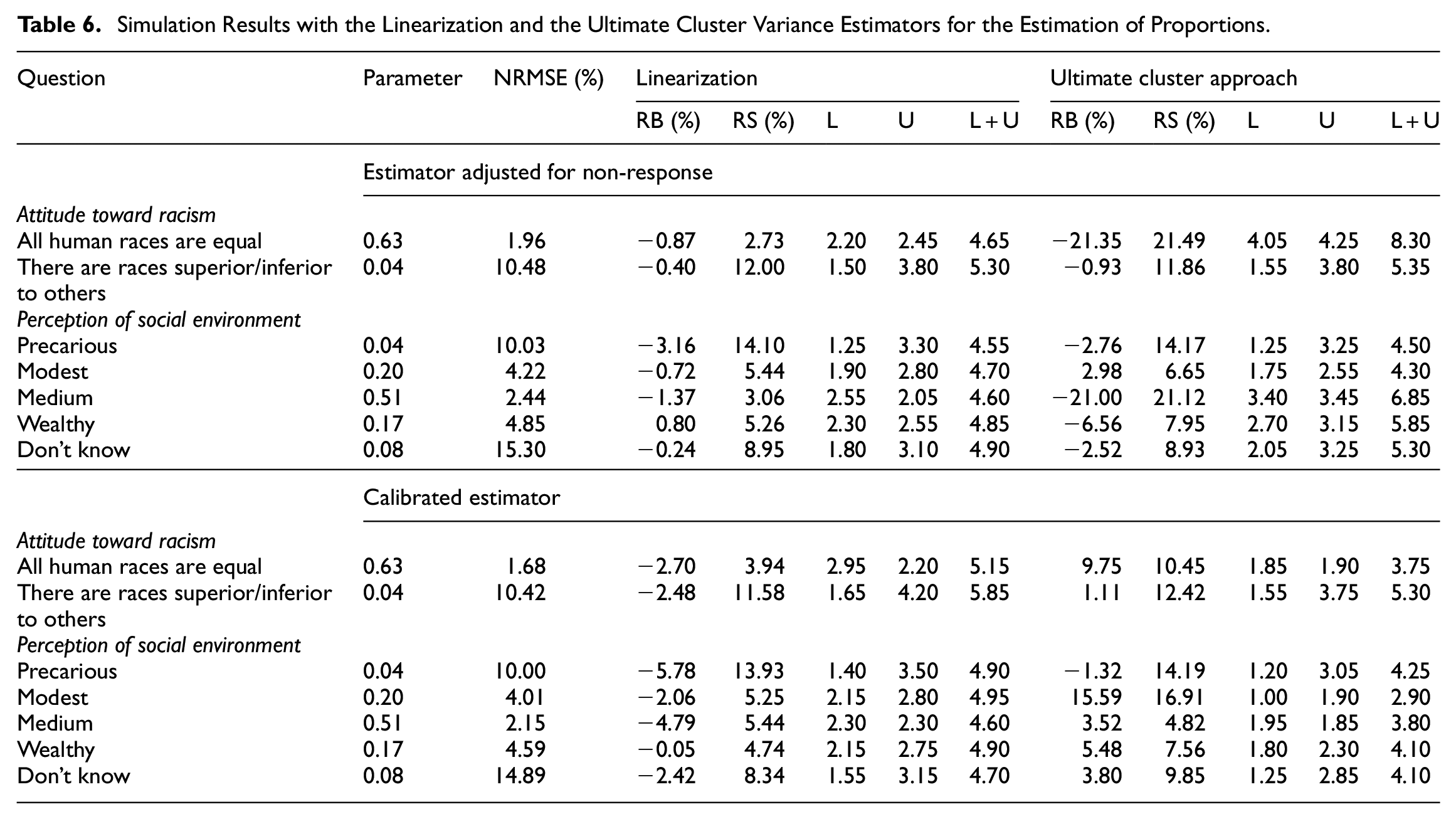
The simulation results for the estimation of proportions are given in Table 5 for the bootstrap, and in Table 6 for the linearization and the ultimate cluster approach. We first note that the NRMSE is smaller with the calibration, as could be expected, although the gain in efficiency is moderate. The bootstrap variance estimator is almost unbiased in all cases, with RB no larger than 4%. We note that the fact that we did not include the finite population corrections inside strata does not affect the performance of the bootstrap variance estimator. The linearization variance estimator tends to be slightly negatively biased, but the absolute RB is no larger than 6%. In terms of RS, the linearization variance estimator is usually slightly more stable. The coverage rates are fairly well respected in all cases for the three bootstrap procedures for interval estimation, and for the normality-based confidence interval with the linearized variance estimator. As expected (see Subsection 2.2.2), the ultimate cluster variance estimator is usually negatively biased for the estimator adjusted for non-response. The bias is particularly large if the proportions are close to 0.5 (in which case, the variability of the estimated proportion is larger). In case of the calibrated estimator, the ultimate cluster variance estimator is positively biased, which is due to the fact that the variance reduction due to calibration is not accounted for. The RB is as high as 16% for the calibrated estimation of the proportion of people who perceive their environment as modest. As expected, the coverage rate is too small if the ultimate cluster variance estimator is negatively biased, and too large if it is positively biased.
Simulation Results for the Bootstrap Procedure and the Estimation of Proportions.
Simulation Results with the Linearization and the Ultimate Cluster Variance Estimators for the Estimation of Proportions.
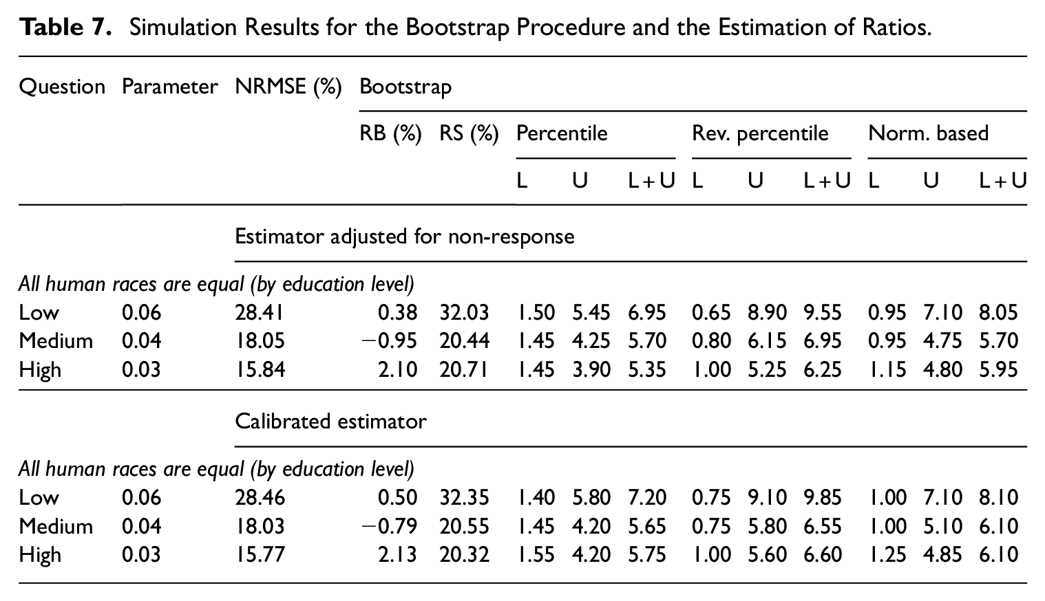
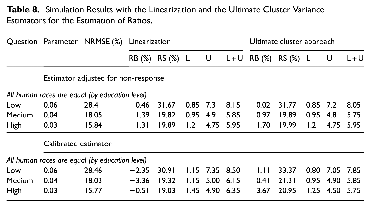
The simulation results for the estimation of ratios are given in Table 7 for the bootstrap, and in Table 8 for the linearization and the ultimate cluster approach. In terms of NRMSE, there is virtually no difference between the estimator adjusted for non-response and the calibrated estimator. All the variance estimators perform well in terms of RB, which are no larger than 4% in all cases, and perform similarly in terms of RS. Concerning the confidence intervals, we note that in all cases the coverage rates are not well respected in each tail, which is likely due to the fact that the distribution of the estimated ratio is skewed. Overall, the percentile bootstrap performs slightly better and the reverse percentile bootstrap performs slightly worse. The three normality-based confidence intervals perform similarly.
Simulation Results for the Bootstrap Procedure and the Estimation of Ratios.
Simulation Results with the Linearization and the Ultimate Cluster Variance Estimators for the Estimation of Ratios.
5. Conclusions
In this article, we have compared the rescaled bootstrap with the linearization and the ultimate cluster variance estimator. Our simulation results indicate that the bootstrap and the linearization perform similarly in terms of relative bias of the variance estimator. On the other hand, the ultimate cluster variance estimator can be strongly biased for estimating the variance of the estimator of the total. The good performance of the bootstrap was not necessarily expected, since the sampling fractions in some strata are not negligible. Bootstrap seems therefore a viable approach, even with moderate sampling fractions.
These results may be interesting to the survey data users, who rarely have access to all the information needed to compute the analytical variance; namely, the design variables, and the auxiliary variables used for the definition of the response homogeneity groups or for calibration.
For non-linear parameters, the variance may be estimated by using the linearization technique, which is somewhat laborious since a specific linearized variable needs to be computed for each parameter. On the other hand, the bootstrap makes it possible to estimate the variance by simply computing the dispersion of the bootstrapped versions of the estimator. The approach is therefore straightforward for data users, once replicated weights accounting for all the estimation steps (non-response and calibration) are released with the survey dataset.
The sampling design used in the survey on racism is relatively simple, since a sampling frame is available in the target population. Unfortunately, this sampling design is not very common for household and social surveys, for which some form of multistage sampling is more likely. An evaluation of the rescaled bootstrap on a real-life multistage survey would be of great practical interest. In other cases, a sampling frame is not available, and the target population may only be surveyed through an intermediary population by means of indirect sampling (Lavallée 2007), and by using the weight share method (Deville and Lavallée 2006). Variance estimation is somewhat complex in case of indirect sampling, since a synthetic variable needs to be used in the variance estimator (e.g., Chauvet et al. 2023). A valid bootstrap procedure for indirect sampling would be both of theoretical and practical interest.
Like many sample surveys, the survey on racism and discrimination suffers from significant non-response. In this context, it is particularly important to model the non-response mechanism as well as possible, in order to obtain adjusted estimators making it possible to limit the bias due to non-response. Beyond its use for variance estimation, bootstrap can also be used to compare the effectiveness of estimators adjusted for non-response, for example by testing the division of the sample into finer homogeneous response groups. This is an aspect that would be very important for users, which we plan to invest in.