
Abstract
If part of a population is hidden but two or more samples are available that each cover parts of this population, multiple systems estimation can be applied to estimate the size of this population. A problem is that these estimates suffer from finite-sample bias that can be substantial in case of a small sample or a small population size. This problem was recognized by Chapman, who derived his essentially unbiased Chapman-estimator for two samples. Because more than two samples may be required to correct for sample dependence, we propose a Generalized Chapman-estimator that can be applied with any number of samples. In a Monte Carlo experiment, this new estimator shows hardly any bias and has smaller standard errors than competing bias-reduced estimators. It is also compared to the usual maximum likelihood estimates for the case of estimating the number of homeless people in the Netherlands, where it shows notably different outcomes.
1. Introduction
Estimating the size of a closed population, which is partly observed through a set of incomplete samples that each cover parts of this population, is an important statistical problem. The estimation method for this problem is known as multiple systems estimation (MSE), but also as capture-recapture, mark-recapture, or multiple-recapture estimation. An overview of its history and applications is provided by for example, Bird and King (2018), Cormack (1989), and International Working Group for Disease Monitoring and Forecasting (1995). The most basic MSE estimator was proposed by Petersen (1896) and later Lincoln (1930) and is therefore known as the Lincoln-Petersen (LP) estimator. The LP-estimator is based on two random population samples, and under a set of assumptions discussed in Wolter (1986), it provides an asymptotically unbiased estimator for the size of the population.
Two of the main assumptions are the assumption of sample independence and of homogeneous inclusion probabilities of population units. A standard approach that aims to correct for this bias is the incorporation of additional samples and covariates in the MSE model (see, e.g., Bishop et al. 1975). Fienberg (1972) showed that the log-linear model provides an easy and flexible way of incorporating multiple samples, covariates, and relations between them into MSE. The standard approach of estimating the parameters of a log-linear model, is by maximum likelihood (ML). A well-known problem of ML estimates of log-linear model parameters is their bias in finite samples (see e.g., Hald 1952, chap. 7, or Miller 1984), which can be substantial in case of small samples (Long 1997, 53–4; Rainey and McCaskey 2021). We should note that this “bias” refers to mean-bias and not median-bias, because median-unbiasedness is not affected by non-linear transformations (see, e.g., Hald 1952; Kosmidis et al. 2020, for further discussion). In fact, the reduction of mean-bias often leads to the introduction of median-bias, so there is a trade-off involved. However, as discussed by for example, Kosmidis and Firth (2021) and Rainey and McCaskey (2021), another advantage of mean-bias reduction, is that it also reduces the variance and therefore the accuracy of the ML-estimator and so it is generally desirable.
For the LP-estimator bias was already discussed by Chapman (1951) and Bailey (1951), who each propose their own alternative estimator with improved finite-sample properties. Chapman (1951, 147) showed that his estimator is “essentially unbiased” and so his Chapman-estimator became the standard bias-corrected version of the LP-estimator. A problem with both the Chapman- and Bailey-estimator is that they are designed only for two samples, so it is unclear how they can be applied in case there are more than two samples. This is important, because to paraphrase Tilling (2001), bias in MSE estimates is more likely if one sample (or a combination of samples and/or categorical covariates) contains very few records, which becomes more likely in case more samples (or covariates) are involved. Chapman (1952) himself extended his estimator to more than two samples, but only for the case where a unit was tagged in an earlier sample or not, and therefore it cannot be used with a log-linear model that contains sample dependencies, which requires the availability of complete inclusion patterns. Evans and Bonett (1994) and Rivest and Lévesque (2001) propose bias reduction methods specifically for MSE that are, as in Firth (1993), Kosmidis and Firth (2011), and Kosmidis et al. (2020), based on modified score-functions. They propose modification schemes for the log-linear models by Otis et al. (1978), which correspond to a selection of log-linear model specifications (Chao 2001).
In this article, we derive a generalization of the Chapman-estimator, which can be applied with any log-linear model specification. For two samples our Generalized Chapman-estimator is, just like the estimator by Rivest and Lévesque (2001), equivalent to the Chapman-estimator and for more than two samples it differs from the estimator that is proposed by Rivest and Lévesque. To derive this new estimator, the next section introduces some notation and discusses the relation between MSE and the log-linear model, the problem of bias, and bias correction.
2. Multiple Systems Estimation Theory
MSE considers a closed population of size
2.1. The Saturated Log-Linear Model
Fienberg (1972) showed that MSE can be described by a log-linear model, that for two samples is written as

where

Asymptotic consistency of the LP-estimator relies on the assumption of independence between sample

In this case of three samples, for identification it is generally assumed that the three-way interaction parameter

and for
where
2.2. The Chapman-Estimator and a Generalization for Saturated Models
The conditional ML-estimators discussed in the previous section suffer from finite-sample bias (see e.g., Hald 1952, chap. 7, or Miller 1984). A straightforward example is provided by the LP-estimator in Equation (2), which has no finite expectation because there is a non-zero probability of

Chapman (1951, 146) shows that if the two samples are large enough compared to
which converges to zero for large enough
A reason why Chapman’s derivation is powerful is because Chapman uses the inverse factorial approximation, which for the function
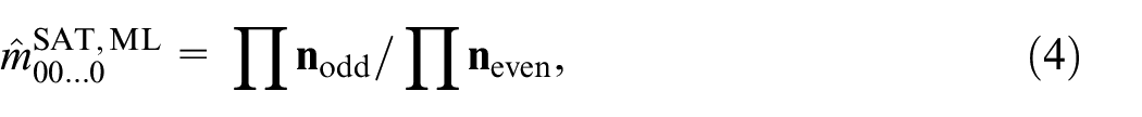
The Chapman-estimator can be derived by assuming that the set

Under Poisson sampling, combining Equation (7) with Equation (4) gives a new bias-corrected estimator for

For the saturated model with three samples as defined in Equation (3), Equation (8) gives

This estimator can also be obtained with the modified-score function approach, by replacing

The idea of adding 1 to each variable in the denominator was also suggested in a slightly different context by Jewell (1986), who was interested in an estimate of the odds ratio of a
The Generalized Chapman-estimator in Equation (8) is a bias-corrected estimator for saturated models. The next section shows that if an unsaturated model is chosen, this leads to a different optimal modification scheme and therefore a different bias-corrected estimator.
2.3. Unsaturated Log-Linear Model Specifications
A log-linear model (LLM) for any number of samples and parameters can be written as

with
Fienberg (1972) discusses three typical unsaturated models for the case of three samples, which are illustrative for our purpose. We refer to them as the two-pair dependence (2PD), the one-pair dependence (1PD), and independence (IND) model, which are


The 2PD and 1PD model may also be formulated with different pairwise interaction terms, but because we can change the order of samples without loss of generality, we can limit ourselves to these three models. For the 2PD and 1PD model, Fienberg (1972, 596) derives closed form expressions of the conditional ML-estimators for


Fienberg (1972) further shows that for the independence model a closed form expression of
The optimal modification schemes for the estimators in Equations (14) and (15) can be easily derived when Equation (7) is considered.


as bias-corrected estimators for the 2PD and 1PD model. This shows that in case of the 2PD model the optimal modification scheme for the saturated model is overdone but not incorrect, because

as a bias-corrected estimator, which differs from the optimal
The derivation of the bias-corrected estimators in Equations (8), (16), and (17) requires closed form expressions of the ML-estimators for
2.4. The Generalized Chapman-Estimator
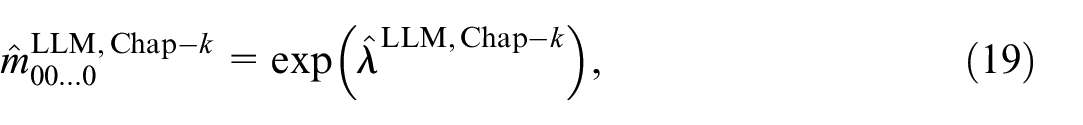
The previous section showed how a closed form expression of the ML-estimator for
where
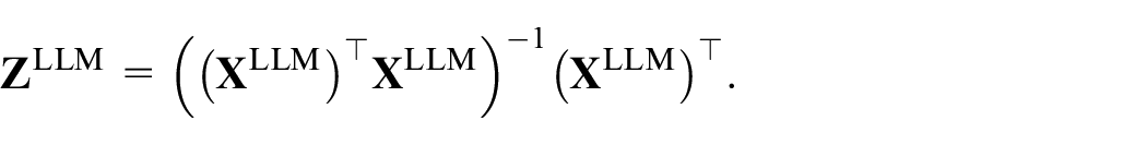
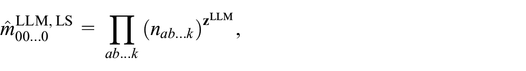
Because the rank of
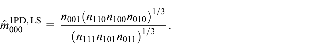
This LS-estimator resembles the ML-estimator for the 1PD model as given in Equation (15), in the sense that they are both fractions of means over the same elements of
The relation between the LS- and ML-estimator for the SAT, 2PD, and 1PD model can, by using
The Value of
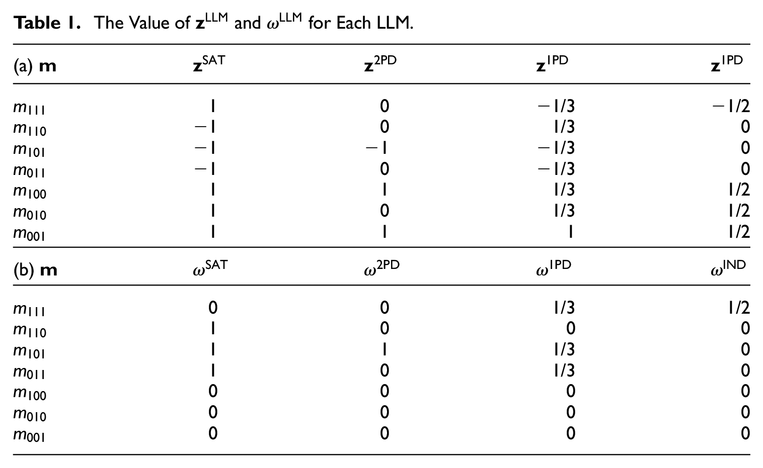

where
with
Finally, in this section the design matrix
2.5. Other Bias-Reduced MSE Estimators
Evans and Bonett (1994) and Rivest and Lévesque (2001) propose bias reduced MSE-estimators for log-linear models with more than two samples. They are, just like
Rivest and Lévesque (2001) propose a more sophisticated MSE modification scheme that is, for the two sample model in Equation (1), equivalent to the Chapman-estimator. In a Monte Carlo simulation study they show that their RL-estimator has less bias than the EB-estimator for all the models by Otis et al. (1978). For more than two samples, the modification scheme by Rivest and Lévesque (2001) differs from the modification scheme proposed in Equation (18). This is clearly shown by the difference in

and (see Rivest and Lévesque 2001, 562)

Rivest and Lévesque also develop a modification scheme for the so-called

For other unsaturated models, such as the 2PD and 1PD model, Rivest and Lévesque do not specify a specific modification scheme, therefore in the simulation studies in the next section, in such cases we use the modification scheme for model
3. Simulation Studies
In this section the generalized Chapman-estimator is compared in three Monte Carlo simulation studies, that each considers a set of different scenarios. The scenarios differ from each other by
The first simulation study is straightforward and only considers two samples and seven scenarios. The second and third simulation study both consider three and four samples in fifteen scenarios. The difference between the second and the third simulation study is the log-linear model that is used for estimation. In the second study the population size estimates are obtained from an assumed saturated log-linear model as in Equation (3), and in the third study the population size estimates are obtained under the assumption of the correct log-linear model specification (see Table 4). The use of the correct model specification may not be realistic in practical applications, but the results of this study show how the Generalized Chapman-estimator performs in case of other unsaturated models.
We should note that when a model contains redundant parameters as occurs with the saturated model in the second study, the resulting estimates have a larger variance (Bishop et al. 1975, 242). This additional variance does in itself not lead to biased estimates, but it does inflate bias. This inflationary effect can be seen when the bias is written as
Another minor but important simulation issue is what Otis et al. (1978, 125) refer to as “failures.” A simple example of a failure is the LP-estimator with
3.1. Simulation Study with Two Samples
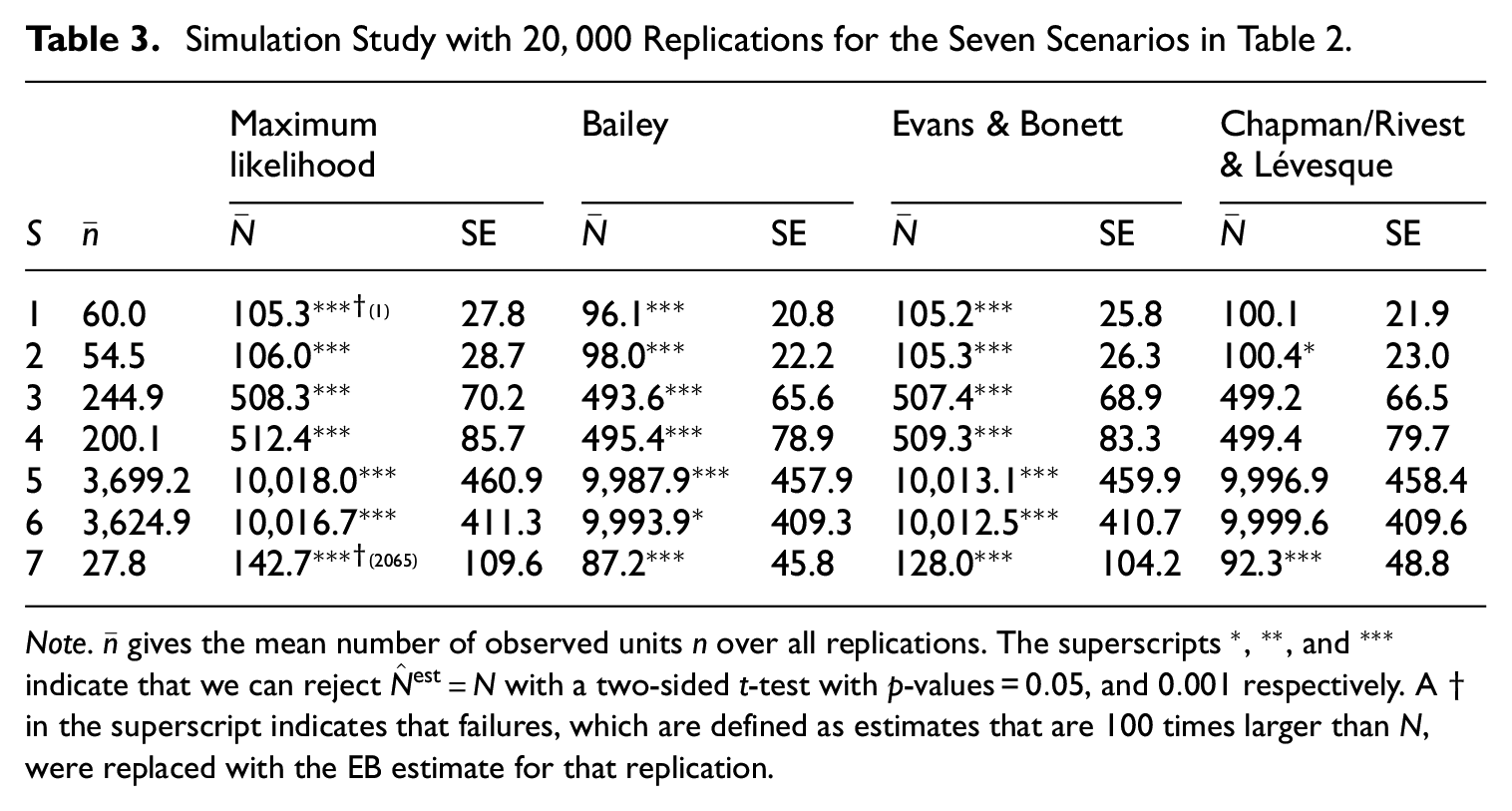
This section presents the results of a simulation study that compares the LP, Bailey, EB, RL, and Chapman estimator in case of two samples. The simulation settings for
Seven Scenarios for a Two Sample Simulation Study.
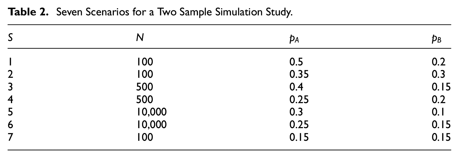
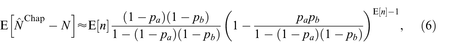
According to the expected bias expression in Equation (6), the bias in the Chapman-estimator should be small in scenario
Table 3 shows the results for the mean estimates
Simulation Study with
Note.
3.2. Simulation Studies with Three and Four Samples
This section studies which estimator should be preferred in case of three or four samples, for which the RL-estimator and Generalized Chapman-estimator are no longer equivalent as in the previous section. This section contains two simulation studies. The first simulation study uses the saturated log-linear model for estimation and the second simulation study uses the correct unsaturated log-linear model for estimation. Each simulation study considers the same fifteen scenarios, indicated by
Three and Four Sample Simulation Scenarios.
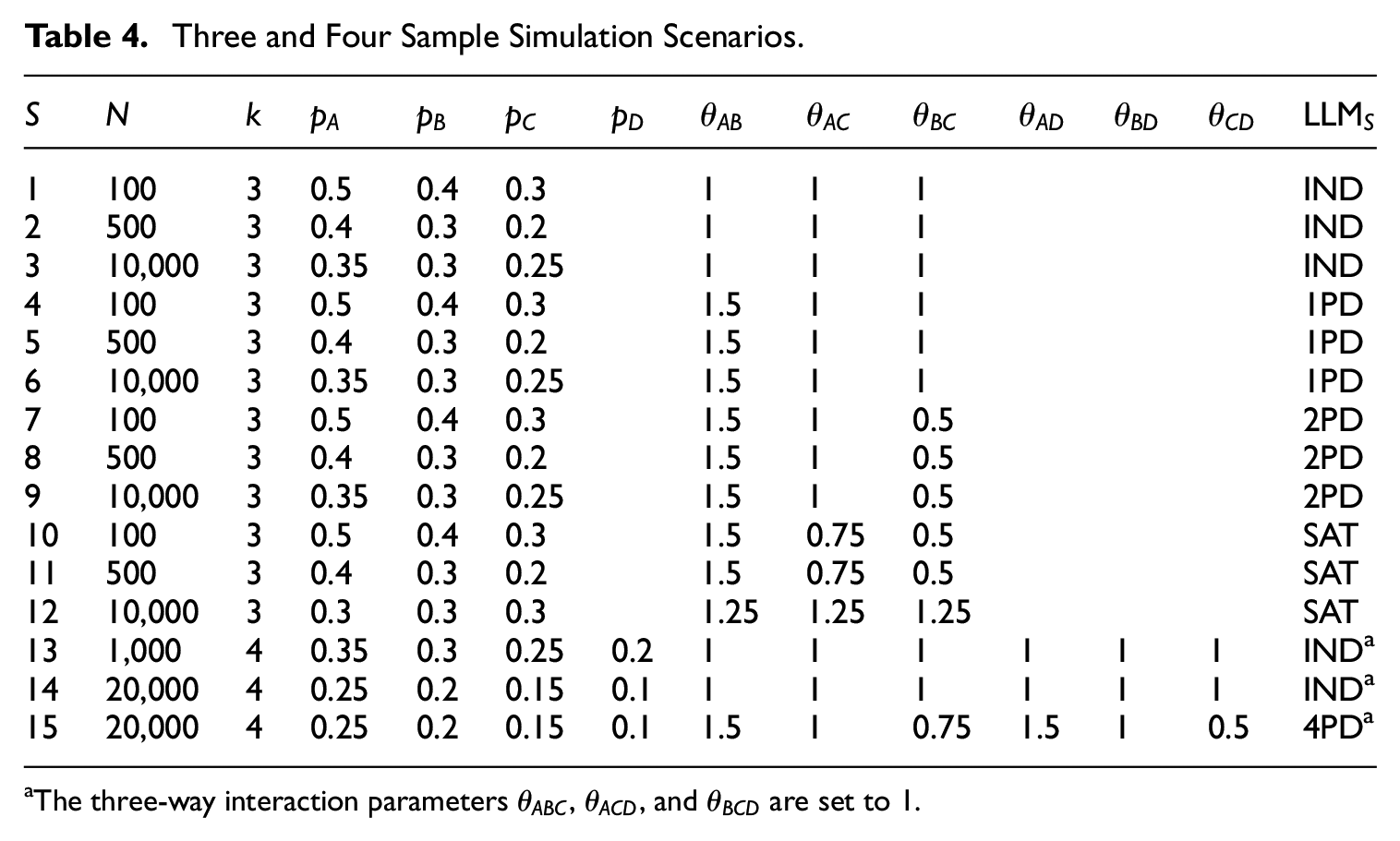
The three-way interaction parameters
3.2.1. Results for the Saturated Log-Linear Model
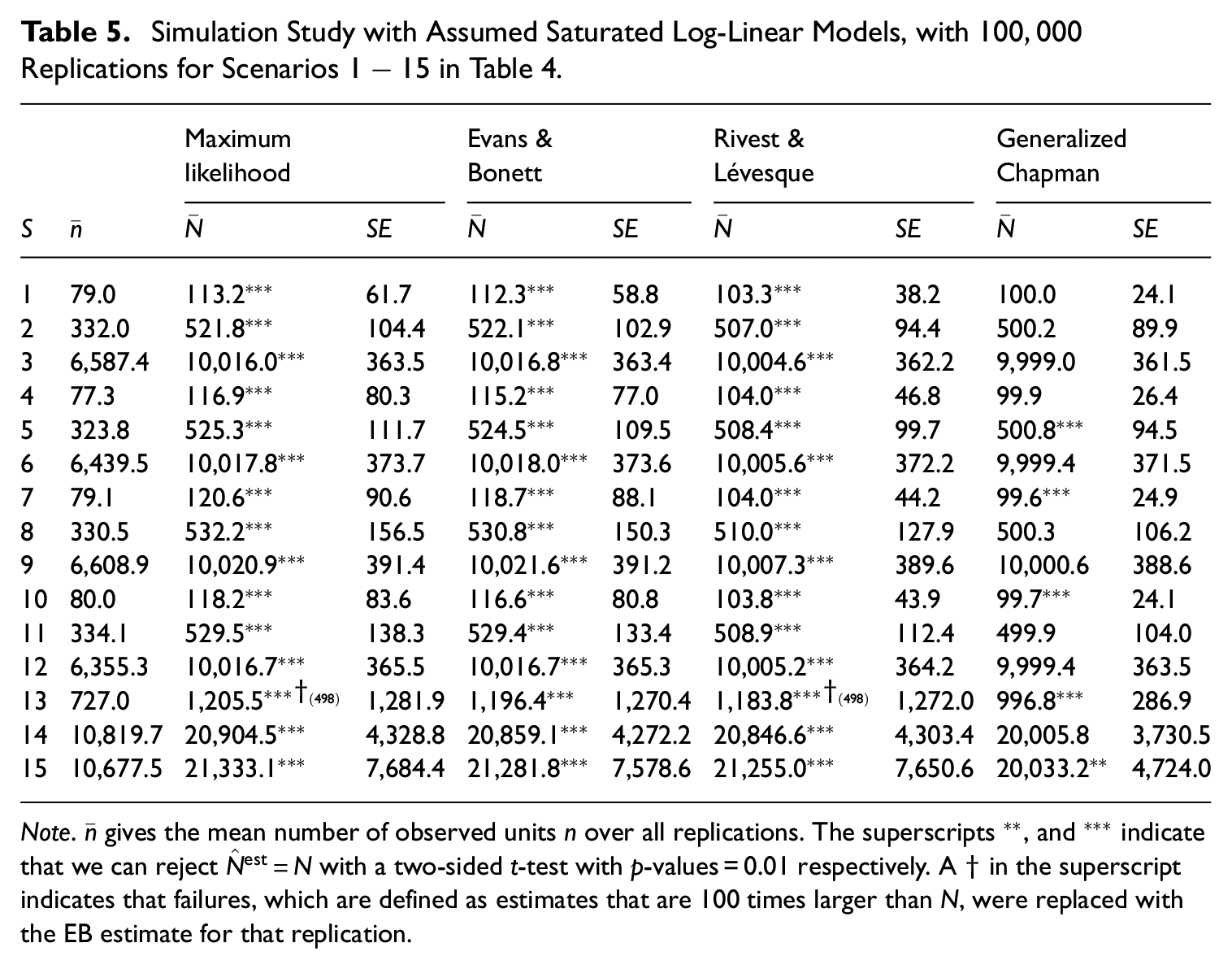
The results presented in Table 5 show that, for an assumed saturated model, the Generalized Chapman-estimator performs best of the tested estimators in each scenario. For
Simulation Study with Assumed Saturated Log-Linear Models, with
Note.
The Generalized Chapman-estimator not only outperforms the other estimators in terms of smaller mean bias, also the SEs are substantially smaller. This holds especially for scenarios with smaller
3.2.2. Results for Unsaturated Log-Linear Models
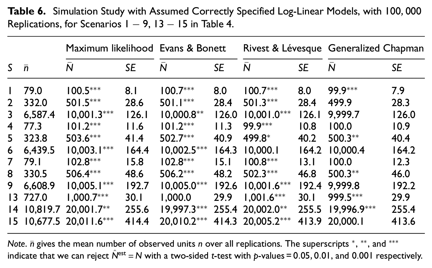
Table 6 shows the result of a simulation study that uses the same scenarios as in Table 4, but now the estimates are based on the correct unsaturated log-linear models. The results of the scenarios
Simulation Study with Assumed Correctly Specified Log-Linear Models, with
Note.
Modification schemes for unsaturated models with four samples, as in the last three scenarios, were not presented in Table 1 or Subsection 2.5, so for the IND and 4PD model they are given here. For the Generalized Chapman estimator and the IND model,
The results in Table 6 are, for all estimators, clearly better than those in Table 5. The use of the correct unsaturated model for each scenario has substantially reduced the bias and SEs of all estimators. However, these improvements did not affect the (in)significance of the bias. This is shown by the many *s that are still present in all columns except for the column of the Generalized Chapman-estimator, which contains relatively few. Also, although the SEs of each estimator became much smaller and more alike, the SEs of the Generalized Chapman-estimator are still the smallest. Furthermore, in scenarios where the Generalized Chapman-estimator shows some statistically significant bias, it is in most cases smaller than the bias of other estimators, which to some extend also holds for the RL-estimator. This shows that, also for unsaturated models, the Generalized Chapman-estimator performs better than the other estimators.
Particularly interesting is the performance and comparison of the Generalized Chapman-estimator with the RL-estimator in the scenarios
A comparison of the SEs in Tables 5 and 6 shows that the Generalized Chapman-estimator suffers less from overspecification, as is the case with the saturated model for most scenarios. For example, scenario
4. Example: Number of Homeless People in the Netherlands
A population size estimate of the homeless people in the Netherlands is published annually by Statistics Netherlands. This estimate is an ML estimate that is based on a MSE model that is discussed in detail in Coumans et al. (2017). The estimate is based on a log-linear model that contains three sources and several (categorical) covariates, such as gender (
In this practical example, for the years 2009 to 2018, 2020, and 2021, we replicate the model selection and estimation procedure as explained in Coumans et al. (2017). Data for 2019 are unavailable. The model selection mechanism is performed independently for each year, and so it may select a different log-linear model for each year, with different sample and covariate dependencies. However, this model selection mechanism is based on the unmodified
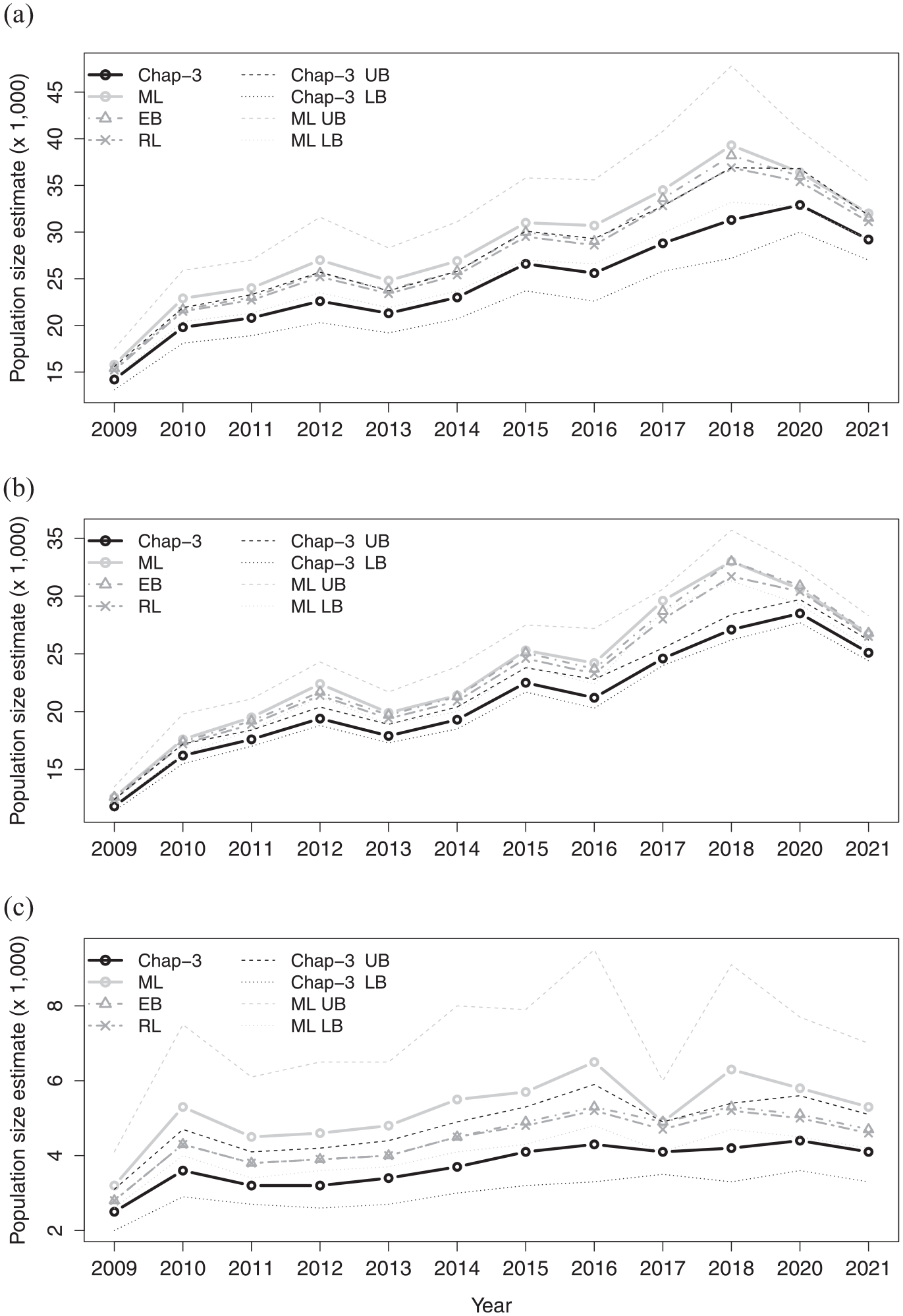
(a) Total number of homeless people, (b) homeless men, and (c) homeless women in the Netherlands over the period 2009 to 2018 and 2020 to 2021.
In each figure the EB and RL estimates (grey dotted) are always larger than the Generalized Chapman estimates (black solid) and always smaller than the ML estimates (grey solid). The ML estimates are between a minimum of 9.5% (2021) and a maximum of 25.5% (2018) larger than the Generalized Chapman-estimator. The confidence interval of the Generalized Chapman-estimators is clearly smaller. Figure 1b and c show that the total annual difference between both estimators, as was observed in Figure 1a, is not proportionally divided over men and women. In fact, the Generalized Chapman estimates have, relatively, a much larger impact on the estimate of the number of homeless women, which is the smaller group. For women the difference between the estimates is between a minimum of 19.5% in 2017 and a maximum of 51.2% in 2018.
In this practical application the impact of using the Generalized Chapman-estimator instead of the ML-estimator is larger than the impact we have seen in the simulation studies. The reason for this difference is twofold. First, the scenarios in the simulation studies were set such that the probability of estimation failures was very small, which led to a mean coverage (i.e.,
Estimated Number of Homeless People in The Netherlands in 2021, Separated by Men and Women and
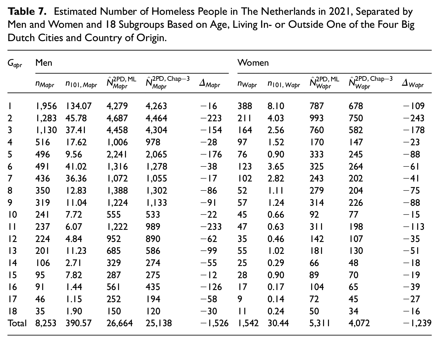
Table 7 presents
When we compare the columns
Finally, we note that the generalized Chapman estimates follow a similar trend to the ML-estimates, which is relevant from a policy perspective. From this perspective a relevant difference between the ML and generalized Chapman estimates can be observed in the years 2018 and 2020, where the ML estimate in 2020 is lower compared to 2018 while the reverse is true for the 2020 generalized Chapman estimate. This might be due to the large ML estimate in
5. Discussion
This paper presents a generalization of the Chapman-estimator and compares it to other MSE-estimators known in literature. The Generalized Chapman-estimator is first derived for saturated models and then extended such that it can deal with unsaturated models. For saturated models and a small set of unsaturated models the Generalized Chapman-estimator was derived mathematically with the help of a closed form expression of the ML-estimator. Further generalization to other unsaturated models was achieved by using the least squares estimator. The Generalized Chapman-estimator is tested in different simulation studies, which show that the Chapman-estimator outperforms other bias-reduced estimators both in terms of bias and standard error.
The derivations and simulation studies in this paper show that for any unsaturated model with three samples and some unsaturated models with four samples, or a saturated model with any number of samples, the Generalized Chapman-estimator is essentially unbiased or shows hardly any bias. We suspect that this result can be generalized toward any unsaturated model with any number of samples, although this paper does not provide a mathematical proof. We think that further research that proves, or disproves, our suspicion would be valuable.
The simulation studies also show that the bias and SE of the Generalized Chapman-estimator are less affected by overdispersion than other MSE-estimators. This advantage is important because in practice a model is usually the result of some model selection procedure, which does not guarantee the selection of the correct model and may therefore contain redundant variables.
In Section 4 the Generalized Chapman-estimator is used to estimate the number of homeless people in The Netherlands for a series of years and compares these estimates with the ML estimates. For each year both estimates are based on the same log-linear model as discussed in Coumans et al. (2017). This comparison showed that the impact of bias-correction can be substantial, for example, in our example the use of the Generalized Chapman-estimator led to an estimate that was between 9.3% and 25.4% lower for the total number of homeless people in The Netherlands, as compared to the corresponding ML-estimator. This relative difference became even larger, going up to 51%, when we zoomed in on the subgroup of women.
The simulation studies and the example in Section 4 show that the difference between the generalized Chapman- and the standard ML-estimator can be substantial. This raises the question whether finite-sample bias correction should not have a more prominent role in the discussion on the robustness of MSE methodology and the accuracy of MSE estimates, which continues till today (see e.g., Binette and Steorts 2022; Silverman 2020). Finally, in this context it would also be valuable to have expected bias expressions for MSE estimators for more than two samples, such as the bias expression by Rivest et al. (1995) in Equation (6) for the Chapman-estimator. This would give MSE practitioners more insight in the potential accuracy of their MSE estimates.
Software
All simulation studies in this paper are performed in the statistical software program R (R Core Team 2022). All estimates are obtained with the glm() function, with family = poisson(link = “log”). Differences between the LP, ML, Chapman, Bailey, EB, and RL are the sole result of different input vectors
Supplemental Material
sj-pdf-1-jof-10.1177_0282423X251314294 – Supplemental material for Bias Correction in Multiple Systems Estimation
Supplemental material, sj-pdf-1-jof-10.1177_0282423X251314294 for Bias Correction in Multiple Systems Estimation by Daan B. Zult, Peter G. M. van der Heijden and Bart F. M. Bakker in Journal of Official Statistics
Supplemental Material
sj-pdf-2-jof-10.1177_0282423X251314294 – Supplemental material for Bias Correction in Multiple Systems Estimation
Supplemental material, sj-pdf-2-jof-10.1177_0282423X251314294 for Bias Correction in Multiple Systems Estimation by Daan B. Zult, Peter G. M. van der Heijden and Bart F. M. Bakker in Journal of Official Statistics
Footnotes
Acknowledgements
The authors thank Jeroen Pannekoek, Peter-Paul de Wolf, Sander Scholtus, and Moniek Coumans from Statistics Netherlands and (anonymous) reviewers for their detailed comments and suggestions on this paper.
Funding
The author(s) received no financial support for the research, authorship, and/or publication of this article.
Supplemental Material
Supplemental material for this article is available online.
Received: January 2024
Accepted: December 2024
References
Supplementary Material
Please find the following supplemental material available below.
For Open Access articles published under a Creative Commons License, all supplemental material carries the same license as the article it is associated with.
For non-Open Access articles published, all supplemental material carries a non-exclusive license, and permission requests for re-use of supplemental material or any part of supplemental material shall be sent directly to the copyright owner as specified in the copyright notice associated with the article.