Sage Journals: Discover world-class research

Abstract

Any result from regression analysis may be subject to omitted variable bias of unknown magnitude and direction as, in practice, no dataset contains all the variables of the population model. At the same time, many variables are irrelevant and don’t contribute to the analysis. This paper explores which combination of data sources or structures will produce the best results and should be made available to the research community. We present a unified statistical framework that nests and comparable sets of constraints that characterize the effectiveness of these approaches in reducing omitted variable bias. We demonstrate our framework by estimating a wage and labor market transition model using German administrative data with a large set of linked survey variables. Overall, we find that unobserved effects panel data models with a restricted set of regressors are preferable to cross-sectional analysis with an extended set of variables. Consequently, we recommend that data providers supply administrative panel data for key variables instead of conducting extensive cross-sectional surveys.

Keywords

linked survey-administrative data endogeneity statistical regularization

1. Introduction

Official data products are increasingly based on combinations of data sources that were previously not used in official data production, such as administrative registers. New data quality frameworks are required to address various issues that are not present in survey data (Berka et al. 2012; Schnetzer et al. 2015; Zhang 2012). A body of literature already exists on the consequences of producing official statistics from linked administrative data, particularly regarding coverage and selectivity (de Wolf et al. 2019; Di Consiglio and Tuoto 2015; Harron et al. 2017; Yildiz and Smith 2015). Other literature focuses on frameworks for evaluating data quality (e.g., Oberski et al. 2017). The advantages and disadvantages of administrative data have been thoroughly elaborated by Hand (2018).

This paper contributes to the literature by considering the consequences of incomplete data structures on estimation results of regression models at the individual level. Administrative data are known to be incomplete, as they do not include all relevant variables. The omission of variables leads to biases and statistical inconsistencies in the estimated coefficients of regression models. From this perspective, we compare different cross-sectional and panel data structures commonly available to the research community. We consider both data that contain only administrative information and data that also include linked survey variables.

We present a general model compatible with a wide range of datasets and applications, though we focus on labor economics as an example. Research in economics, business, and related disciplines increasingly uses linked administrative data to benefit from larger sample sizes and higher precision in key variables, often overlooking the disadvantages of using such data, as elaborated by Hand (2018). One significant limitation is that these data only contain information generated through operational processes. Therefore, there is often a systematic lack of information on factors beyond operational processes, and even if such information is available, one should expect severe misclassification errors, requiring advanced estimation approaches (Dlugosz et al. 2017).

The existence of linked administrative data does not guarantee that all information is made accessible to researchers. In particular, not all variables are available due to data confidentiality restrictions. Tools have been developed to better understand the relevance of omitted variable bias (e.g., Gelbach 2016; Oster 2019). Rather than focusing on a single data structure, this paper builds on three common empirical strategies for reducing omitted variable bias through different combinations of data sources. While these approaches are general and not specific to one subject area, we frame the problem description and methodology illustration in the context of labor market research. The first approach is to include variables constructed from an individual’s work history as recorded in administrative data (e.g., Baptista et al. 2012; Biewen et al. 2014; Fernández-Kranz and Rodríguez-Planas 2011; Kauhanen and Napari 2012). Work history variables may directly correspond to the population model or serve as proxies for otherwise unobserved variables, such as performance. While using proxies is practically appealing, it does not guarantee bias reduction or consistent estimation. A second approach to mitigating the incompleteness of administrative variables is to incorporate survey-based variables, such as information on personality or motivation. Since the production of survey data is typically costly, it is essential to assess how much these variables contribute to the model. The third approach is to use longitudinal data, as panel models operate under weaker assumptions about the relationship between regressors and unobservables, thus facilitating analysis in the presence of omitted variables.

Despite the widespread use of work history and survey-based variables, little systematic research has been conducted to assess how effective they are in controlling for unobserved factors. Analyses aimed at investigating their role have, so far, been limited to sensitivity analyses. For example, Lechner and Wunsch (2013), Arni et al. (2014), and Caliendo et al. (2014) investigate whether the estimated treatment effects of labor market programs on labor market outcomes are sensitive to the inclusion of additional variables. Our analysis goes beyond a sensitivity analysis by suggesting statistical inference approaches to test the validity of model restrictions. We provide a formal framework for understanding estimation bias due to the omission of important variables, as well as estimation bias arising from the use of imperfect proxy variables. Our starting point is a widely used administrative data product that contains only a limited number of variables. We then assess the extent to which additional non-operational, survey-based variables and work history variables contribute to the model and alter the results. Moreover, we compare the results of cross-sectional analysis with those of panel analysis to determine how much the additional cross-sectional variables explain the variation in unobserved, individual, time-invariant effects. We apply our framework to German administrative labor market data that is linked to survey data. Based on our results, we draw conclusions about how different data structures control for unobserved factors and test the validity of the different approaches. Lastly, we derive recommendations for applied researchers and data producers.

In Section 2, the econometric problem is outlined. Section 3 describes the data, and Section 4 presents the empirical findings. The final section summarizes the results and provides recommendations.

2. The Model

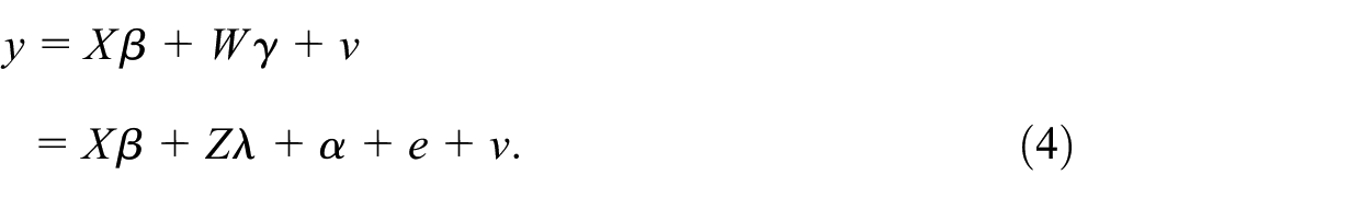
Suppose a researcher has access to some standard administrative data product with a restricted set of core variables. We consider the linear multiple regression model with population model

y = X β + W γ + v,

(1)

where β (J × 1) and γ (L × 1) are unknown parameters, X (1 ×J) are observable regressors (including the first element being a constant) and W (1 ×L) are unobserved regressors with L being unknown. We will later relax this to some of the components of W being observed. We assume that the components of X and W are not perfectly multicollinear. y is observed and v is unobserved. We assume E(v|X, W) = 0.

2.1. Omitted Variable Bias

Because W is unobserved, the model in Equation (1) cannot be directly estimated. Instead, one could omit the unobserved variables and use Ordinary Least Squares (OLS) to estimate the model

y = X β + u,

(2)

where u = Wγ+v. This is what is typically done in applications. It is well known that if there exists a j such that cov(x_j, u) ≠ 0, the OLS estimator $\hat{β}$ for β is inconsistent (e.g., Wooldridge 2010, Section 4.2.1). We focus here on a model with an unknown number of omitted variables as this is the most realistic scenario in applications. When there is more than one omitted variable, the L linear projections of W onto the observable regressors (Wooldridge 2010, 25) are

W = X 6 + R,

with δ is J × L and R is 1 ×L. Let r_l be the l’th component of R. By definition E(r_l) = 0 and cov(x_j, r_l) = 0 for j = 1, …, J and l = 1, …, L (Wooldridge 2010, 26). When plugging W into Equation (1) we obtain

y = X (β + δ γ) + R γ + v .

In this model, all regressors are uncorrelated with the composite error Rγ+v and therefore the probability limit of the OLS estimator $\hat{β}$ for model Equation (2) is

plim \hat{β} = β + δ γ .

(3)

This is the well-known omitted variables bias (e.g., Wooldridge 2010, 66–7) and its size depends on the strength of the partial correlation between W and X and the size of the elements of γ, that is, the relevance of the omitted variables in the population model Equation (1). Since W is not observed, the size and direction of the bias are unknown in an application. This is in contrast to the approach in Gelbach (2016) that focuses on variable selection. Oster (2019) thoroughly examines omitted variable bias, offering estimable expressions under constraints on unobserved variables W. The focus lies on cases where a component of X is correlated with W and requires uncorrelated components within W. We have applied her method to our problem but found the estimated proportional selection relationship to jump strongly across variables. Given this instability and that the restrictions on her model exceed what we assume in our model, we focus on alternative approaches aiming at reducing the omitted variable bias. These are presented in the remainder of this section, along with subsequent validity testing.

2.2. Proxy Variables

One approach to mitigate omitted variable bias is to plug in generated variables from the observable history of cross-section units. In labor market research these are for example variables that characterize the work history of an individual and not simply lagged observable variables. These are denoted as Z (1 ×P). It is required that none of the components of X and Z are highly correlated or perfectly multicollinear, which can be checked in an application. In most applications, P is a small integer and one should expect P ≤ L, that is, there are fewer constructed variables than omitted variables. The role of Z requires some discussion. For the reasons provided in the introduction, a special case is attained if a z_j is a proxy variable for one unobserved w_l, that is, z_j = w_l + error with E(error) = 0. However, more generally z_j can be related to any W, that is, z_j = θ₀ + Wθ_j + m_j with E(m_j|W) = 0 for all j. θ₀ (1 × 1) and θ_j (L × 1) are unknown to the researcher. If z_j is a proxy for w_l, then only the l’th element of θ_j is nonzero. This is the case that is typically considered by the proxy variable literature (Bollinger and Minier 2015; Lubotsky and Wittenberg 2006). Using Z instead of W can be also interpreted as a measurement error problem. Here any deviation from the linear combination Wθ_j, which is m_j, is the measurement error. Alternatively, one could think of z_jεW. In this case, the constructed variable would directly belong to the population model. Then m_j = 0, one component of θ_j is 1 and the others are 0. Lastly, z_j may not be correlated with any component of W. In this case θ_j = 0 and z_j should not be included at all. A researcher normally faces the problem of not knowing the exact role of the components of Z. In any case, it depends on the statistical relationship between X, W, and the m_js, whether the inclusion of Z mitigates or increases the omitted variable bias. Given that W and L are unknown, it is more convenient to write the linear projection of the linear combination of the w_ls onto the z_js, that is, Wγ = α + Zλ+e with E(e|Z) = 0 and parameters α (1 × 1) and λ (P × 1). e can be interpreted as the measurement or approximation error between Wγ and Zλ, which is the variation in the linear combination of unobserved variables that is not explained by the linear combination of constructed and included variables in Z. Therefore

\begin{matrix} y = X β + W γ + v \\ = X β + Z λ + α + e + v . \end{matrix}

(4)

For β in model Equation (4) to be consistently estimated by OLS, it is additionally required that e is uncorrelated with X and v with Z. This is not the case if X plays a role in the linear projection of Wγ on Z and X, so it is required E(Wγ|X, Z) = E(Wγ|Z). v is uncorrelated with Z is ensured by E(y|X, W, Z) = E(y|X, W), that is, the redundancy of Z in the population model. The reason for this is that in this case cov(z_j, v) = 0 for all j. Whether the bias in $\hat{β}$ in model Equation (4) is smaller or greater than in model Equation (2) is an empirical question. This depends on whether the correlations between the components of X and Wγ are greater or smaller than the correlations between the components of X and e, respectively. If for example, the size of the components of 6 are zero or very small, the inclusion of Z will increase the bias in $\hat{β}$ if there is correlation between Z and both X and v. The better the fit of the model for Wγ on Z, the more likely plugging in Z leads to bias reduction. This is because e becomes smaller in magnitude which reduces its covariance with X. It is remarked that λ has the interpretation of parameters of the linear projection on Wγ and we ignore the identifiability of α and the first component of β because the intercept is assumed to be not of interest.

2.3. Survey Data

Another approach to mitigate omitted variable bias is to enhance the regressor set by conducting a survey or by using additional administrative variables that are normally not accessible. Suppose that a subset W₁ of W, by assumption the first L1 variables of W, is observable for some random sample of the population. The idea is to do an analysis with a richer variable set. For direct comparability of the results across models, we always restrict the analysis to the cross-section units for which we have information on W₁. Thus, we ignore the potential loss in precision and focus on asymptotic bias only. We consider the case, where the researcher is primarily interested in estimating the partial relationship between y and elements of X, rather than between y and elements W₁, although the latter will be typically also of interest. W₂ is 1 ×L2 and comprises of the last L2 elements of W with L1 + L2 = L. W₂, the remaining unobservable variables, may be correlated with X and W₁. Therefore, their omission induces a bias for estimated β and γ₍₁₎ in the regression of y on X and W₁:

y = X β + W_{1} γ_{(1)} + u_{2},

(5)

where γ₍₁₎ contains the first L1 elements of γ and u₂ = W₂γ₍₂₎ + v, where γ₍₂₎ consists of the last L2 elements of γ. Unfortunately, there is no guarantee that including more variables indeed will reduce the bias but in practice, one should expect this. The reason is that the number of summands in the bias term in Equation (3) decreases from L to L2 when reducing the number of omitted variables. However, this may not lead to a reduction in the bias as the magnitude and sign of the various components of 6 and γ are not restricted.

2.4. Panel Data

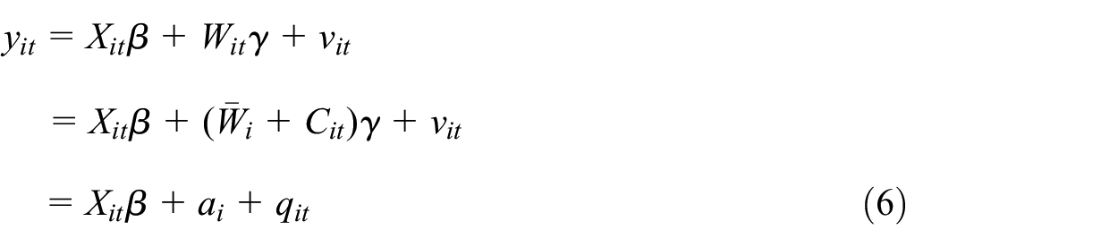
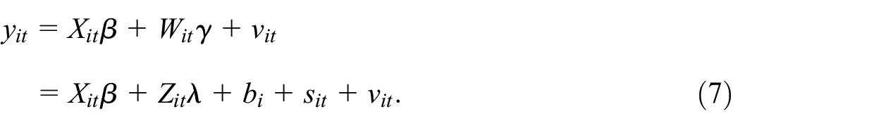
Instead of enhancing the set of observable variables, one can exploit the availability of longitudinal information, that is, panel data, to mitigate the bias from the omission of W. y, X, and Z are observed in periods t = 1, …, T with T ≥ 2 and observations are denoted as y_it, X_it, and Z_it, respectively, for units i = 1, … N. W₁ is assumed to be observed in one period only and W₂ is never observed. We consider a fixed effects (FE) model:

y_{it} = X_{it} β + a_{i} + q_{it}

with a_i + q_it = u_it. a_i is assumed to be time-invariant (the so-called fixed effect) and q_it is a time-varying error. We choose the FE model because it allows for arbitrary correlations between X and a. A more flexible specification of the individual effect would be a model with individual specific slope parameters (Wooldridge 2010, 11.7.2) but we focus here on the classical model for brevity. The FE estimator only consistently estimates β if E(q_it|X_i, a_i) = 0 with X_i = (X_i₁, …, X_iT), but neither γ₍₁₎ nor γ₍₂₎ are estimated as W₁ is not available for more than one period and W₂ is unavailable. Whether β is consistently estimated depends on the relationship between W and X because

\begin{matrix} y_{it} = X_{it} β + W_{it} γ + v_{it} \\ = X_{it} β + ({\bar{W}}_{i} + C_{it}) γ + v_{it} \\ = X_{it} β + a_{i} + q_{it} \end{matrix}

(6)

with ${\bar{W}}_{i}$ = $\sum_{t = 1}^{T} \frac{1}{T}$ W_it, C_it = W_it -- ${\bar{W}}_{i}$ , and q_it = C_itγ + v_it. a_i therefore corresponds to the time-constant part of W_itγ, which is not only the time-constant variables in W but also the time average of the time-varying components of W. E(C_itγ|X_i, ${\bar{W}}_{i}$ γ) = 0 is required for consistent estimation using a FE panel data model provided that v is idiosyncratic. It is also insightful to consider the role of Z when used in the FE model. As discussed above, Wγ can be expressed as a linear combination of the Z plus a measurement error. In terms of the panel model this is W_itγ = Z_itλ + b_i + s_it. This linear projection decomposes the measurement error into a time-constant part (b_i) and a time-varying part (s_it). Then, for the main model we have

\begin{matrix} y_{it} = X_{it} β + W_{it} γ + v_{it} \\ = X_{it} β + Z_{it} λ + b_{i} + s_{it} + v_{it} . \end{matrix}

(7)

In order to consistently estimate β by means of a FE model, b_i is allowed to be correlated with X_it and Z_it, but we need E(s_it|X_i, Z_i, b_i) = 0 and E(v_it|X_i, Z_i, b_i) = 0 with Z_i = (Z′_i1, …, Z_iT )′. The latter is again satisfied if Z does not play a role in the population model. The former, however, requires some discussion. b_i captures all time-constant features of W which are not being absorbed by Z. The more of the time-varying information of W is captured by Z, the smaller is s_it. If the time-varying information in Z_it is related to the time-varying part of W_it, s_it is smaller in size than C_itγ. Then the inconsistency of the estimated β compared to model Equation (6) is smaller. If the measurement error is time-constant, that is, s_it = 0, the FE estimator for model Equation (7) is consistent (Wooldridge 2010). A roughly time-constant measurement error (i.e., s_it $\approx 0$ ) is not implausible in applications with Z_it being proxies.

2.5. Validity Testing

The availability of W₁ makes it possible to get ideas of how usually omitted variables are related to Z. In particular, one can estimate the strength of the relationship between W₁γ₍₁₎ and Z. This shows which of the Z variables are related to unobservables and how much the variation in Z can explain the variation in W₁γ₍₁₎. A high R² would point to small measurement errors. One can also test restrictions required for Z being a set of valid proxy variables, however, valid inference requires that a model without the omitted W₂ can be consistently estimated, that is, W₂ is uncorrelated with all included variables. Testable restrictions are E(W₁γ₍₁₎|X, Z) = E(W₁γ₍₁₎|Z) and E(y|X, W₁, Z) = E(y|X, W₁), which have been motivated above. However, any correlations between (X, Z) and W₂ invalidate the inference.

Once panel models Equations (6) and (7) have been estimated, one can relate the estimated FE to W₁ and Z in a cross-sectional model. It is shown that a = $\bar{W}$ γ in model Equation (6) and b = Wγ − Zλ − s in model Equation (7). However, given that W₁ is observed in one period only, the following linear projections are suggested:

\hat{a} = W_{1} ρ + d

(8)

\hat{b} + Z \hat{λ} = W_{1} ϑ + f,

(9)

With d and f being unobserved and uncorrelated with W₁ (E(d) = E(f) = 0), the dependent variables in these models are estimated components of panel models Equations (6) and (7) designed to control for omitted W. These regressions serve two purposes: first, to assess the linear partial relationship between components of W₁ and dependent variables, indicating which components are partially controlled for. Second, the R² of these models indicates the extent to which variation in W₁ explains variation in the components controlling for W. A low R² suggests that panel models mainly control for information not in W₁ and Z (i.e., information in W₂), favoring a panel analysis with a reduced regressor set over an expanded cross-sectional analysis. Conversely, a high R² suggests that the FEs capture little time-constant information from W₂, indicating that FE panel analysis may not control for much beyond the contents of W₁.

The R² of models Equations (8) and (9) increase with L₁ and can approach one when L₁ approaches L, although in applications it is expected to stay below one because L₁ < L. Moreover, there are normally time-varying components in W₁ in Equation (8), and there is no perfect correlation between the time-varying components in Z and the time-varying components in W₁ in Equation (9), which both lead to a R² < 1 in the respective models.

Simple regression-based tests of endogeneity of X and Z can also be conducted post-FE estimation. Regressing $\hat{a}$ or $\hat{b}$ on X or (X, Z), respectively, identifies any significant relationships indicating partial correlations between FEs and observables, leading to inconsistent OLS estimates for β. These tests also identify variables or groups with these patterns.

Another route to tackle estimation biases due to omitted variables is to use instrumental variable estimation approaches, where the instrumental variables need to satisfy some validity conditions. In Supplement S.II, we present validity tests of these restrictions in models Equations (2) and (4) when W₁, $\hat{a}$ or $\hat{b}$ are available.

3. Linked Administrative and Survey Data

We use the “Integrated Employment Biographies” (IEB) of the Institute for Employment Research (IAB). The IEB are linked administrative labor market data from Germany encompassing socio-demographic characteristics and detailed employment history data of all German workers once employed in a job subject to social insurance contributions since 1975. Although the IEB covers the entire population of contributors to the social insurance system, it does not include the self-employed, lifetime civil servants, and individuals who were never economically active. In total, it contains around 85% of the total working population. Due to confidentiality reasons, the full IEB are not being made accessible for research, but the “Sample of Integrated Labour Market Biographies” (SIAB), a 2% random sample of the IEB with a reduced variable set. We augment the SIAB by linking it with survey data from the household panel study “Labour Market and Social Security” (PASS), aiming to understand the living conditions of unemployment benefit recipients. The resulting linked dataset, known as “PASS survey data linked to administrative data of the IAB” (PASS-ADIAB), is accessible through the Research Data Center (FDZ) of the IAB (Antoni and Bethmann 2014). Table 1 shows key characteristics of the underlying data products and their relationship. To facilitate comparative analysis, we narrow our sample to individuals aged 16 to 64 who participated in the fifth wave of the PASS survey in 2011, resulting in approximately 9,700 individuals. Our sample combines variables from the restricted IEB data available in the SIAB (X), generated work history variables (Z), and additional survey-based variables from PASS (W₁).

Table 1.

Structure of Underlying Official Data Products.

Product name	Size	IEB variables	SIAB variables (X)	PASS survey variables (W₁)
Integrated Employment Biographies (IEB)	100% of the population*	x	x
Sample of Integrated Labour Market Biographies (SIAB)	2% of IEB		x
Panel Study “Labour Market and Social Security” linked with IEB (PASS-ADIAB)	0.03% of IEB		x	x

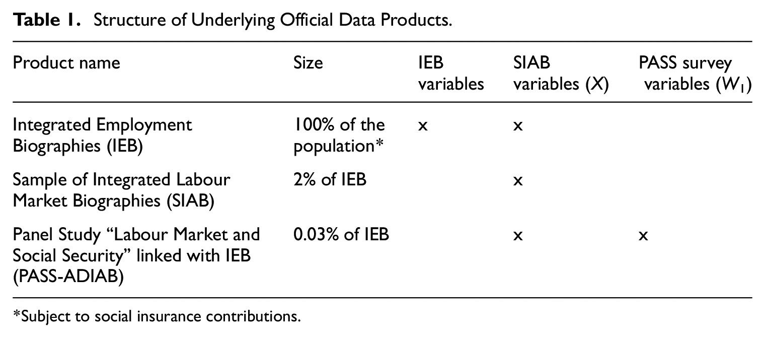
Subject to social insurance contributions.

4. Empirical Analysis

Our empirical analysis exceeds standard sensitivity analysis by applying the theoretical frameworks of Section 2 to the data on X, Z, and W₁ of Section 3. Our analysis provides insights into the role of Z, the ability of the different approaches to control for parts of Wγ, and tests for evidence of endogeneity in X and Z. We focus on linear regression models with different dependent variables: a wage regression and a linear probability model for transitions from unemployment to employment. The remainder of this section presents the results for the wage model, while the transition model outcomes are given in Supplement S.III.

Our sample for the wage regression comprises 2,435 individuals observed for at least three years in the administrative data during employment. The dependent variable (y) represents the logarithmized average daily gross wage at the time of the interview, while X includes socio-demographic and employment-related variables such as gender, age, trainee status, education, nationality, and industrial sector. In addition to these variables, we include unemployment-related register dummies, such as the receipt of unemployment insurance benefits (ALG I) and means-tested unemployment benefits (ALG II), as regressors. The W₁ variables are extracted from linked PASS data, where we select those reflecting personality traits and attitudes (Big Five), job search behavior, working hours, and social factors. The Big Five variables are used to model personality (for reviews, see John and Srivastava (1999) and McCrae and Costa (1999)). These variables are regularly included in regression analyses to account for the omission of motivation and work attitudes (Heineck and Anger 2010; Mueller and Plug 2006; Nyos and Pons 2005). As a preliminary step, we apply the LASSO and elastic net methods to identify relevant W₁ variables in model Equation (5) so that irrelevant variables in W₁ can be dropped (see Supplement S.I). Although our set of W₁ contains important factors, there are likely still omitted variables in W₂. Z consists of variables related to previous work experience, tenure, and prior unemployment experiences, serving as proxy variables. Table S6 in supplement S.IV contains the complete list of variables X, Z, and W₁ used in the wage regressions, along with their descriptive statistics.

We start by applying OLS to linear models for E(y|X), E(y|X, Z), E(y|X, W₁), and E(y|X, Z, W₁), which we denote as W.A-W.D. Table 2 presents the main estimation results for these models, while the coefficients on W₁ are reported in Table S7 in Supplement S.IV. The R² increases progressively from Model W.A to W.D, indicating the contribution of variables in explaining variation in the dependent variable. All Z and most X variables are statistically significant in models W.B and W.D., which points to sufficiently low correlations between Z and X. ${\hat{β}}_{j}$ vary considerably across the models, suggesting potential omitted variable bias and motivating the use of our approaches.

Table 2.

Wage Regression: Dependent Variable log(wage).

	W.A E(y\|X) coef. (SE)	W.B E(y\|X, Z) coef. (SE)	W.C E(y\|X, W₁) coef. (SE)	W.D E(y\|X, Z, W₁) coef. (SE)	W.E E(y_it\|X_it) coef. (SE)	W.F E(y_it\|X_it, Z_it) coef. (SE)
Gender (male = 1)	0.499*** (0.026)	0.443*** (0.024)	0.174*** (0.027)	0.148*** (0.026)	6.537* (3.564)	6.199* (3.498)
Age	0.006*** (0.001)	−0.001 (0.001)	0.011*** (0.001)	0.002 (0.001)	−0.055 (0.084)	−0.047 (0.082)
Dummy: trainee	−0.437 (0.369)	−0.342 (0.305)	−0.628** (0.285)	−0.518** (0.246)	−0.494*** (0.166)	−0.515*** (0.164)
Missing information on education	−0.528*** (0.163)	−0.438*** (0.154)	−0.394*** (0.141)	−0.300* (0.154)	0.060 (0.180)	0.055 (0.175)
No formal degree	−0.264** (0.117)	−0.215** (0.107)	−0.146 (0.090)	−0.112 (0.081)	−0.053 (0.146)	−0.040 (0.141)
Vocational training	0.030 (0.113)	−0.008 (0.103)	0.045 (0.085)	0.022 (0.076)	0.062 (0.133)	0.080 (0.127)
Higher education	0.522*** (0.117)	0.483*** (0.107)	0.434*** (0.088)	0.417*** (0.079)	0.050 (0.130)	0.056 (0.125)
Dummy: German nationality	0.030 (0.058)	−0.057 (0.055)	0.001 (0.048)	−0.072 (0.045)	−0.048 (0.130)	−0.030 (0.127)
Agriculture	−0.627*** (0.097)	−0.443*** (0.093)	−0.558*** (0.077)	−0.404*** (0.080)	−0.189 (0.561)	−0.174 (0.561)
Hotel and restaurant	−0.543*** (0.076)	−0.368*** (0.074)	−0.571*** (0.063)	−0.436*** (0.059)	−0.309 (0.200)	−0.328* (0.197)
Construction	−0.310*** (0.055)	−0.211*** (0.053)	−0.284*** (0.049)	−0.200*** (0.047)	0.139 (0.155)	0.130 (0.155)
Trade	−0.249*** (0.038)	−0.175*** (0.035)	−0.193*** (0.034)	−0.135*** (0.031)	−0.025 (0.087)	−0.022 (0.086)
Services	−0.232*** (0.034)	−0.124*** (0.032)	−0.198*** (0.032)	−0.115*** (0.030)	−0.108* (0.064)	−0.115* (0.063)
Education and social health	−0.136*** (0.037)	−0.054 (0.035)	−0.092*** (0.032)	−0.033 (0.030)	−0.066 (0.101)	−0.073 (0.099)
Public institutions	0.082* (0.045)	0.070 (0.044)	0.086** (0.037)	0.076** (0.036)	0.158 (0.179)	0.153 (0.177)
Other sectors	−0.083 (0.074)	−0.010 (0.061)	−0.015 (0.062)	0.038	−0.514**	−0.502** (0.218)
				(0.050)	(0.226)
Tenure (in years)		0.019*** (0.002)		0.018*** (0.002)		0.005 (0.006)
Share of working experience over total observation time		0.217*** (0.047)		0.118*** (0.043)		−0.123 (0.106)
Additional working experience (in years)		0.011*** (0.002)		0.013*** (0.002)		0.008 (0.007)
Dummy: unemployment history in the past		−0.492*** (0.032)		−0.427*** (0.029)		0.101 (0.145)
Constant	3.770*** (0.131)	4.200*** (0.125)	2.506*** (0.189)	2.996*** (0.178)
N	2,435	2,435	2,435	2,435	3 × 2,435	3 × 2,435
R ²	.319	.412	.502	.570	.997	.997

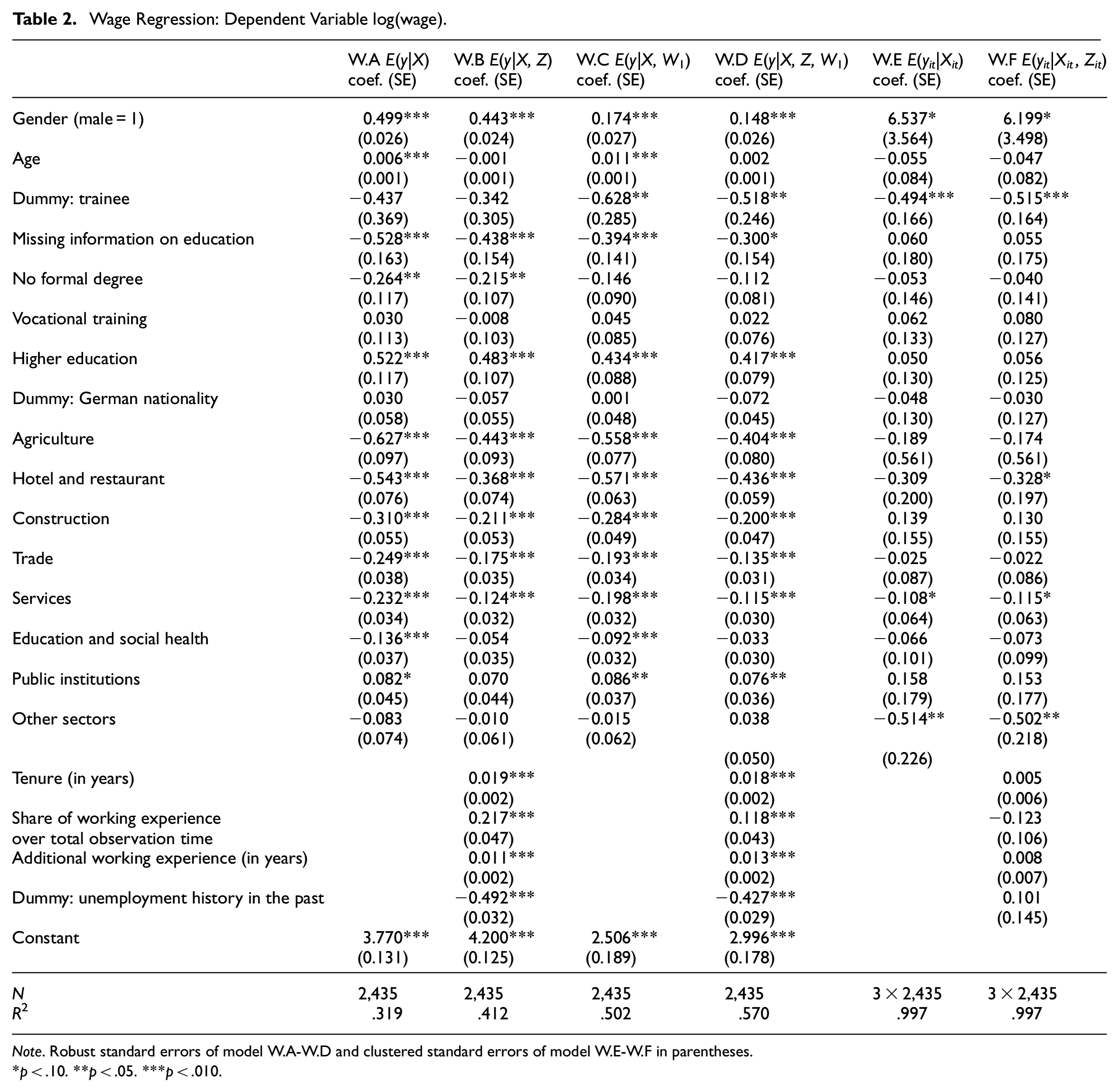
Note. Robust standard errors of model W.A-W.D and clustered standard errors of model W.E-W.F in parentheses.

*p < .10. **p < .05. ***p < .010.

The coefficients on several components of X, such as gender and higher education, change monotonically from Models W.A to W.D. This could be interpreted as an improvement of the estimates and a reduction in the omitted variable bias as the model R² increases. As outlined in Section 2, however, there is no theoretical foundation that this is always true. For some X, such as vocational training and nationality, the change is small and not statistically significant. For other variables in X, such as trainee, the coefficients do not change significantly but they gain in precision and become statistically significant. As all Z variables are individually significant in Model W.D, the restriction E(y|X, W₁, Z) = E(y|X, W₁) is violated. It can be seen from Table 3 that all but one component of Z are individually significant in the linear projection on $W_{1} {\hat{γ}}_{(1)}$ . This suggests that there is a statistical partial relationship between the linear combination of Z and the linear combination of W. However, the R² of only 0.04 points to that the variation in Z only very little explains the variation in $W_{1} \hat{γ}$ and therefore Z are poor proxies for W₁. This is also confirmed by a rejection of the restriction E(W₁γ₍₁₎|X, Z) = E(W₁γ₍₁₎|Z) with a p-value of virtually 0 using a heteroskedasticity robust F-test. Moreover, the coefficients on Z are mainly unchanged between Models W.B and W.D., which also suggests that the endogeneity of Z is not removed by adding W₁. If anything, these observations suggest that the Z variables are either components of W₂ or they are proxies for components in W₂. This would be in line with the increase in the R² when we go from Model W.C to W.D.

Table 3.

Wage Regression: Test Restrictions for Z Being Feasible Proxy Variables.

	$E (W_{1} {\hat{Y}}_{(1)} \| Z)$ coef. (SE)
Tenure (in years)	−0.000 (0.001)
Share of working experience over total observation time	0.241*** (0.028)
Additional working experience (in years)	−0.006*** (0.001)
Dummy: unemployment history in the past	−0.175*** (0.019)
N	2,435
R ²	.042

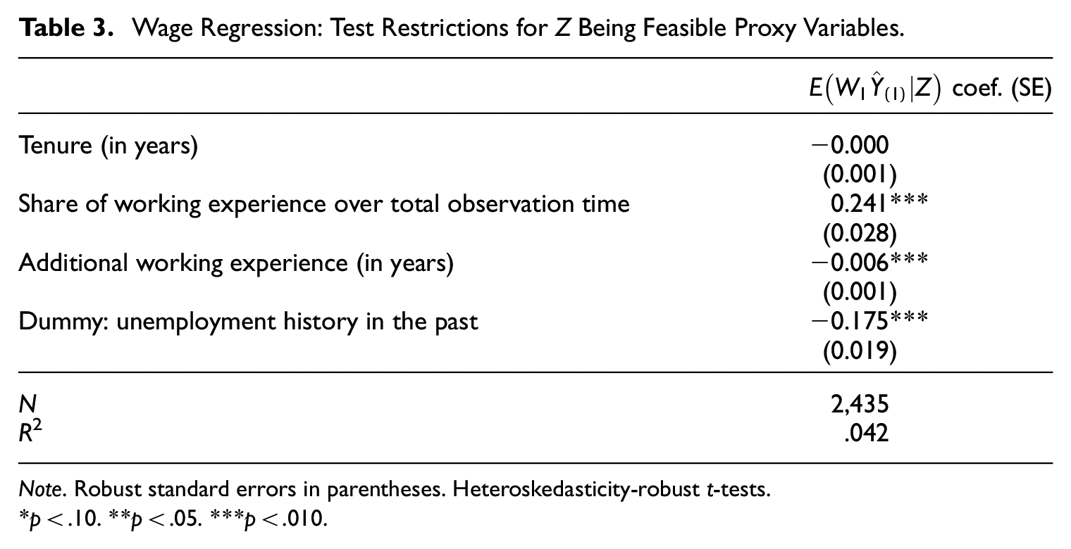
Note. Robust standard errors in parentheses. Heteroskedasticity-robust t-tests.

*p < .10. **p < .05. ***p < .010.

In order to shed more light on the role of W₁ and Z in the previous models, we estimate panel data regression Equation (6) and (7) with three periods for the same individuals as for the other models. We include period interactions for all regressors and only report the coefficients for the period that is used in the cross sectional models. In order to obtain coefficients on the time-constant variables, we estimate a dummy variable regression model with 2,435 individual specific dummy variables. The results—without the estimated a—are displayed in Table 2 as Models W.E and W.F, respectively. It is evident that the coefficients on several of the X and Z variables change considerably when using a panel model that allows for correlation between (X, Z) and the time-constant part of the error. This points to violations of the stronger assumptions of cross sectional models. For example, the coefficient on higher education drops sharply from 0.483 in Model W.B to 0.056 in Model W.F. A similar pattern can be observed for several of the business sectors, while other previously strongly significant coefficients become weak or insignificant in the panel analysis (e.g., gender). The multicollinearity pattern driving this result is briefly discussed at the end of this subsection. But there are also variables, such as trainee, for which precision increases. The coefficients on the Z variables decrease in magnitude and these variables become considerably less individually significant. A robust test whether the components of Z are jointly significant in Model W.F has a p-value of .704. This observation and given that the R² of Model W.F is not higher than that of Model W.E suggest that Z does not additionally contribute to the model. The relevance of Z in Models W.B and W.D is therefore more likely due to correlation with W₂ rather than because Z directly belongs to the population model.

In the following we shed light on two more questions: First, to what extent do the variables in W₁ explain the variation of the estimated part of the panel model that is supposed to capture the omitted W? Second, to what extent are the estimated FEs statistically related to the included X and Z? Any relationship suggests endogeneity of the latter in a cross sectional regression.

Table 4 displays the results of the linear projections of W₁ on the estimated components of the panel models that capture the unobserved W as given by Equations (8) and (9) for the cross sectional data. In the case of model Equation (6) this is simply the estimated FEs $\hat{a}$ . In the case of model Equation (7), this is the estimated FE plus the estimated component related to Z, that is, $\hat{b} + Z \hat{λ}$ . The estimated coefficients are from the panel regressions. Given that the two regressions in Table 4 have different dependent variables with different variation, the estimated coefficients and the R² are not directly comparable. However, they show that the variation in W₁ explains around one third of the variation of the dependent variables. They also show that a number of W₁ variables are partially related to the dependent variables. This is evidence of panel models effectively controlling for information in W₁ without directly using it. However, the remaining 2/3 of the variation must be due to W₂. This suggests that the panel models also effectively control for additional unobservables. To find out which other omitted variables belong to W₂, one could link additional variables to the data set and check how they contribute to the model.

Table 4.

The Statistical Relationship Between the Estimated Component of the Panel Model That Controls for Omitted W and the Observable W_1.

	$E (\hat{a} \| W_{1})$ coef. (SE)	$E (\hat{b} + Z \hat{λ} \| W_{1})$ coef. (SE)
Big Five: I am rather cautious, reserved	0.036 (0.047)	0.029 (0.057)
Big Five: I tend to criticize people	0.000 (0.041)	−0.013 (0.051)
Big Five: I attend to all my assignments with precision	0.044 (0.066)	0.045 (0.080)
Big Five: I have versatile interests	−0.132** (0.060)	−0.171** (0.073)
Big Five: I am inspirable and can inspire other people	0.027 (0.052)	0.032 (0.064)
Big Five: I easily trust in people and believe in the good in humans	0.070* (0.041)	0.094* (0.050)
Big Five: I tend to be lazy	−0.203*** (0.043)	−0.250*** (0.053)
Big Five: I am profound and like to think about things	−0.115** (0.045)	−0.139** (0.055)
Big Five: I am rather quiet, introverted	−0.292*** (0.046)	−0.375*** (0.056)
Big Five: I can act cold and distant	0.004 (0.040)	0.017 (0.049)
Big Five: I am industrious and work hard	0.200*** (0.076)	0.282*** (0.092)
Big Five: I worry a lot	0.225*** (0.041)	0.291*** (0.051)
Big Five: I have a vivid imagination and have a lot of phantasy	−0.188*** (0.052)	−0.225*** (0.063)
Big Five: I am outgoing and like company	−0.005 (0.054)	0.021 (0.066)
Big Five: I can be gruff and repellend toward other people	−0.117*** (0.043)	−0.140*** (0.053)
Big Five: I make plans and carry them out	−0.025 (0.057)	−0.038 (0.070)
Big Five: I easily get nervous and insecure	0.141*** (0.048)	0.200*** (0.058)
Big Five: I treasure artistic and aesthetic impressions	0.219*** (0.047)	0.248*** (0.057)
Big Five: I am not very interested in art	−0.152*** (0.044)	−0.176*** (0.053)
Dummy: satisfied with one’s life in general	0.389*** (0.142)	0.410** (0.173)
Dummy: was looking for a new job	−0.458*** (0.165)	−0.402** (0.202)
Dummy: was looking for an additional job	−0.708* (0.379)	−0.808* (0.463)
Dummy: was looking for a new and an additional job	0.170 (0.881)	0.402 (1.078)
Strength of connection to place of residence	−0.031 (0.046)	−0.033 (0.057)
Frequency of misunderstandings, tensions, or conflicts	−0.108** (0.049)	−0.168*** (0.059)
Number of children in total (within and outside the household)	0.212*** (0.056)	0.090 (0.068)
Number of children in household	0.295*** (0.084)	0.415*** (0.103)
Dummy: none of parents has a HE degree	0.056 (0.092)	0.019 (0.112)
Dummy: one parent has a HE degree	0.032 (0.173)	−0.016 (0.212)
Current contract working time, total, without mini-job	−0.042*** (0.008)	−0.055*** (0.010)
Current actual working time, main occupation, without mini-job	−0.074*** (0.014)	−0.095*** (0.017)
Current actual working time, total, without mini-job	0.024* (0.014)	0.029* (0.017)
Dummy: none of parents with migrational background	−0.369** (0.182)	−0.314 (0.223)
Size of household	−0.753*** (0.064)	−0.844*** (0.078)
Constant	9.482*** (0.639)	9.667*** (0.782)
N	2,435	2,435
R ²	.327	.334

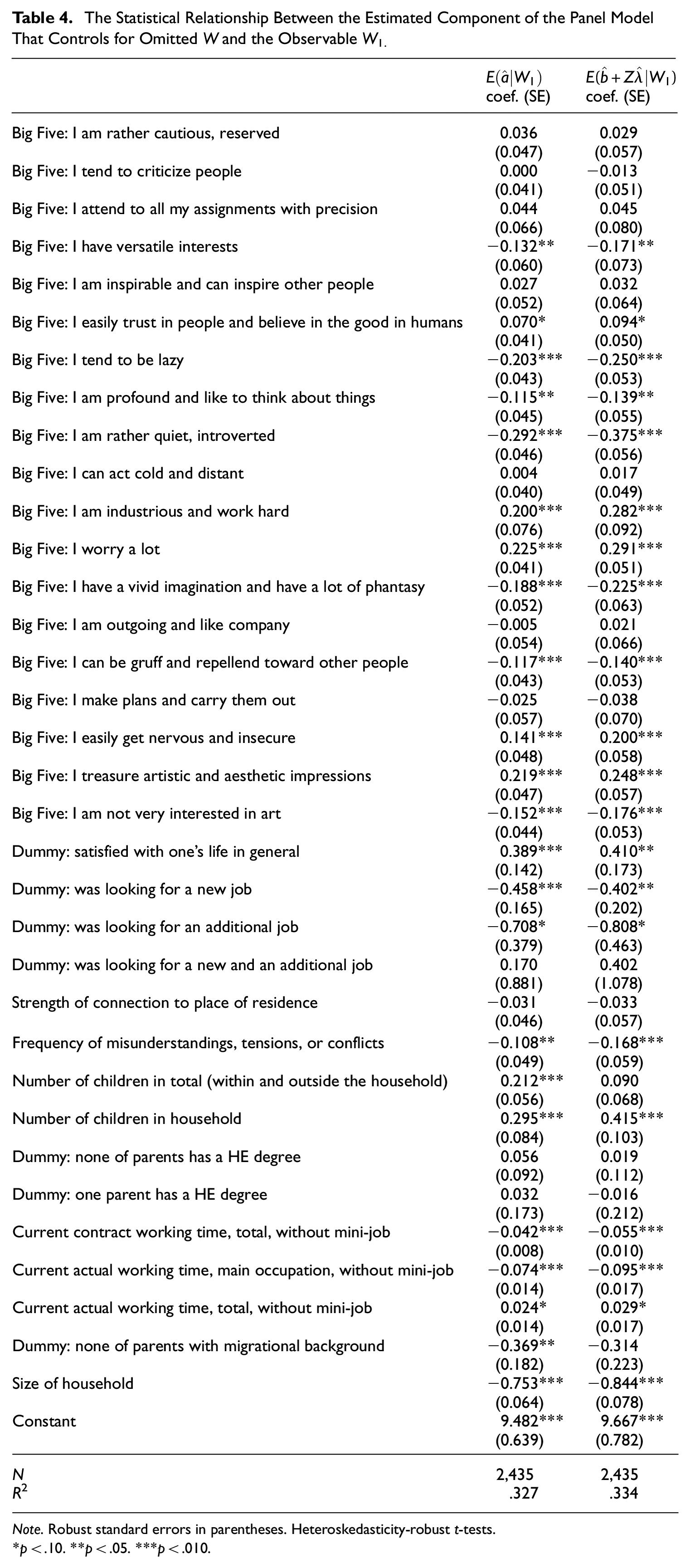
Note. Robust standard errors in parentheses. Heteroskedasticity-robust t-tests.

*p < .10. **p < .05. ***p < .010.

Table 5 reports the results for regressions of the estimated FEs from the panel analysis on the included regressors in the two models using the cross sectional data. It is apparent that a large number of the coefficients differ significantly from 0. This points to partial correlations between FEs and regressors and thus to endogeneity of the latter in the cross sectional models of Table 2. This means there is significant bias in many of the estimated coefficients of the cross sectional models W.A and W.B in Table 2. The large values of the R² for the two models in Table 5 reveal that the included regressors nearly entirely explain the variation in estimated FEs. This causes a strong multicollinearity pattern between some of the variables in the panel models of Table 2, which is reflected by the partly huge standard errors in Models W.E and W.F., for example, for the coefficient on gender. A solution to mitigate this pattern would be to use information from additional periods but this would be an unbalanced panel as individuals do not always work.

Table 5.

Wage Regression: Regression Based Endogeneity Test for Components of X and Z.

	$E (\hat{a} \| X)$ coef. (SE)	$E (\hat{b} \| X, Z)$ coef. (SE)
Gender (male = 1)	−4.867*** (0.026)	−6.249*** (0.024)
Age	0.060*** (0.001)	0.034*** (0.001)
Dummy: trainee	−0.150 (0.375)	−0.033 (0.299)
Missing information on education	−0.582*** (0.158)	−0.483*** (0.155)
No formal degree	−0.188* (0.107)	−0.126 (0.098)
Vocational training	−0.050 (0.103)	−0.082 (0.094)
Higher education	0.329*** (0.106)	0.304*** (0.097)
Dummy: German nationality	0.066 (0.059)	−0.037 (0.055)
Agriculture	−0.473*** (0.094)	−0.285*** (0.095)
Hotel and restaurant	−0.132 (0.080)	0.056 (0.075)
Construction	−0.285*** (0.059)	−0.179*** (0.058)
Trade	−0.147*** (0.039)	−0.076** (0.036)
Services	−0.145*** (0.035)	−0.030 (0.033)
Education and social health	−0.185*** (0.037)	−0.102*** (0.034)
Public institutions	−0.192*** (0.045)	−0.196*** (0.044)
Other sectors	0.223*** (0.080)	0.293*** (0.066)
Tenure (in years)		0.017*** (0.002)
Share of working experience over total observation time		0.327*** (0.048)
Additional working experience (in years)		0.004* (0.002)
Dummy: unemployment history in the past		−0.479*** (0.034)
Constant	3.735*** (0.124)	4.172*** (0.120)
N	2,435	2,435
R ²	.954	.974

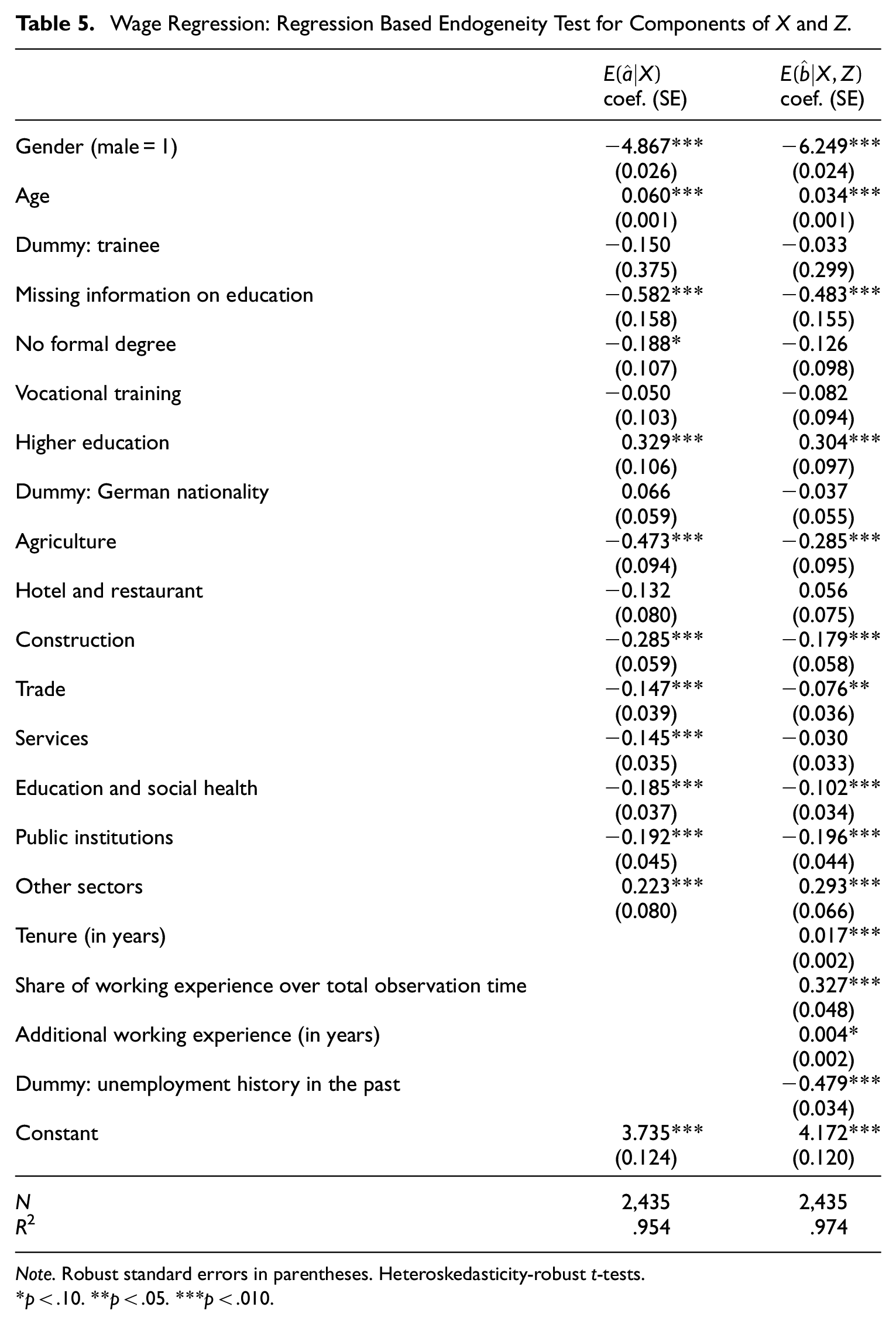
Note. Robust standard errors in parentheses. Heteroskedasticity-robust t-tests.

*p < .10. **p < .05. ***p < .010.

5. Summary and Discussion

This paper presents a unified framework for various approaches to mitigate omitted variable bias in linear regression analysis. We elucidate the mechanisms influencing the magnitude of the bias and explore the relationship between different models with distinct sets of regressors or unobserved effects. Although the theory does not provide a universally applicable model ranking, our empirical analysis sheds some light on how these approaches compare in practice.

In our application, we identify substantial omitted variable bias for several variables in the wage regression. Incorporating work history and survey variables contributes to reducing omitted variable bias. Notably, socio-demographic variables tend to align more closely with results from panel analysis as more variables are included in the model, suggesting convergence toward the values obtained from comprehensive panel data models. Utilizing panel data reveals the presence of omitted variable bias in cross-sectional results, indicating that panel analysis captures relevant unobservable components more effectively than an expanded set of regressors at a single time point. Analysis based solely on administrative data additionally benefits from higher precision due to larger sample size when survey-based variables are only available for a smaller (random) sample. Our findings also suggest that work history variables can serve as proxies for certain unobservable variables in the wage model. We advise researchers to utilize panel data whenever available, as it offers the best prospects for capturing the largest share of unobserved variables.

Our results are not only pertinent to empirical researchers but also to data providers. Given cost and data confidentiality considerations, data providers strive to supply the maximum amount of relevant information while minimizing irrelevant data. Our findings underscore the value of longitudinal information from administrative data, which contributes more substantially to the analysis than the addition of survey variables. Our findings suggest that data producers should consider making panel data based on administrative sources available and restrict surveys to variables that are required for the analysis itself but not available from administrative sources. Since panel models can capture at least partly W, the set of X that is made available to users should be also determined by data confidentiality aspects.

Supplemental Material

sj-docx-1-jof-10.1177_0282423X241312644 – Supplemental material for On Omitted Variables, Proxies, and Unobserved Effects in Empirical Regression Analysis

Supplemental material, sj-docx-1-jof-10.1177_0282423X241312644 for On Omitted Variables, Proxies, and Unobserved Effects in Empirical Regression Analysis by Shihan Du, Ralf Andreas Wilke and Pia Homrighausen in Journal of Official Statistics

Footnotes

Acknowledgements

We are grateful to the DIM unit of the IAB for providing the data, to Arne Bethmann for his support with the PASS data, and to Lisbeth La Cour and Giovanni Mellace for their valuable feedback on an earlier draft. We thank the guest editor and the three reviewers for their detailed comments and insightful feedback.

Funding

The author(s) received no financial support for the research, authorship, and or publication of this article.

ORCID iDs

Shihan Du

Ralf Andreas Wilke

Pia Homrighausen

Supplemental Material

Supplemental material for this article is available online.

Received: April 2023

Accepted: December 2024

References

Antoni

Bethmann

2014. “PASS-Befragungsdaten verknüpft mit administrativen Daten des IAB (PASS-ADIAB) 1975–2011.” FDZ-Datenreport, 03/2014, Nürnberg.

Arni

Caliendo

Künn

Mahlstedt

2014. “Predicting the Risk of Long-Term Unemployment: What Can We Learn from Personality Traits, Beliefs and Other Behavioral Variables?”Working Paper, Potsdam.

Baptista

Lima

Preto

M. T.

2012. “How Former Business Owners Fare in the Labor Market? Job Assignment and Earnings.” European Economic Review 56 (2): 263–76. DOI: https://doi.org/10.1016/j.euroecorev.2011.08.004.

Berka

Humer

Moser

Lenk

Rechta

Schwerer

2012. “Combination of Evidence from Multiple Administrative Data Sources: Quality Assessment of the Austrian Register-Based Census 2011.” Statistica Neerlandica 66 (1): 18–33. DOI: https://doi.org/10.1111/j.1467-9574.2011.00506.x.

Biewen

Fitzenberger

Osikominu

Paul

2014. “The Effectiveness of Public-Sponsored Training Revisited: The Importance of Data and Methodological Choices.” Journal of Labor Economics 32 (4): 837–97. DOI: https://doi.org/10.1086/677233.

Bollinger

C. R.

Minier

2015. “On the Robustness of Coefficient Estimates to the Inclusion of Proxy Variables.” Journal of Econometric Methods 4: 101–22. DOI: https://doi.org/10.1515/jem-2012-0008.

Caliendo

Mahlstedt

Mitknik

O. A.

2014. “Unobservable, but Unimportant? The Influence of Personality Traits (and Other Usually Unobserved Variables) for the Evaluation of Labor Market Policies.” IZA Discussion Paper No. 8337, IZA Bonn.

de Wolf

P. P.

Van der Laan

Zult

2019. “Connecting Correction Methods for Linkage Error in Capture-Recapture.” Journal of Official Statistics 35 (3): 577–97. DOI: https://doi.org/10.2478/jos-2019-0024.

Di Consiglio

Tuoto

2015. “Coverage Evaluation on Probabilistically Linked Data.” Journal of Official Statistics 31 (3): 415–29. DOI: https://doi.org/10.1515/jos-2015-0025.

10.

Dlugosz

Mammen

Wilke

R. A.

2017. “Generalized Partially Linear Regression with Misclassified Data and an Application to Labour Market Transitions.” Computational Statistics & Data Analysis 110: 145–59. DOI: https://doi.org/10.1016/j.csda.2017.01.003.

11.

Fernández-Kranz

Rodríguez-Planas

2011. “The Part-Time Pay Penalty in a Segmented Labor Market.” Labour Economics 18 (5): 591–606. DOI: https://doi.org/10.1016/j.labeco.2011.01.001.

12.

Gelbach

2016. “When Do Covariates Matter? And Which Ones, and How Much?” Journal of Labor Economics 34: 509–43. DOI: https://doi.org/10.1086/683668.

13.

Hand

D. J.

2018. “Statistical Challenges of Administrative and Transaction Data.” Journal of the Royal Statistical Society: Series A (Statistics in Society) 181 (3): 555–605. DOI: https://doi.org/10.1111/rssa.12315.

14.

Harron

Dibben

Boyd

, et al. 2017. “Challenges in Administrative Data Linkage for Research.” Big Data & Society 4 (2): 2053951717745678. DOI: https://doi.org/10.1177/2053951717745678.

15.

Heineck

Anger

2010. “The Returns to Cognitive Abilities and Personality Traits in Germany.” Labour Economics 17: 535–46. DOI: https://doi.org/10.1016/j.labeco.2009.06.001.

16.

John

O. P.

Srivastava

1999. “The Big-Five Trait Taxonomy: History, Measurement, and Theoretical Perspectives.” In Handbook of Personality: Theory and Research, edited by Pervin

L. A.

John

O. P.

, 102–138. New York: Guilford Press.

17.

Kauhanen

Napari

2012. “Career and Wage Dynamics: Evidence from Linked Employer-Employee Data.” In Research in Labor Economics, Vol. 36, edited by Polachek

S. W.

Tatsiramos

, 1–30. Bingley: Emerald Group Publishing Limited.

18.

Lechner

Wunsch

2013. “Sensitivity of Matching-Based Program Evaluations to the Availability of Control Variables.” Labour Economics 21: 111–21. DOI: https://doi.org/10.1016/j.labeco.2013.01.004.

19.

Lubotsky

Wittenberg

2006. “Interpretation of Regressions with Multiple Proxies.” Review of Economics and Statistics 88: 549–62. DOI: https://doi.org/10.1162/rest.88.3.549.

20.

McCrae

Costa

P. T.

1999. “A Five-Factor Theory of Personality.” In J. S. Wiggins (Ed.), The Five-Factor Model of Personality: Theoretical Perspectives, Vol. 2. New York, NY: Guilford Press.

21.

Mueller

Plug

E. J. S.

2006. “Estimating the Effect of Personality on Male and Female Earnings.” Industrial & Labor Relations Review 60: 3–22. DOI: https://doi.org/10.1177/001979390606000101.

22.

Nyos

Pons

2005. “The Effects of Personality on Earnings.” Journal of Economic Psychology 26: 363–84. DOI: https://doi.org/10.1016/j.joep.2004.07.001.

23.

Oberski

D. L.

Kirchner

Eckman

Kreuter

2017. “Evaluating the Quality of Survey and Administrative Data with Generalized Multitrait-Multimethod Models.” Journal of the American Statistical Association 112 (520): 1477–89. DOI: https://doi.org/10.1080/01621459.2017.1302338.

24.

Oster

2019. “Unobservable Selection and Coefficient Stability.” Journal of Business and Economic Statistics 37: 187–204. DOI: https://doi.org/10.1080/07350015.2016.1227711.

25.

Schnetzer

Astleithner

Cetkovic

Humer

Lenk

Moser

2015. “Quality Assessment of Imputations in Administrative Data.” Journal of Official Statistics 31 (2): 231–47. DOI: https://doi.org/10.1515/jos-2015-0015.

26.

Wooldridge

J. M.

2010. Econometric Analysis of Cross Section and Panel Data. 2nd ed. Cambridge, MA: MIT Press.

27.

Yildiz

Smith

P. W.

2015. “Models for Combining Aggregate-Level Administrative Data in the Absence of a Traditional Census.” Journal of Official Statistics 31 (3): 431–51. DOI: https://doi.org/10.1515/jos-2015-0026.

28.

Zhang

L. C.

2012. “Topics of Statistical Theory for Register-Based Statistics and Data Integration.” Statistica Neerlandica 66 (1): 41–63. DOI: https://doi.org/10.1111/j.1467-9574.2011.00508.x.

Supplementary Material

Please find the following supplemental material available below.

For Open Access articles published under a Creative Commons License, all supplemental material carries the same license as the article it is associated with.

For non-Open Access articles published, all supplemental material carries a non-exclusive license, and permission requests for re-use of supplemental material or any part of supplemental material shall be sent directly to the copyright owner as specified in the copyright notice associated with the article.

0.00 MB

0.11 MB

On Omitted Variables,Proxies,and Unobserved Effects in Empirical Regression Analysis

Abstract

Keywords

1. Introduction

2. The Model

2.1. Omitted Variable Bias

2.2. Proxy Variables

2.3. Survey Data

2.4. Panel Data

2.5. Validity Testing

3. Linked Administrative and Survey Data

4. Empirical Analysis

5. Summary and Discussion

Supplemental Material

sj-docx-1-jof-10.1177_0282423X241312644 – Supplemental material for On Omitted Variables, Proxies, and Unobserved Effects in Empirical Regression Analysis

Footnotes

Acknowledgements

Funding

ORCID iDs

Supplemental Material

References

Supplementary Material