Sage Journals: Discover world-class research

Abstract

The rising cost of survey data collection is an ongoing concern. Cost predictions can be used to make more informed decisions about allocating resources efficiently during data collection. However, telephone surveys typically do not provide a direct measure of case-level costs. As an alternative, I propose using the number of call attempts as a proxy cost indicator. Most previous studies have focused on logistic regression and linear regression for cost estimation. This study advocates time-to-event models for predicting survey costs. To improve cost predictions, I dynamically adjust predictive models for future call attempts required until an interview or refusal during the nonresponse follow up. This update is achieved by fitting models on the training set for cases that are still unresolved as of a particular number of call attempts. This approach accommodates additional paradata collected on each case up to that point. I use data from the Health and Retirement Study to evaluate the ability of alternative models to predict the number of future call attempts required until interview or refusal. These models include a baseline model with only time-invariant covariates (discrete time hazard regression), accelerated failure time regression, survival trees, and Bayesian additive regression trees within the framework of accelerated failure time models.

Keywords

survey cost responsive survey design machine learning paradata

1. Introduction

To address the issue of declining response rates and rising costs of data collection (Williams and Brick 2018), researchers have begun exploring responsive survey design (RSD) to improve the efficiency of data collection (Groves and Heeringa 2006). RSD is an evidence-based approach that uses incoming data to make near real-time design decisions that aim to reduce survey costs or errors. Groves (2005) posits that survey costs and errors are interconnected, meaning that increasing one reduces the other. Precise cost predictions can help survey managers to make better decisions about allocating field resources. However, there have been only a few studies that have directly examined methods for improving real-time cost prediction (Coffey 2020; Wagner et al. 2020).

Cost predictions are a critical input to the decision rules in RSD (Schouten et al. 2018; Wagner et al. 2023). Survey managers will make better cost-error tradeoff decisions if they know which types of participants that are relatively hard to recruit and understand how different they are with respect to the survey variables from easy-to-recruit participants. In the RSD context, accurate cost predictions help to reduce both survey errors and costs. However, inaccurate cost predictions would misinform these decisions, resulting in budget overruns, missing targets for the number of interviews and failing to meet statistical goals.

A direct measure of case-level costs is not typically available in telephone surveys that are not centralized. In practice, it is easier for interviewers to report the total hours they worked in a given time period (e.g., a day or a week) than to record the total minutes spent on each call attempt. To predict costs at the case level, Wagner et al. (2023) proposed a cost prediction algorithm that estimates cumulative interviewer hours out to twenty-one call attempts. They used a discrete time hazard model to estimate propensity scores for future call attempts, including only time-invariant covariates in the model. They computed the estimated interviewer hours for each call attempt as a weighted average of several propensity scores for different call attempt outcomes, with weights being the estimated interviewer hours for those outcomes. They then adjusted the interviewer hours for each future call attempt by the estimated probability of not being interviewed at that call attempt. However, their cost predictions were not effective in clearly differentiating high-cost cases from low-cost cases, and can be further improved by accounting for incoming data (e.g., outcomes of previous call attempts).

An alternative approach to improving cost predictions is to explore proxy cost indicators. One such indicator is the number of call attempts, which can serve as a strong proxy for the cost at the case level. While the number of call attempts misses the certain aspects of interviewer hours that reflect the total costs of a case, the number of call attempts considers case difficulty and has been used as a survey cost indicator to improve the efficiency of data collection. For example, Groves and Heeringa (2006) set a maximum number of call attempts for a design phase at ten to fourteen attempts in the National Survey of Family Growth (NSFG). They found that it was possible to achieve additional cost savings without compromising the quality of key estimates by moving some cases into the next phase of data collection early.

To improve the efficiency of call scheduling, Durrant et al. (2015, 2017) predicted the number of call attempts required to finalize a case using data from the UK longitudinal household survey, Understanding Society. In their study, more than six call attempts made at a sampled address were considered unproductive. Identifying cases that were more likely to require more than six call attempts early in the data collection process could save costs. They dichotomized the number of call attempts required to finalization into a long call sequence length (more than six call attempts) or a short call sequence length (up to six call attempts), and used logistic regression to model the probability of a short call sequence length.

The modeling approach used by Durrant et al. had two important limitations. First, dichotomizing a continuous dependent variable has undesirable analytical consequences. For example, overall statistical power is compromised as the variation of the continuous variable on either side of the cutoff point is ignored (Selvin 1987), and the magnitudes of regression coefficients and their associated test statistics are affected by the cutoff point chosen (Ragland 1992). Second, their model failed to account for right censoring. For example, a short call sequence length can occur when an interviewer stops effort on a case that would require more call attempts to finalize. Estimates based on methods that ignore right censoring, such as excluding right-censored cases or assuming that an event occurred at the last observation for each censored case, can be biased (Leung et al. 1997; Tuma and Hannan 1979). Inaccurate predictions of future call attempts can reduce the effectiveness of RSD. If an expensive case is misclassified as inexpensive, insufficient resources will be allocated to it, potentially resulting in nonresponse. Conversely, if an inexpensive case is misclassified as expensive, more resources than necessary will be allocated to it, affecting data collection productivity.

Time-to-event models have been used to predict survey design quantities. Coffey (2020) used a hurdle model to predict the time lag between the day of the first attempt and the day of the first contact as a measure of case difficulty. The hurdle modeling approach handles mixtures of zero and non-zero outcomes and allows cases to be contacted on day 0. However, in practice, only predictors that are available on day 0 can be used in the hurdle model, as later information is not yet available. Once a case has been attempted but not yet contacted on day 0, the hurdle portion of the model is no longer necessary and the time to first contact can be re-estimated using newly collected information from the day of the first attempt onwards.

Updating predictions for time-to-event data with time-varying covariates is known as dynamic prediction in survival analysis (van Houwelingen and Putter 2011). In the clinical context, the prognosis of a patient can be updated using repeated measurements of biomarkers. Dynamic prediction may produce more accurate predictions than static prediction since it accounts for both covariates with time-varying effects and time-varying covariates. As an example of dynamic prediction in the survey methodology context, Mittereder and West (2022) used a dynamic survival model (an extended form of the Cox survival model) that accounts for page-varying covariates and coefficients to predict breakoff on the next page of a web survey.

Recent advancements in machine learning have provided survey researchers and social scientists with a new set of analytic tools for making predictions (Buskirk and Kirchner 2020). With the increase in computational power and the improvement of prediction algorithms, it is now possible to analyze large-scale and complex data in a timely manner. In particular, survey researchers have started using tree-based models to predict survey design quantities, since these models can identify complex interactions and nonlinear relationships. For example, Kern et al. (2019, 2023) used tree-based models to improve predictions of panel nonresponse, and found that ensemble methods (e.g., random forests, extreme gradient boosting, and extra trees) performed the best. However, in comparison, penalized logistic regression was found to outperform predictions based on a single decision tree, likely due to overfitting with the single decision tree in the training set. Tree-based models have also been applied to predicting interviewer hours in field work. Wagner et al. (2020) compared the ability of two Bayesian Additive Regression Trees (BART) models and a multilevel regression model to predict the interviewer hours in a given week using data from the National Survey of Family Growth. They found that the random intercept BART model accounting for interviewer effects produced the most accurate predictions. These studies highlight the potential of tree-based models in predicting survey design quantities.

In this study, I aim to evaluate the ability of dynamic time-to-event models to improve predictions for future call attempts required until an interview or refusal. I consider the “real” cost of a case, where the cost limit has been reached once the case is finalized by an interview or a final refusal. Therefore, the predictive models for comparison include a baseline model with only time-invariant covariates (discrete time hazard regression), accelerated failure time (AFT) regression, survival trees, and Bayesian Additive Regression Trees within the framework of accelerated failure time (AFT-BART) models. As more paradata are collected on each case at later call attempts, I examine how the quality of predictions changes over different cutoff points. A cutoff point can be used for setting a design phase of data collection, and the number of call attempts made on sample cases is considered the cutoff point in this context. This study addresses the following research questions:

RQ1. How should time-varying paradata best be used in time-to-event models (i.e., multiple measurements at multiple time points, or the last observed measurement at the most recent time point)?

RQ2. How accurately can alternative time-to-event models predict the number of future call attempts until an interview or refusal?

RQ3. Does the best type of time-to-event model for making predictions change over different cutoff points?

2. Data

2.1. The Health and Retirement Study

The data for this study come from the 2014, 2016, and 2018 waves of the Health and Retirement Study (HRS). The HRS is a nationally representative longitudinal survey of United States (U.S.) adults aged 51 and older (Fisher and Ryan 2018; Sonnega et al. 2014). A new cohort of HRS participants aged 51 to 56 is added every six years using an area probability sampling design (e.g., in 1998, 2004, 2010, 2016, etc.). Age-eligible individuals and their spouses, regardless of age, are interviewed to obtain both household- and individual-level data. The HRS measures the changes in health and economic conditions among older U.S. adults over time.

The HRS used a mixed-mode design to collect data in the 2016 and 2018 waves, where face-to-face (FTF) and telephone were the two main modes of data collection (the web mode was introduced as an alternative mode of data collection in the 2018 wave). For panel members over the age of 80, the HRS offered FTF interviewing in both waves. Beginning with the 2006 wave, a random half of the sample received an enhanced FTF interview with additional physical and biomarker measures and psychosocial questions. The other half completes only a core interview, usually by telephone. The HRS alternates modes for these two random half samples each wave. In other words, HRS participants receive enhanced FTF interviews at four-year intervals beginning in 2006/2008.

In the 2016 wave, the HRS added the Late Baby Boomer (LBB; born in 1960–1965) cohort to the study. Most sample cases in the baseline interview were interviewed by FTF. Therefore, fifty new recruits (most likely spouses) out of 8,484 cases were interviewed by telephone in the 2016 wave. For the LBB cohort, a random half received an enhanced FTF interview and the other half received a core interview by FTF in the 2016 wave. In the 2018 wave, a panel member below the age of 80 would receive a core interview by telephone if he/she was assigned to an enhanced FTF interview in the 2016 wave, and a panel member would receive an enhanced FTF interview if he/she was assigned to a regular FTF core interview in the 2016 wave. This study aims to predict case-level costs in the telephone component of the 2018 HRS. The predictions of case-level costs in an FTF interview would need to consider travel costs, which would require a separate study. I used data from the HRS sample cases that were assigned to the telephone mode in the 2016 wave to train predictive models, and then evaluated predictions for the HRS sample cases that were assigned to the telephone mode in the 2018 wave.

Interviewers for the HRS are employed and trained by the Survey Research Center at the University of Michigan. To minimize attrition, HRS staff maintain contact with the participants by sending holiday cards and newsletters, and interviewers establish and maintain rapport with the HRS participants. In advance of the interview, HRS staff first send a letter to each HRS survey participant as a pre-notification and then follow up by telephone. Panel respondents are prepaid a token of appreciation of $80 in their precontact mailing, while baseline respondents (newly screened into the HRS) are paid a token of appreciation of $100 after completing the interview.

In the telephone mode, the HRS does not have a case delivery system that assigns cases to interviewers. Instead, each interviewer receives a list of cases to attempt and can decide when to attempt a case and which case to attempt first. Because the HRS interview requires one to two hours to complete, an interviewer usually makes an appointment with a sample case for the interview. Interviewers may also attempt a case as many times as they need. This call scheduling setting adds a further dose of uncertainty for modeling the number of call attempts until an interview or refusal. An optimal call scheduling minimizes the number of call attempts required to resolve a case, ultimately reducing survey costs (Brick et al. 1996; Weeks et al. 1987). However, identifying the optimal call scheduling falls beyond the scope of this study. In this study, I assume that call scheduling can be partially explained by the covariates described in Subsection 2.3. It is worth mentioning that predictions of future call attempts would be less accurate if call scheduling depends on unobserved data. For example, voicemail messages might indicate when a case is available for contact and can be used to improve the contact rate in the future. However, these messages may not be captured in call record data and thus cannot be used in a predictive model.

Table 1 presents the sample sizes and censored cases of the 2016 and 2018 waves, as well as the mean, median, minimum, and maximum call attempts to resolve a case by an interview or refusal in each corresponding wave. Compared to the 2016 wave, the 2018 wave had more censored cases and a larger median number of call attempts required until an interview or refusal. The shift in the median call attempts to resolve a case indicates that the difficulty of resolving a case has increased over time. While, the means were almost the same in the two waves (the mean was 16.7 for the 2016 wave when the upper limit of call attempts was set to 137).

Table 1.

Descriptive Statistics in the Telephone Component of the 2016 and 2018 Waves of the HRS.

Wave	Sample size	Censored cases (%)	Mean^a (SE)	Median^b	Min	Max
2016	8,484	237 (2.7)	16.8 (0.3)	7	1	178
2018	8,327	1,070 (12.8)	16.8 (0.2)	10	1	137

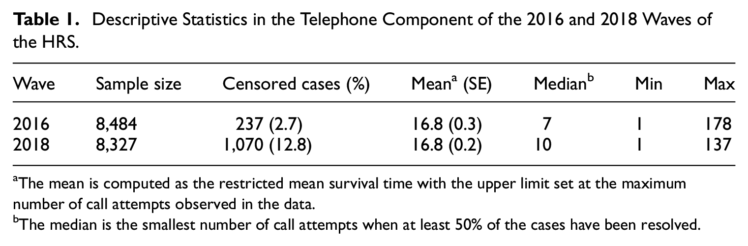
The mean is computed as the restricted mean survival time with the upper limit set at the maximum number of call attempts observed in the data.

The median is the smallest number of call attempts when at least 50% of the cases have been resolved.

2.2. Future Call Attempts Required Until an Interview or Refusal

In this study, the outcome variable of interest is the number of future call attempts until a case either completes the interview or refuses to participate in the interview, denoted by $T$ . Some cases may never reach either of these events (also known as right censoring). If a case is right censored by a stopping rule, the number of call attempts required until an interview or refusal $T$ for this case is not observable, and recorded survey costs are lower than real survey costs. Let $C$ be the potential censoring number of call attempts and $Y = \min (T, C)$ be the observed final call attempt number. The censoring indicator is denoted as $δ = I (T \geq C)$ (i.e., $δ = 1$ if a case is censored and otherwise $δ = 0$ ). I classify a case as censored if the outcome of the final call attempt falls within one of the following five categories: tracking exhausted (when interviewers give up finding a sample member), never answered, incomplete interview, mail/email/text auto return, and stopping rule.

Let $S (t)$ denote the survival function for a case that is unresolved from call attempt 0 to the $t$ th call attempt. Figure 1 shows the survival distributions for cases that were attempted by twenty-six or fewer call attempts in the telephone component of the 2016 and 2018 waves of the HRS. The Kaplan-Meier curves for all cases in the telephone component of both waves are shown in Appendix B.1. The prediction of the number of future call attempts required until an interview or refusal may change for a case that is still unresolved after the $ω$ th call attempt. However, the survival function $S (t)$ estimated at call attempt 0 does not reflect how the prediction changes over time. Thus, I rely on the conditional survival function $CS (t | ω) = \frac{S (ω + t)}{S (ω)}$ for $t \geq 0$ , which can be interpreted as the conditional probability of being unresolved at the $(ω + t)$ th call attempt, given that the case is still unresolved at the $ω$ th call attempt.

Figure 1.

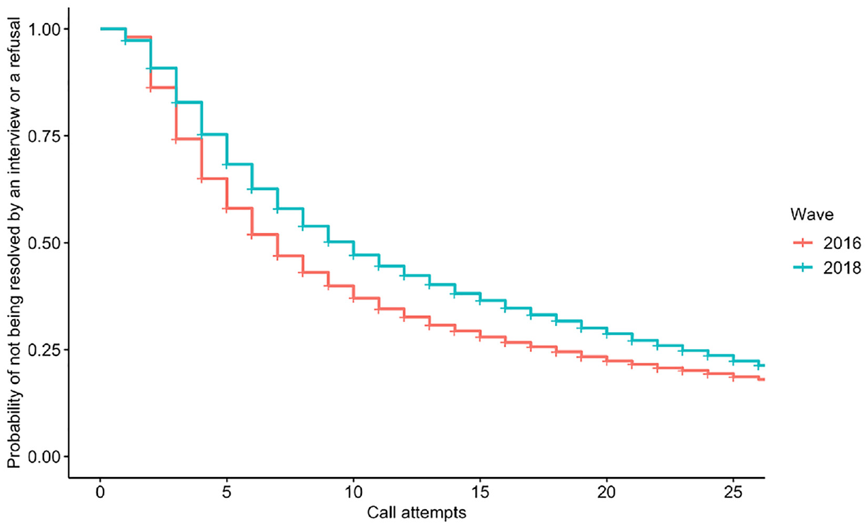
Kaplan-Meier curves for cases that were attempted by twenty-six or fewer call attempts in the telephone component of the 2016 and 2018 waves of the HRS.

To address RQ3, I select three cutoff points, $ω = (3, 6, 15)$ , to compare the ability of alternative time-to-event models in predicting the number of future call attempts required until an interview or refusal. These cutoff points correspond to when 26%, 48%, and 72% of the cases were resolved in the 2016 wave. These cutoff points were as close as possible to the quartiles (25%, 50%, and 75%). From studying these three specific cutoff points, I hope to draw a broad conclusion about the best cost prediction model that can be extended to other cutoff points. In practice, the number of future call attempts to resolve a case can be estimated at any cutoff point, but the best cutoff point should be aligned with the optimal timing of intervention.

In this study, I focus on the median number of future call attempts required until an interview or refusal, since the median is insensitive to outliers and the target distribution is right-skewed. If the censoring is not severe, the median number of call attempts required until an interview or refusal can be empirically estimated using a nonparametric method, such as the Kaplan-Meier estimator. In cases where censoring is severe, parametric methods can extrapolate beyond the observed data by taking advantage of an appropriate parametric distribution. The predictions for future call attempts also consider covariates, which will be described in more detail below.

2.3. Covariates

A description of the covariates used in this study can be found in Appendix B.2. These covariates can be grouped into four categories:

a. Socio-demographic variables

b. HRS survey variables from the previous wave

c. Survey response status in the previous wave of data collection

d. Call record data from the current wave

To reduce the risk of selection bias, I include nonrespondents in the training set. The details about missing information for each variable can be found in Appendix B.2. I imputed missing data in the socio-demographic variables and the 2014 and 2016 HRS survey variables using a sequential regression approach (Raghunathan et al. 2001). The missing data were imputed in IVEware (Raghunathan et al. 2002). Specifically, function limitations (with a bound of 0–23) and age were treated as continuous variables, educational attainment was treated as a count variable, and all the other variables were treated as categorical variables. The final imputed dataset was created after five cycles of sequential imputation. I treated those new recruits in the 2016 wave as nonrespondents in the 2014 wave, and their survey variables in the 2014 were imputed based on sequential imputation; survey variables across waves were highly correlated. In practice, the values of survey variables from the previous wave for new recruits can either be set to a separate category or be estimated by data that are available prior to data collection (e.g., Census Bureau’s Planning Database, sampling frame data, and commercial data). I leave the topic of exploring alternative data sources for future work.

2.3.1. Outcomes of Previous Call Attempts

One focus of this study is how to incorporate the outcomes of previous call attempts into the models (RQ1). Call attempt outcomes are obtained from call record data. The outcome of each call attempt for an unresolved case by definition does not include an interview or a final refusal, so that the outcome of a previous call attempt is recoded into one of four categories:

contact—soft refusal,

contact—appointment,

contact—others (e.g., callbacks), and

no contact.

To obtain the first three call attempt outcomes defined above, an interviewer has to successfully contact the case. Specifically, I examine the use of the last observed measurement and multiple measurements for the outcomes of previous call attempts for each of the cutoff points (i.e., 3, 6, and 15). For the last observed measurement, the predictive information mainly comes from the outcome of the most recent call attempt at the cutoff point. In contrast, I allow all previous call attempts to provide predictive information of the future number of call attempts when using multiple measurements. It is worth mentioning that Durrant et al. (2017) used the multiple measurements in their models to predict the number of call attempts required to finalize a case.

2.3.1.1. Last Observed Measurement

I create a measurement of the outcome of the most recent call attempt, as determined by the selected cutoff point, to classify cases into one of five categories:

contact—soft refusal,

contact—appointment,

contact—others (e.g., callbacks),

no contact, and

never contact.

In this variable, category 4 (no contact) indicates that a case was contacted before but not at the most recent call attempt, and category 5 (never contact) indicates that a case has never been contacted at the cutoff point. The value of this summary measure is updated after each call attempt. The last observed measurement approach can be extended to include outcomes of multiple previous call attempts. Such an extension might perform better than the last observed measurement approach. To explore this alternative approach, future work needs to first examine the temporal correlation between the current call attempt outcome and its previous call attempt outcomes.

2.3.1.2. Multiple Measurements

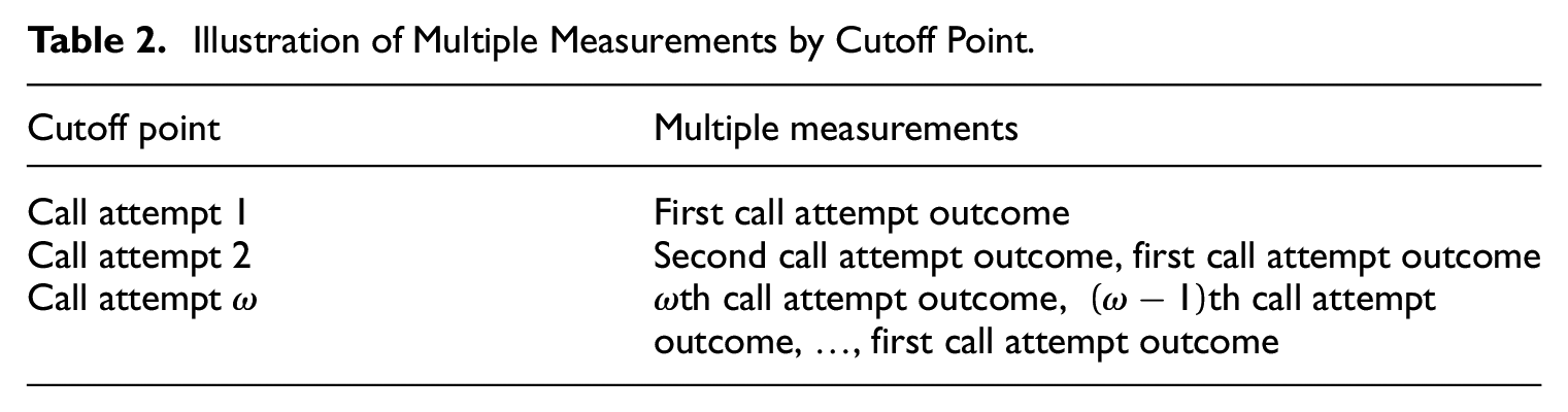
I treat the outcome of each previous call attempt as a separate covariate with the four categories mentioned above (i.e., contact—soft refusal, contact—appointment, contact—others, and no contact). The number of these covariates is equal to the count of previous of call attempts at the cutoff point. Table 2 shows an example of multiple measurements for cutoff point 1, 2, and $ω$ .

Table 2.

Illustration of Multiple Measurements by Cutoff Point.

Cutoff point	Multiple measurements
Call attempt 1	First call attempt outcome
Call attempt 2	Second call attempt outcome, first call attempt outcome
Call attempt $ω$	$ω$ th call attempt outcome, $(ω - 1)$ th call attempt outcome, …, first call attempt outcome

3. Modeling Approach

3.1. Time-to-Event Models

I consider both the discrete time and continuous time approaches of time-to-event models in cost predictions. The discrete time approach includes the discrete time hazard model (Singer and Willett 1993), which requires data at the call attempt level. The discrete time hazard model is a natural choice for predicting the number of future call attempts required until an interview or refusal. As a point of comparison, I consider this modeling approach as a “baseline” against which to compare the alternative models (i.e., continuous time approach) described below. To obtain the estimated median number of future call attempts to resolve a case, I can use the discrete time hazard model to make predictions for a horizon of future call attempts. In this study, I used a horizon of up to 200 future call attempts to ensure that the estimated median number of future call attempts was identifiable for each unresolved case. Fitting the model with the outcome of the previous call attempt to the training set is feasible, but the outcome of the previous call attempt is not available for any future call attempt beyond the next one in the test set. Details about the training and test sets for the discrete time hazard model are shown in Appendix B.3. Specifying an appropriate imputation model for future call attempt outcomes is outside the scope of the current work. Thus, I exclude this variable in the discrete time hazard model. This decision might compromise the predictive performance, since time-varying paradata may contain useful information for prediction (Durrant and D’Arrigo 2014; Mittereder and West 2022).

Alternatively, I treat the number of future call attempts required for an interview or a refusal as a continuous outcome. This type of model requires pre-specifying the parametric distribution of the outcome variable. I evaluated the empirical distribution of the number of future call attempts required until an interview or refusal in the 2016 HRS telephone component against the Poisson, Weibull, Gamma, and lognormal distributions using the fitdistrplus package (Delignette-Muller and Dutang 2015) in R. Based on the Akaike and Schwarz’s Bayesian information criteria (AIC and BIC), the lognormal distribution had the best model fit for all selected cutoff points.

The continuous time approach, requiring data at the case level, includes the lognormal accelerated failure time model (LN-AFT; Kalbfleisch and Prentice 2011), the survival tree (Therneau and Atkinson 1997), and the Bayesian Additive Regression Trees within the framework of lognormal accelerated failure time model (LN-AFT-BART; Bonato et al. 2011). The LN-AFT model is a parametric model, which has the advantage in interpretability. While, the survival tree and the LN-AFT-BART model allows for detecting complex interactions and nonlinear relationships. Particularly, the LN-AFT-BART model is a type of tree-based ensemble model that reduces the risk of overfitting. For this modeling approach, I also compare the performance of these three models that use either the multiple measurements of the outcomes of previous call attempts or the last observed measurement.

In total, I compare seven models. They are the discrete time hazard, LN-AFT with the last observed measurement, survival tree with the last observed measurement, LN-AFT-BART with the last observed measurement, LN-AFT with multiple measurements, survival tree with multiple measurements, and LN-AFT-BART with multiple measurements. For each model, I first trained the prediction models using data that are available prior to the cutoff point of the 2018 wave. Then, I made predictions of future call attempts for cases that are unresolved at the cutoff point. Predictors in the test set are also available prior to the cutoff point. This setup ensures that a survey manager can use the predictions in a real data collection. Details about the training and test sets for each model are available in Appendix B.3. The form of each model and the corresponding variables can be found in Appendix B.4 and Appendix B.2, respectively.

3.2. Evaluative Metric

To answer RQs1 to 3, I use a censoring-incorporated mean absolute error (MAE) to evaluate the performance of the alternative time-to-event models in predicting future call attempts required until an interview or refusal. The MAE measures the similarity between predictions and observations. A lower score of the MAE indicates a model with better predictive performance.

The MAE is a type of L1-loss measure. I choose the L1-loss over the L2-loss (e.g., mean squared error) because the distribution of the number of future call attempts is right skewed and the L1-loss is less sensitive to outliers. For an unresolved case with the observed number of future call attempts $t$ and the censoring indicator $δ$ , the predicted number of future call attempts is denoted by $\hat{t}$ . The MAE is given by

MAE = E [(t - \hat{t}) I_{\hat{t} < t} + (1 - δ) (\hat{t} - t) I_{\hat{t} \geq t}],

where $I$ is an indicator function.

The MAE is a scale-dependent accuracy measure, so the results can be misleading when comparing two predictions at different scales. Harrell’s concordance index (C-index; Harrell et al. 1982) is a rank-correlation measure and capable of dealing with censored data. However, comparing two C-indices is a low-power procedure because the C-index does not sufficiently reward accurate extreme predictions. Therefore, the MAE and C-index each have their own issues. To address these issues, I rescale predictions to ensure they are on the same scale as the predictions made by the baseline model. Then, I use the MAE to compare rescaled predictions made by different models. I also compute the C-index for each model to verify the MAE results (see Appendix B.8), because the C-index does not depend on rescaling. The best model should have both the lowest MAE and highest C-index.

The discrete time approach uses both resolved and unresolved cases in the training set, but the continuous time approach uses only unresolved cases. Thus, the continuous time approach would be heavily influenced by outliers (cases with a large number of call attempts to resolve) and might produce larger predictions than the discrete time approach. For comparison purposes, I rescale predictions made by the continuous time approach. I use a scaling factor that is a ratio of two predicted overall median numbers of future call attempts; the numerator is from the baseline model and the denominator is from the LN-AFT model with the last observed measurement. For each cutoff point, the scaling factor is applied to all the predictions made by the continuous time approach. Specifically, I use factors 0.91 (14/15.3), 0.80 (18/22.6), and 0.73 (29/39.6) to adjust predictions made by the LN-AFT, survival tree, and LN-AFT-BART models after call attempts 3, 6, and 15, respectively. We can also use an alternative scaling factor that is a ratio of the predicted overall median number of future call attempts from the baseline model to that of the model of interest to adjust predictions (see Appendix B.9 for more details). Future research is needed to evaluate if the improvements in these cost predictions lead to better decisions.

3.3. Implementation

All models were fitted in R. The “baseline” discrete time hazard models were fit using the glm function with a complementary log-log link function. The LN-AFT models with only main effects were fit using the survreg function in the survival package. I used the rpart function in the rpart package to implement the survival tree models and the abart function in the BART package to implement the LN-AFT-BART models. In the LN-AFT-BART models, I treated the first 500 MCMC iterations as burn-in iterations (i.e., throwing away the first 500 iterations for convergence purposes) and I kept 1,000 MCMC iterations after burn-in. The convergence diagnostics indicated that the chains converged quickly.

In the test set, the tree-based models use the best hyperparameters determined by cross-validation on the training set. Specifically, I performed ten-fold cross validation on the training set and the hyperparameters were tuned by grid search to optimize the performance of the survival trees and LN-AFT-BART models. In ten-fold cross-validation, the training set is randomly partitioned into ten equally sized subsets. The model is then trained and evaluated ten times, each time using a different subset as the test set and the remaining nine subsets as the training set. The possible values of hyperparameters are provided in Appendix B.5, and they are common values for testing. The optimal sets of hyperparameters for the survival trees and LN-AFT-BART models are shown in Appendices B.6 and B.7, respectively.

I also estimated the error bar for the MAE. I used the bootstrapping approach to estimate the 95% confidence interval of the MAE for the discrete time hazard, LN-AFT, and survival tree models. Following the bootstrap-based method, I drew 1,000 samples with replacement from the training set at each cutoff point. Each bootstrap sample had the same sample size as the training set. Then, the predictive models were built on each bootstrap sample for making predictions on the test set. In the analysis, the point estimate of the MAE for the survival tree model could be slightly below the lower bound of the 95% bootstrap confidence interval. I note that the optimal hyperparameters are only tuned for the training set but not for each bootstrap sample, and underperformance can therefore occur in the bootstrap samples. For the LN-AFT-BART models, I used the 95% credible interval from 1,000 MCMC iterations after burn-in.

4. Results

I compared the predictive performance of four types of time-to-event models by computing the MAEs based on rescaled predictions to answer RQs1 to 3 (see Figure 2). To address RQ2, I also compared the predicted and observed number of call attempts using scatter plots (see Figure 3). Table 3 provides the observed median number of future call attempts to finalization in the test set and their corresponding unscaled predictions at the three selected cutoff points.

Figure 2.

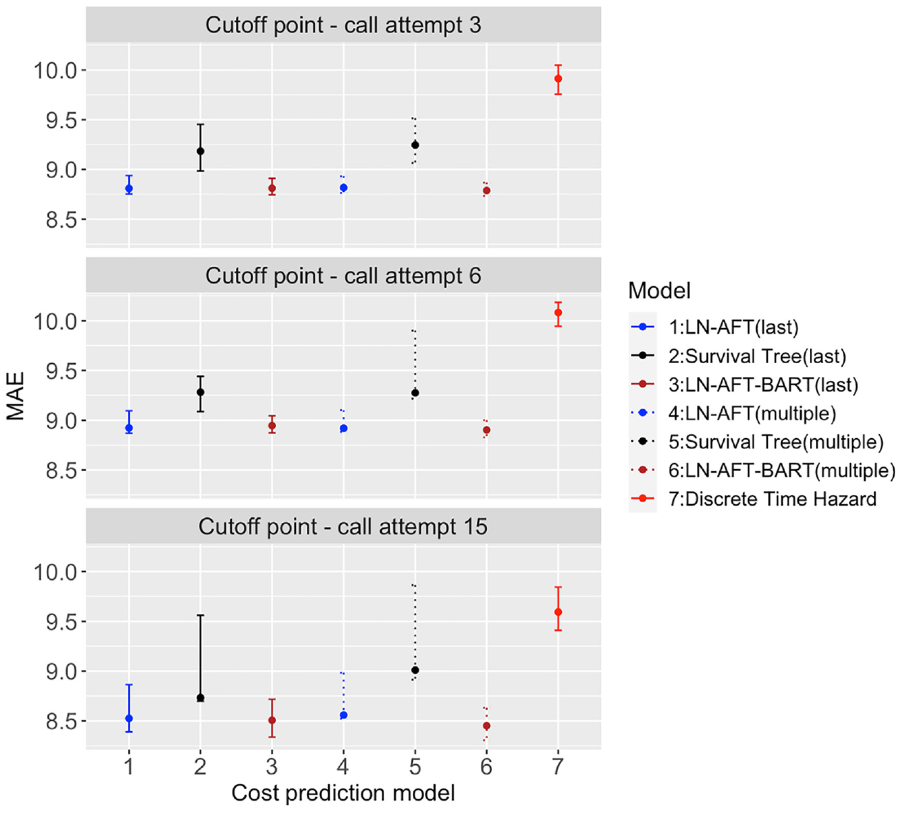
The MAEs for seven cost prediction models with 95% bootstrap or credible intervals at three cutoff points by the method of incorporating the outcomes of previous call attempts.

Figure 3.

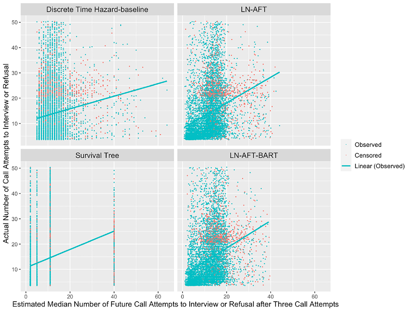
The actual number of call attempts and estimated median number of future call attempts required until an interview or refusal at call attempt 3 in the test set for discrete time hazard regression, LN-AFT (Multiple), Survival Tree (Multiple), and LN-AFT-BART (Multiple), including regression lines only for observed cases.

Table 3.

The Median Numbers of Future Call Attempts Required Until an Interview or Refusal with 95% Confidence Intervals and Their Corresponding Unadjusted Predictions with 95% Bootstrap or Credible Intervals.

Statistical method	Call attempt 3	Call attempt 6	Call attempt 15
Median (test set)	13.0 (12.0, 13.0)	19.0 (18.0, 19.0)	29.0 (29.0, 30.0)
Predictive model
LN-AFT (last)	15.4 (15.0, 15.9)	22.6 (21.6, 23.3)	39.6 (38.3, 40.6)
Survival tree (last)	15.0 (11.0, 16.0)	20.0 (18.0, 24.0)	36.0 (33.0, 38.0)
LN-AFT-BART (last)	15.6 (15.0, 16.0)	22.5 (21.6, 23.3)	39.3 (38.1, 40.6)
LN-AFT (multiple)	15.5 (15.0, 15.9)	23.2 (21.6, 23.3)	40.3 (38.4, 41.1)
Survival tree (multiple)	14.0 (11.0, 16.0)	19.0 (18.0, 25.0)	36.0 (32.0, 40.0)
LN-AFT-BART (multiple)	15.8 (15.2, 16.1)	23.2 (22.3, 23.8)	39.8 (38.5, 40.9)
Discrete time hazard	14.0 (13.0, 14.0)	18.0 (17.0, 18.0)	29.0 (29.0, 29.0)

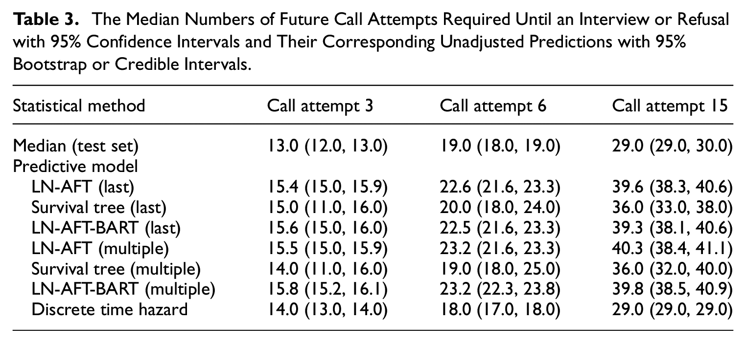
Table 3 revealed that predictions made by the continuous time approach (e.g., LN-AFT, survival tree, and LN-AFT-BART) were excessively larger than the median number of call attempts to resolve a case. Therefore, I rescaled the predictions for comparison purposes and used the C-index to verify these findings (see Appendix B.8). Appendix B.8 also shows the C-indices for two versions of the hurdle model (Coffey 2020; the hurdle part is a logistic regression model and the second part is the LN-AFT model in this study). The “current” version of the hurdle model used available data during the 2018 HRS data collection to estimate model parameters, while the “historical” version used data from the entire 2016 HRS data collection to estimate model parameters. The continuous time approach outperformed the hurdle models at each cutoff point in terms of the C-index.

Figure 2 plots MAEs for the predictive models at three cutoff points (see Appendix B.9 for similar results of MAEs using an alternative scale, where the denominator of the scaling factor is replaced by the overall median number of future call attempts based on each model). Overall, the time-to-event models that incorporated outcomes of previous call attempts significantly outperformed the baseline model, indicating strong added benefits of using the outcomes of previous call attempts in prediction, regardless of how outcomes of previous call attempts were incorporated into the predictive models. The LN-AFT-BART and LN-AFT models outperformed the survival tree model, especially after cutoff points call attempts 3 and 6. Compared to LN-AFT, the predictive performance of LN-AFT-BART was slightly better; however, the difference was not statistically significant.

I also compare the predictive performance of these models across three different cutoff points. In general, the MAEs for each of these models increased from cutoff point call attempt 3 to 6, but decreased from 6 to 15. These changes in the MAEs were not statistically significant except for the baseline model from 6 to 15. I also found that the error bar of the MAE was wider for a later cutoff point. The survival tree model had the widest error bar at each cutoff point.

At cutoff point call attempt 15, LN-AFT-BART with the multiple measurements slightly outperformed the predictive performance of LN-AFT-BART with the last observed measurement, but the improvement was not statistically significant. After fifteen call attempts, the multiple measurements method incorporates the outcomes of all fifteen call attempts into the predictive model, while the last observed measurement method only includes the outcome of the fifteenth call attempt and an additional category of never contact. Surprisingly, although the difference is not statistically significant, the survival tree model with multiple measurements had a higher value of the MAE than the survival tree model with the last observed measurement at call attempt 15. Overall, the models with the multiple measurements and their corresponding models with the last observed measurement had similar predictive performance.

Figure 3 shows four scatter plots of the actual number of call attempts versus the estimated median number of future call attempts required until an interview or refusal for unresolved cases at the cutoff point call attempt 3 in the test set. The equivalent scatter plots at the cutoff points call attempts 6 and 15 can be found in Appendices B.10 and B.11, respectively. I evaluate the accuracy of the baseline model and three alternative predictive models that used multiple measurements by visualizing their predictions. Regression lines were added to scatter plots for observed cases, and the slopes of these regression lines indicated a weak positive correlation between the actual and estimated future call attempts required until an interview or refusal. In particular, the baseline model had a noticeably flatter slope compared to others. The predictions of the discrete time hazard, LN-AFT and LN-AFT-BART models were dispersed along the x-axis. While, the survival tree model classified the unresolved cases into four different groups, resulting in four different prediction values. The number of terminal nodes in the survival tree model depends on the tuned hyperparameters. The best set of hyperparameters would achieve the optimal bias-variance tradeoff. I also noted the smallest estimated median number of future call attempts for the discrete time hazard model were larger than other models. Similar patterns were observed for the other two cutoff points and the models using the last observed measurement.

The results suggest that LN-AFT-BART and LN-AFT were consistently the two best models at different cutoff points and LN-AFT-BART had slightly better predictive performance than LN-AFT in terms of the MAE, although the difference in these two models was not statistically significant.

5. Discussion

This study examined the predictive performance of alternative dynamic time-to-event models in predicting the number of future call attempts required until an interview or refusal in the HRS. This study favors incorporating outcomes of previous call attempts into the predictive models rather than using the survey variables from the previous wave. This finding was also reported by Durrant et al. (2017). Moreover, I examined two approaches for incorporating the outcomes of previous call attempts into the predictive models. The last observed measurement and multiple measurements appear to contain similar predictive information, suggesting that predictive information mainly comes from the last observed measurement in this case. That being said, additional work on different ways to incorporate various time-varying variables could further improve the predictive performance.

This study confirms that predictive performance mainly relies on the set of covariates included in the model (Kern et al. 2023). Thus, future studies in this area should explore other covariates that have more or less predictive power of future call attempts to further boost model performance. For example, some specific circumstances (e.g., illness and temporary absence/holiday) are crucial drivers of call scheduling. These circumstances should be considered in the predictive model. These covariates might be only available at a certain time point of data collection. To address this challenge, the continuous time approach could treat them as time-varying covariates and use the most updated values of such covariates at a certain point in time. While, this modeling approach requires that these covariates are also available in the training set for model building.

I found that the MAE increased from cutoff point call attempt 3 to 6, but decreased from 6 to 15. Two competing factors may affect the accuracy of predictions for future call attempts over time. On the one hand, cases that are resolved easily (i.e., within a few call attempts) can be predicted more accurately compared to cases that require more call attempts. Once these cases are finalized, the remaining unresolved cases can be hard to predict. For example, cases with an interview appointment are more likely to be finalized at the next call attempt, but the probability of scheduling an interview appointment decreases at later call attempts. On the other hand, the predictions would get closer to the final call attempts as more call attempts are spent on a case. In other words, the remaining number of call attempts to predict decreases at a late cutoff point. As mentioned above, the MAE is a scale-dependent accuracy measure. For comparison purposes, I adjusted the predictions for the continuous time approach mentioned above. The adjusted predictions made by the continuous time approach, as well as the unadjusted predictions made by the discrete time hazard model, closely match the overall median number of future call attempts in the test set. The adjustment factor became smaller at later cutoff points, indicating outliers that require a lot of call attempts to resolve may affect the predictions for the continuous time approach, especially at a late cutoff point.

This study is not without limitations. First, I make the implicit assumption that the costs for cases within the same household (e.g., coupled households) are independent of one another. However, if one household member has been contacted, they may inform others in the household about the upcoming interview, potentially affecting the independence assumption. Second, the study only considers independent censoring and the training set has no more than 2% of cases that were censored in the training set. If censored cases are selective in the training set, one approach is to use inverse probability of censoring weighting (IPCW; Robins and Finkelstein 2000; Zhang and Schaubel 2011) to account for it. The IPCW approach assumes that there is no unmeasured confounder for censoring; otherwise, it could fail to correct for selection bias. Then, IPCW assigns different weights to each case using the inverse of the estimated probability of being censored. Third, I assume that cases with the same number of call attempts to finalization have equal costs. In reality, some call attempts may require less time and resources compared to others. Cost prediction approaches that account for variations in cost among cases with the same number of call attempts could further improve predictions.

Improving survey cost predictions is a promising research direction. I used the cost modeling approach for a survey design that allows for a large number of call attempts for nonresponse follow-up in a telephone mode. In practice, some types of call attempts take longer than others. For example, the first successful contact might need extra time for introducing the survey request. Future studies might also consider the type of future call attempts to further improve cost estimation. There are also many other types of surveys, and cost prediction models should be aligned with the survey design (i.e., fitness for use). Two important design factors for cost prediction models are the number of attempts allowed to obtain an interview and the survey mode. First, the proposed modeling approach for survey costs can be extended to surveys that set a limit on the total number of callbacks. For example, the conditional restricted mean survival time (CRMST) can be used to predict future costs for a survey with the maximum number of call attempts. The CRMST represents the average number of future attempts, and is estimated by the area under the conditional survival curve from the most recent call attempt number to the maximum call attempt number. Second, the choice of the survey mode also affects the cost structure of data collection. For example, a mail/web survey is self-administered and typically has less variability in the case-level costs. However, the travel costs vary across sampled blocks in a FTF survey.

The results presented in this study yield two suggestions for survey practitioners to improve cost predictions for informing survey decisions. First, incorporating time-varying paradata (such as outcomes of previous call attempts) into a cost prediction model would boost its performance. All the models incorporating previous call attempt outcomes demonstrated better performance compared to the baseline model, which did not consider any previous call attempt outcomes. However, paradata recorded by interviewers may be prone to measurement error (Biemer et al. 2013; Wagner et al. 2017), which could attenuate the actual association between these paradata and the number of future call attempts required to resolve a case. Thus, future research should explore the sensitivity of cost predictions to paradata at different levels of measurement error, especially for paradata that have the most impacts on predictions. Second, the LN-AFT and LN-AFT-BART models outperformed the survival tree model in terms of the MAE. The survival tree model may be susceptible to a higher level of the variance in predictions, because the predictions are only based on a single survival tree. To inform a possible range of cost predictions, the LN-AFT-BART model would be particularly useful since it allows for quantifying uncertainty.

While the advocated methodology for estimating survey costs might work best in panel studies, it is still relevant elsewhere. For example, incorporating incoming paradata into predictive models and using the LN-AFT or LN-AFT-BART model can greatly improve predictions. A cross-sectional study lacks survey variables from a previous wave, but predictors can be derived from the Census Bureau’s Planning Database, sampling frame, and existing call record data that are available for use during data collection. For a cross-sectional survey, the training set may come from a similar survey. Specifically, a repeated cross-sectional survey can use data from the previous wave to build predictive models.

The dynamic time-to-event models to predict the number of future call attempts are developed in the context of responsive survey designs. These cost predictions can be produced and monitored during data collection for intervention in real time. Future research is needed to examine if this cost prediction approach can help responsive survey designs to improve the efficiency of data collection.

Footnotes

Appendices

Acknowledgements

The author would like to thank dissertation committee chair James Wagner as well as committee members Katharine G. Abraham, Michael R. Elliott, and Brady T. West.

Author Note

This research was carried out as part of a PhD dissertation at the University of Michigan, Ann Arbor.

Funding

The author received no financial support for the research, authorship, and/or publication of this article.

ORCID iD

Xinyu Zhang

Received: November 2023

Accepted: October 2024

References

Biemer

P. P.

Chen

Wang

2013. “Using Level-of-Effort Paradata in Non-Response Adjustments with Application to Field Surveys.” Journal of the Royal Statistical Society: Series A (Statistics in Society) 176 (1): 147–68. DOI: https://doi.org/10.1111/j.1467-985X.2012.01058.x.

Bonato

Baladandayuthapani

Broom

B. M.

Sulman

E. P.

Aldape

K. D.

K. A.

2011. “Bayesian Ensemble Methods for Survival Prediction in Gene Expression Data.” Bioinformatics 27 (3): 359–67. DOI: https://doi.org/10.1093/bioinformatics/btq660.

Breiman

Friedman

J. H.

Olshen

R. A.

Stone

C. J.

1984. Classification and Regression Trees. Wadsworth. DOI: https://doi.org/10.1201/9781315139470.

Brick

J. M.

Allen

Cunningham

Maklan

1996. “Outcomes of a Calling Protocol in a Telephone Survey.”Proceedings of the Survey Research Methods Subsection of the American Statistical Association, Chicago, IL, August 4–8.

Buskirk

T. D.

Kirchner

2020. “Why Machines Matter for Survey and Social Science Researchers: Exploring Applications of Machine Learning Methods for Design, Data Collection, and Analysis.” In Big Data Meets Survey Science: A Collection of Innovative Methods, edited by Craig A. Hill, Paul P. Biemer, Trent D. Buskirk, Lilli Japec, Antje Kirchner, Stas Kolenikov, and Lars E. Lyberg, 9–62. John Wiley & Sons. DOI: https://doi.org/10.1002/9781118976357.ch1.

Chipman

H. A.

George

E. I.

McCulloch

R. E.

2010. “BART: Bayesian Additive Regression Trees.” The Annals of Applied Statistics 4 (1): 266–98. DOI: https://doi.org/10.1214/09-AOAS285.

Coffey

2020. “Bayesian Methods for Prediction of Survey Data Collection Parameters in Adaptive and Responsive Designs.” PhD thesis, University of Maryland. DOI: https://doi.org/10.13016/uemn-z6ms.

Delignette-Muller

M. L.

Dutang

2015. “fitdistrplus: An R Package for Fitting Distributions.” Journal of Statistical Software 64: 1–34. DOI: https://www.jstatsoft.org/article/view/v064i04.

Durrant

G. B.

D’Arrigo

2014. “Doorstep Interactions and Interviewer Effects on the Process Leading to Cooperation or Refusal.” Sociological Methods & Research 43 (3): 490–518. DOI: https://doi.org/10.1177/004912411452114.

10.

Durrant

G. B.

Maslovskaya

Smith

P. W.

2015. “Modeling Final Outcome and Length of Call Sequence to Improve Efficiency in Interviewer Call Scheduling.” Journal of Survey Statistics and Methodology 3 (3): 397–424. DOI: https://doi.org/10.1093/jssam/smv008.

11.

Durrant

G. B.

Maslovskaya

Smith

P. W.

2017. “Using Prior Wave Information and Paradata: Can They Help to Predict Response Outcomes and Call Sequence Length in a Longitudinal Study?” Journal of Official Statistics 33 (3): 801–33. DOI: https://doi.org/10.1515/jos-2017-0037.

12.

Fisher

G. G.

Ryan

L. H.

2018. “Overview of the Health and Retirement Study and Introduction to the Special Issue.” Work, Aging and Retirement 4 (1): 1–9. DOI: https://doi.org/10.1093/workar/wax032.

13.

Groves

R. M.

2005. Survey Errors and Survey Costs. Wiley. DOI: https://doi.org/10.1002/0471725277.

14.

Groves

R. M.

Heeringa

S. G.

2006. “Responsive Design for Household Surveys: Tools for Actively Controlling Survey Errors and Costs.” Journal of the Royal Statistical Society: Series A (Statistics in Society) 169 (3): 439–57. DOI: https://doi.org/10.1111/j.1467-985X.2006.00423.x.

15.

Harrell

F. E.

Califf

R. M.

Pryor

D. B.

Lee

K. L.

Rosati

R. A.

1982. “Evaluating the Yield of Medical Tests.” JAMA 247 (18): 2543–6. DOI: https://doi.org/10.1001/jama.1982.03320430047030.

16.

Kalbfleisch

J. D.

Prentice

R. L.

2011. The Statistical Analysis of Failure Time Data. 2nd ed. John Wiley & Sons. DOI: https://doi.org/10.1002/9781118032985.

17.

Kaplan

E. L.

Meier

1958. “Nonparametric Estimation from Incomplete Observations.” Journal of the American Statistical Association 53 (282): 457–81. DOI: https://doi.org/10.1080/01621459.1958.10501452.

18.

Kern

Klausch

Kreuter

2019. “Tree-Based Machine Learning Methods for Survey Research.” Survey Research Methods 13 (1): 73–93. DOI: https://doi.org/10.18148/srm/2019.v1i1.7395.

19.

Kern

Weiß

Kolb

J. P.

2023. “Predicting Nonresponse in Future Waves of a Probability-Based Mixed-Mode Panel with Machine Learning.” Journal of Survey Statistics and Methodology 11 (1): 100–23. DOI: https://doi.org/10.1093/jssam/smab009.

20.

Leung

K. M.

Elashoff

R. M.

Afifi

A. A.

1997. “Censoring Issues in Survival Analysis.” Annual Review of Public Health 18 (1): 83–104. DOI: https://doi.org/10.1146/annurev.publhealth.18.1.83.

21.

Mittereder

West

B. T.

2022. “A Dynamic Survival Modeling Approach to the Prediction of Web Survey Breakoff.” Journal of Survey Statistics and Methodology 10 (4): 945–78. DOI: https://doi.org/10.1093/jssam/smab015.

22.

Raghunathan

T. E.

Lepkowski

J. M.

Van Hoewyk

Solenberger

2001. “A Multivariate Technique for Multiply Imputing Missing Values Using a Sequence of Regression Models.” Survey Methodology 27 (1): 85–96.

23.

Raghunathan

T. E.

Solenberger

P. W.

Van Hoewyk

2002. IVEware: Imputation and Variance Estimation Software. Survey Methodology Program, Survey Research Center, Institute for Social Research, University of Michigan.

24.

Ragland

D. R.

1992. “Dichotomizing Continuous Outcome Variables: Dependence of the Magnitude of Association and Statistical Power on the Cutpoint.” Epidemiology 3 (5): 434–40. DOI: https://doi.org/10.1097/00001648-199209000-00009.

25.

Robins

J. M.

Finkelstein

D. M.

2000. “Correcting for Noncompliance and Dependent Censoring in an AIDS Clinical Trial with Inverse Probability of Censoring Weighted (IPCW) Log-Rank Tests.” Biometrics 56 (3): 779–88. DOI: https://doi.org/10.1111/j.0006-341x.2000.00779.x.

26.

Schouten

Mushkudiani

Shlomo

Durrant

Lundquist

Wagner

2018. “A Bayesian Analysis of Design Parameters in Survey Data Collection.” Journal of Survey Statistics and Methodology 6 (4): 431–64. DOI: https://doi.org/10.1093/jssam/smy012.

27.

Selvin

1987. “Two Issues Concerning the Analysis of Grouped Data.” European Journal of Epidemiology 3 (3): 284–7. DOI: https://doi.org/10.1007/BF00149737.

28.

Singer

J. D.

Willett

J. B.

1993. “It’s About Time: Using Discrete-Time Survival Analysis to Study Duration and the Timing of Events.” Journal of Educational Statistics 18 (2): 155–95. DOI: https://doi.org/10.2307/1165085.

29.

Sonnega

Faul

J. D.

Ofstedal

M. B.

Langa

K. M.

Phillips

J. W.

Weir

D. R.

2014. “Cohort Profile: The Health and Retirement Study (HRS).” International Journal of Epidemiology 43 (2): 576–85. DOI: https://doi.org/10.1093/ije/dyu067.

30.

Tanner

M. A.

Wong

W. H.

1987. “The Calculation of Posterior Distributions by Data Augmentation.” Journal of the American Statistical Association 82 (398): 528–40. DOI: https://doi.org/10.1080/01621459.1987.10478458.

31.

Therneau

T. M.

Atkinson

E. J.

1997. “An Introduction to Recursive Partitioning Using the RPART Routines.” Technical Report 61, Subsection of Biostatistics, Mayo Clinic, Rochester. http://stat.ethz.ch/R-manual/R-patched/library/rpart/doc/longintro.pdf (accessed November, 2023).

32.

Therneau

T. M.

Grambsch

P. M.

Fleming

T. R.

1990. “Martingale-Based Residuals for Survival Models.” Biometrika 77 (1): 147–60. DOI: https://doi.org/10.1093/biomet/77.1.147.

33.

Tuma

N. B.

Hannan

M. T.

1979. “Approaches to the Censoring Problem in Analysis of Event Histories.” Sociological Methodology 10: 209–40. DOI: https://doi.org/10.2307/270772.

34.

van Houwelingen

Putter

2011. Dynamic Prediction in Clinical Survival Analysis. CRC Press. DOI: https://doi.org/10.1201/b11311.

35.

Wagner

Olson

Edgar

2017. “The Utility of GPS Data in Assessing Interviewer Travel Behavior and Errors in Level-of-Effort Paradata.” Survey Research Methods 11 (3): 219–33. DOI: https://doi.org/10.18148/srm/2017.v11i3.6794.

36.

Wagner

West

B. T.

Elliott

M. R.

Coffey

2020. “Comparing the Ability of Regression Modeling and Bayesian Additive Regression Trees to Predict Costs in a Responsive Survey Design Context.” Journal of Official Statistics 36 (4): 907–31. DOI: https://doi.org/10.2478/jos-2020-0043.

37.

Wagner

Zhang

Elliott

M. R.

West

B. T.

Coffey

2023. “An Experimental Evaluation of a Stopping Rule Aimed at Maximizing Cost-Quality Tradeoffs in Surveys.” Journal of the Royal Statistical Society: Series A (Statistics in Society) 186 (4): 788–810. DOI: https://doi.org/10.1093/jrsssa/qnad059.

38.

Weeks

M. F.

Kulka

R. A.

Pierson

S. A.

1987. “Optimal Call Scheduling for a Telephone Survey.” Public Opinion Quarterly 51 (4): 540–9. DOI: https://doi.org/10.1086/269056.

39.

Williams

Brick

J. M.

2018. “Trends in US Face-to-Face Household Survey Nonresponse and Level of Effort.” Journal of Survey Statistics and Methodology 6: 186–211. DOI: https://doi.org/10.1093/jssam/smx019.

40.

Zhang

Schaubel

D. E.

2011. “Estimating Differences in Restricted Mean Lifetime Using Observational Data Subject to Dependent Censoring.” Biometrics 67 (3): 740–9. DOI: https://doi.org/10.1111/j.1541-0420.2010.01503.x.

Dynamic Time-to-Event Models for Future Call Attempts Required Until Interview or Refusal

Abstract

Keywords

1. Introduction

2. Data

2.1. The Health and Retirement Study

2.2. Future Call Attempts Required Until an Interview or Refusal

2.3. Covariates

2.3.1. Outcomes of Previous Call Attempts

2.3.1.1. Last Observed Measurement

2.3.1.2. Multiple Measurements

3. Modeling Approach

3.1. Time-to-Event Models

3.2. Evaluative Metric

3.3. Implementation

4. Results

5. Discussion

Footnotes

Appendices

Acknowledgements

Author Note

Funding

ORCID iD

References