
Abstract
There is a growing trend among statistical agencies to explore non-probability data sources for producing more timely and detailed statistics, while reducing costs and respondent burden. Coverage and measurement error are two issues that may be present in such data. The imperfections may be corrected using available information relating to the population of interest, such as a census or a reference probability sample. In this paper, we compare a wide range of existing methods for producing population estimates using a non-probability dataset through a simulation study based on a realistic business population. The study was conducted to examine the performance of the methods under different missingness and data quality assumptions. The results confirm the ability of the methods examined to address selection bias. When no measurement error is present in the non-probability dataset, a screening dual-frame approach for the probability sample tends to yield lower sample size and mean squared error results. The presence of measurement error and/or nonignorable missingness increases mean squared errors for estimators that depend heavily on the non-probability data. In this case, the best approach tends to be to fall back to a model-assisted estimator based on the probability sample.
1. Introduction
Probability survey samples have been, for the best part of the last century, the preferred data collection tool of statistical agencies for producing population estimates. Neyman (1934) laid the groundwork for design-based probability sampling theory, and the theory for estimating finite population quantities using probability survey samples is now well-established. Compared with censuses, probability samples provide less costly, more timely, and more detailed information on populations of interest. Methods have been developed to take advantage of additional information from other sources such as administrative datasets to improve the efficiency of estimates from probability samples (see, e.g., Särndal et al. 1992).
In today’s environment, the same reasons that drove the shift from censuses to probability samples are pushing statistical agencies to move away from probability samples to explore alternative data sources (Beaumont 2020). Running a high-quality probability sample is costly, users have a desire for more timely statistics at greater levels of detail, and there is growing expectation for statistical agencies to reduce respondent burden. For example, the Australian Bureau of Statistics (ABS 2022b) priorities for 2022 to 2023 include increasing the use of non-survey data sources to produce new, timely statistics and reduce burden on small and medium enterprises. Statistics Canada (2018) has launched a modernization initiative with five pillars, one of which involves the use of new data sources, lower respondent burden, greater reliance on data integration and modeling and the reduced role of surveys.
These new data sources may include big data or “found data” such as sensor data, satellite imagery and transactions data, and non-probability survey samples such as online web panels. In this paper we apply the term non-probability dataset to any dataset where only part of the population is included, and the probability of inclusion into the dataset is unknown.
The potential benefits of non-probability data for producing statistics has been recognized, for example in Tam and Clarke (2015), Rao and Fuller (2017), and Tillé et al. (2022). In particular, they promise to address the weaknesses of probability survey samples:
Data collection can be much cheaper since the data is already captured through an existing process (generally for some purpose independent of producing statistics)
Outputs are more timely
Utilizing existing data reduces the need for agencies to ask people or businesses for the same or similar information
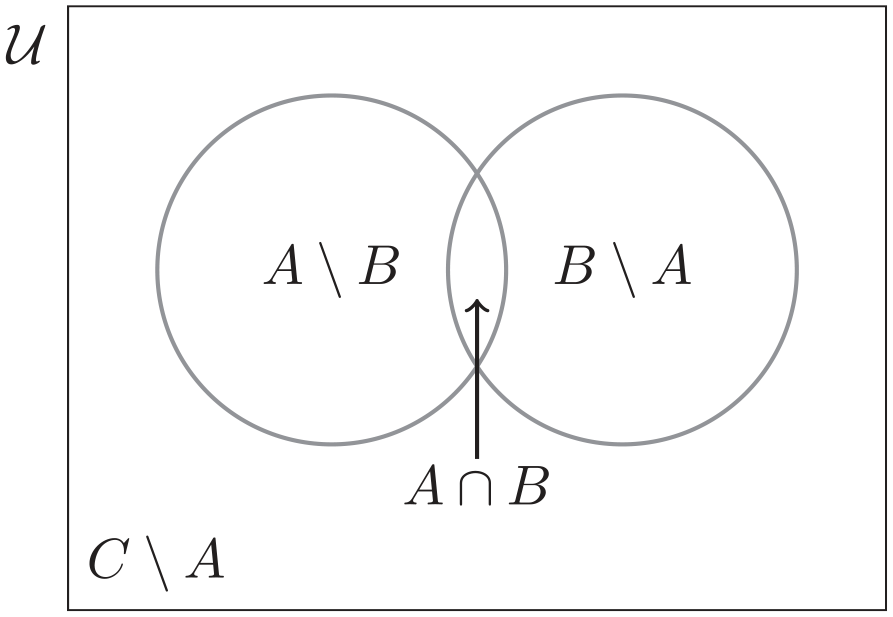
Unfortunately, non-probability data sources may suffer from quality issues. Two types of error pervading these data are coverage error (also known as selection bias) and measurement error. Coverage error occurs when we do not have a one-to-one correspondence between the population of interest and the population sampled. It may include: undercoverage, where some units in the target population have been excluded from the sampling population (e.g., new business startups not yet included on a business register at the time of a survey); overcoverage, where the sampling population includes units that are not in the target population (e.g., inactive or closed businesses); and duplication, when some units in the sampling population can be selected more than once (e.g., when a merger leads to the same business being included twice on a survey frame).
Our focus in this paper is on undercoverage error. Meng (2018) showed that undercoverage in a non-probability sample can have a significant impact on the quality of an estimate. In fact, the error can get bigger the larger the dataset is, such that it may be preferable to use a small probability sample than a large dataset containing selection bias.
We will also refer to measurement error broadly as a misalignment between the true value of a target concept, and the value actually being captured by the sample. The measurement error may thus arise due to issues such as differences in terms of how concepts are defined, recording or instrument errors, and so on. For example, a business may report their revenue in whole dollars on a survey form which is asking for reporting to be done in thousands of dollars.
In recent years, methods have been developed to address the shortcomings of these new data sources, and in particular selection bias in the non-probability sample. These methods enable the statistician to make direct use of the non-probability data to produce statistics. Generally these methods require us to have additional information from the population that we can use. The auxiliary information is typically used to correct for coverage error or to form models to impute for the missing units in the population, and could include known or estimated population totals, unit level information from a population register or frame, or from an independent probability survey sample (which we will refer to as a reference sample) taken from the same population.
In this paper, we examine and compare through a realistic and wide-ranging simulation study the effectiveness of a cross-section of the estimation methods that have been developed for non-probability data, some in combination with probability sample data. The comparison is undertaken in a business survey context. Business surveys generally have a number of characteristics that will influence the choice and performance of an estimation approach; see Hidiroglou and Lavallée (2009) for a good overview of these characteristics. For instance, there tends to be a larger quantity of auxiliary information available on a business population frame, including items that are well-correlated with the data items of interest, for example through administrative data from taxation agencies. Business data items often also have skewed distributions, while their sample designs tend to be highly stratified, with large variations in the probabilities of selection. In particular, the largest contributors tend to be included with a probability of 1. Finally, there is often a reliable identifier (such as an official business number from the tax system) available, allowing different data sources to be linked. These characteristics will influence the data available from any reference sample from a business population.
We focus on the situation where the non-probability dataset makes up a large (approximately 50%) portion of the population, an accompanying business probability sample from the population is available as auxiliary data, and the non-probability dataset can be linked to units on the probability sample and the population frame. The study explores the effects of nonignorable non-response and measurement error in the non-probability sample on the performance of the various estimators, with the probability sample used to help address these issues. To our knowledge, an empirical comparison of such a wide range of methods in a realistic business survey context has not been done before. The results from the study provide some practical insights for statistical agencies looking to use these estimators to produce inference using their own large business non-probability datasets.
The rest of the paper is structured as follows. The basic setup for this paper is outlined in Section 2. In Section 3, we provide a brief overview of the various estimation approaches that have been developed in recent years in the non-probability sample space. Section 4 discusses a number of sample design frameworks that may be used to produce reference samples to address the shortcomings of the non-probability dataset. In Section 5 we provide a description of the empirical comparison study using simulated business data and discuss the results. The simulation is grounded in data analysis of ABS Business Longitudinal Analysis Data Environment (BLADE, 2020) data and includes empirically-derived right-skewed distributions and realistic missingness scenarios in the non-probability data. We conclude with some final thoughts in Section 6.
2. Basic Setup
For each unit
Suppose we have a probability sample
Denote a non-probability dataset by
Domains within the population
Some assumptions are often made regarding the selection mechanism into
Ignorability implies that
In addition to the above, the following will be assumed in some of the methods discussed in this paper:
Assumption A4 may be satisfied if there exists a common unit identifier available on
Assumption A5 will tend not to reflect reality, especially in this age of declining response rates (Beaumont 2020). The full response assumption in
Assumption A6 implies that we have access to all auxiliary variables relevant to Assumptions A1, A2, and A3 on the datasets

where
3. Inference Methods for Non-Probability Datasets
In this section we provide a brief overview of the literature on methods developed for making inference using non-probability datasets. A number of very good review papers also exist in this space that provide more detailed discussions of the various methods. The interested reader is pointed to S. L. Lohr and Raghunathan (2017), Zhang (2019), Tam and Holmberg (2020), Yang and Kim (2020), Rao (2021), and Wu (2022). More recently, Salvatore (2023) analyzed a large number of documents on this topic using text mining and bibliometric techniques to identify current research trends.
The method of inference used depends on the data structures we have for the non-probability and reference samples. There are three general approaches that will be discussed in this paper: weighting-based approaches, imputation-based approaches, or a combination of the two (so-called doubly-robust methods).
The data available to us in
Data Structures.
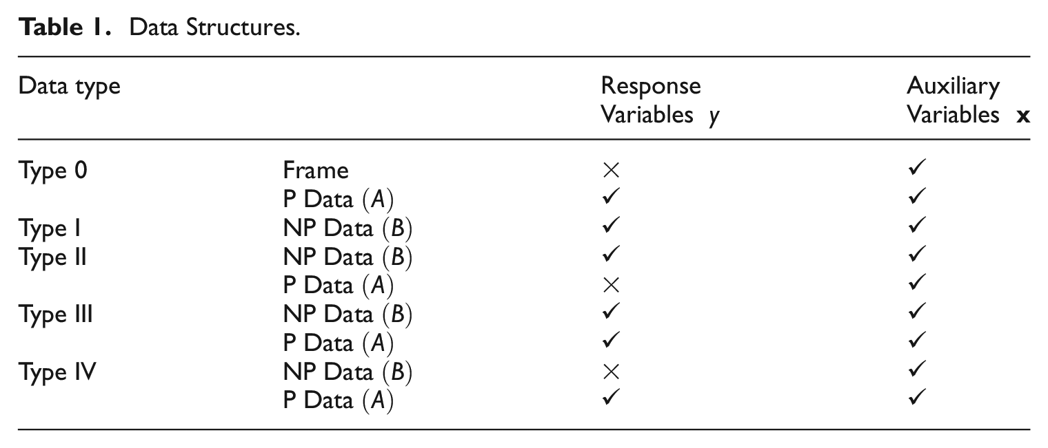
3.1. Weighting Approaches
Weighting approaches create a weight associated with each record in the reference sample or the non-probability sample, and these are used to form estimates for a target population quantity using an Inverse Probability Weighting (IPW) approach. Define
Let
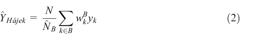
where
When a Type III data structure exists, and assuming that we can determine the value of
Rather than making a weight adjustment for the probability sample, we can instead produce a weighted non-probability sample. This seems attractive in particular when
Under Assumption A1 and a Type I data structure, selection bias may be reduced by applying a weight calibration process to

to produce final weights
Direct estimation of propensity scores
Elliott and Valliant (2017) estimate
Wang et al. (2021) proposed an Adjusted Logistic Propensity (ALP) weighting method which also pools the non-probability and probability datasets together, but does not require the assumption of non-overlapping samples. However, in their method the final estimated propensity may sometimes be greater than 1 if
If Assumption A1 does not hold and the missingness in
Machine learning techniques have also been explored to estimate the propensity scores. Ferri-García and Rueda (2020) provide a comparison of different machine learning approaches using a pooled dataset
More accurate estimated propensity scores may be achieved by incorporating known information about the auxiliary variables in the propensity score estimation for
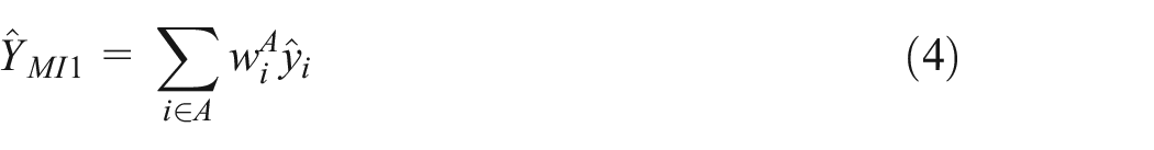
3.2. Imputation-Based Approaches
Imputation-based approaches assume that we can form a reliable estimate for
Under a Type II structure, an alternative imputation estimator to Equation (4) is (see Wu 2022)
where
Rivers (2007) proposed a sample matching approach using nearest neighbor imputation to mass impute the missing
where
When a Type IV data structure exists, the reference sample may be used to estimate the parameters of the model for
In the case where the modeling process fails to capture the true relationship between predictors and the variable of interest,
Medous et al. (2023) extended the calibration approach of Kim and Tam (2021) from a Type III to a Type IV structure, proposing so-called QR predictors (see Wright 1983) to produce an estimated
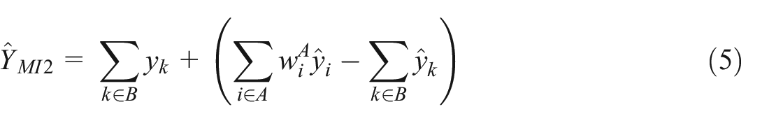
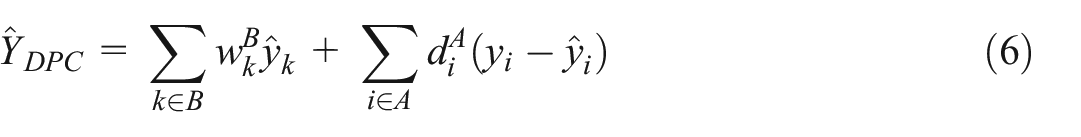
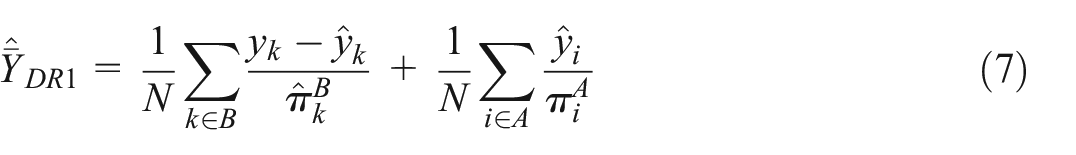
3.3. Doubly Robust Estimation
Many of the approaches outlined in the previous sections depend on an accurate working model. To protect against model misspecification, some authors have suggested doubly robust estimators constructed using both a propensity score model for
Assuming a Type II data structure, Y. Chen et al. (2020) proposed two doubly robust estimators for
and
where
The doubly robust approach can be extended to a multiply robust scenario. Instead of employing a single propensity score model to estimate
4. Alternative Sampling Frameworks for the Reference Sample
In the approaches described in Section 3, the reference probability samples
4.1. Multiple Frame Approach
The original theory for multiple-frame surveys was developed by Hartley (1962, 1974), and has been built upon in recent years; see, for example, S. Lohr and Rao (2006) and S. L. Lohr (2011). In the context of non-probability data, one can consider
Assume that we can identify

where
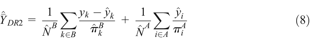
A number of assumptions are generally made when making inferences under the multiple-frame framework. Within a data integration context, some of these assumptions may be less likely to hold. One potential issue is that the variables captured on the non-probability source may not match exactly the variables of interest captured in the probability sample. If a “screening” dual frame design has been used, the lack of overlapping sample makes it more difficult to assess and address any measurement error in the non-probability dataset.
4.2. Cut-Off Sampling
In cut-off sampling, a certain fraction of the population are deliberately excluded from the survey frame. A probability sample is then taken from the remainder of the population. This practice tends to be used in business surveys when the variable of interest is highly skewed; Yorgason et al. (2011) and Elisson and Elvers (2001) provide some examples. Generally, the smallest businesses are placed into a single “take-none” stratum with zero probability of selection. The contribution of these businesses to the variable of interest is assumed to be negligible compared with the remaining part of the population, so there is a saving in terms of reduced respondent burden and cost without causing significant bias (Elisson and Elvers 2001). The rest of the population may be further divided into a “take-all” (completely enumerated) and a “take-some” (sampled) stratum. Denote the population in the take-none, take-some, and take-all strata as
The non-probability dataset would often be useful for estimating the part of the population
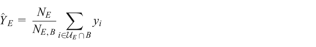
where
Note that this estimator will only be approximately unbiased if
5. Empirical Comparison of Estimation Approaches
A simulation study was conducted to compare different estimation approaches for non-probability samples within a business survey context. We selected a cross-section of approaches that would be straightforward to implement for a statistical agency. The aim of the exercise was to examine their performance under four scenarios: SAR versus SNAR missingness in the big dataset, and with versus without measurement error in
In addition to Assumptions A4 to A6 in Section 2, the simulation study assumes that the population frame includes some auxiliary information, including frame employment and industry class, and these variables are available to use during the estimation process. We can reasonably expect this to hold in a business survey context. For example, some business information is often be available from administrative sources (like business tax data) to attach to the population frame.
The simulation consisted of the following steps: (1) generating a number of data items for a finite population with distributional properties similar to some items on a real business survey dataset, (2) drawing a random subsample from the population to be the “big dataset,” (3) drawing a reference probability sample, and (4) applying some of the methods described in Section 3 to produce estimates.
For each of the sample designs considered,
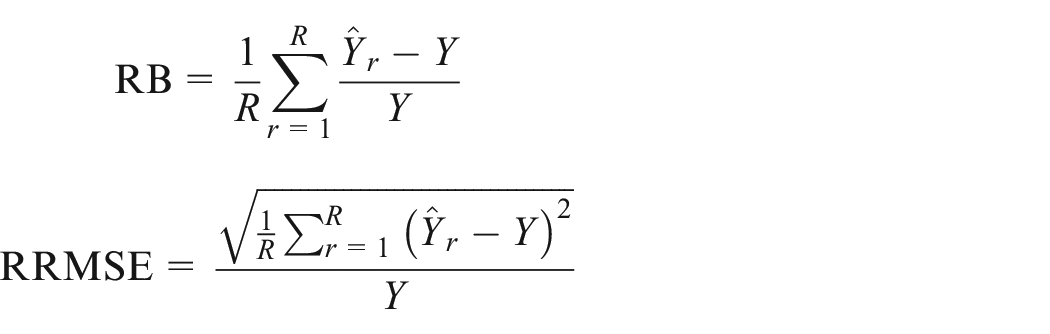
where
5.1. Generating the Population and Big Dataset
The simulated population has
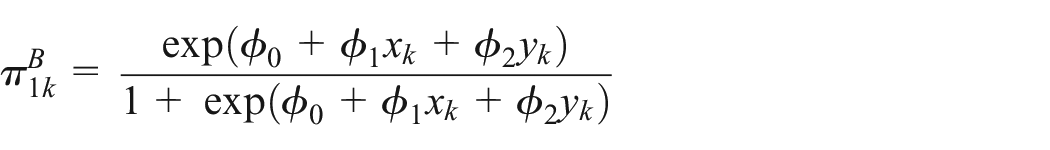
The selection mechanism for inclusion in the big dataset is given by
Two types of big dataset were produced, one following a SAR process, and one following a SNAR process.
At the second stage, the
For each sample draw of the simulation, a big dataset sample was drawn using Poisson sampling and the final
5.2. Probability Sample Designs
The population was assigned to strata based on State, Industry Division, and Frame Employment for each business. Size stratum categories were: 0 to 4 employees, 5 to 19 employees, 20 to 299, and 300+.
Three sample design scenarios were examined:
Single-frame—An optimal allocation of sample to strata using the full population frame,
Dual-frame—An optimal allocation of sample to strata using
Cut-off—An optimal allocation of sample to strata where the sampling frame is the population excluding units in the smallest (0–4 employees) size class
The Bethel-Chromy algorithm (Bethel 1989; Chromy 1987) was applied to produce optimal allocations for each of the three scenarios, treating the relevant sample frame as the population of interest. For example, in the dual-frame scenario the algorithm was applied to achieve accuracy targets based on the units in
Relative Standard Error (RSE) of 1.5% at the National level
RSE of 5% for each Industry Division
RSE of 5% for each State
A minimum sample size of 6 was applied for each sampled stratum. The 300+ size strata were designated to be completely enumerated strata with a sampling fraction of 1.
5.3. Estimators Examined
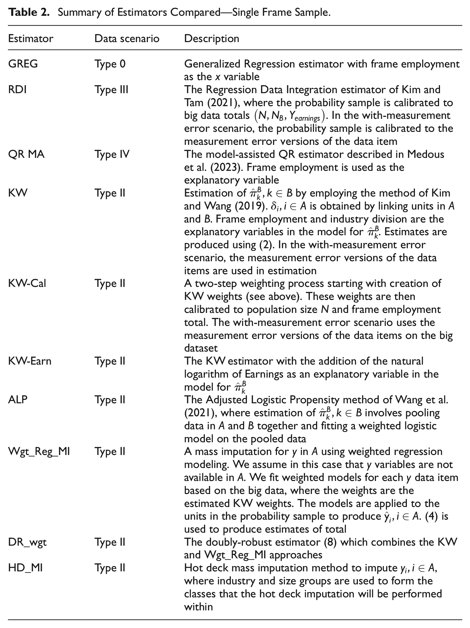
Table 2 provides a description of the estimators compared for the single-frame sample design.
Summary of Estimators Compared—Single Frame Sample.
The dual-frame probability sample design is a screening dual-frame design. This allows us to combine the estimate from the probability sample with the big data total to form an estimate for
Summary of Estimators Compared—Dual Frame Sample.
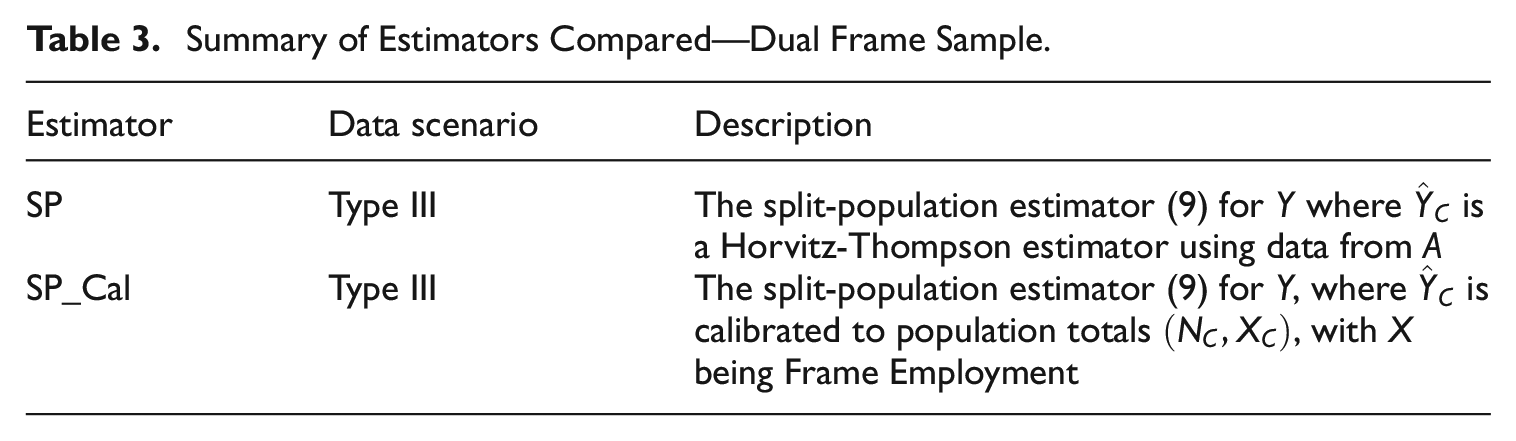
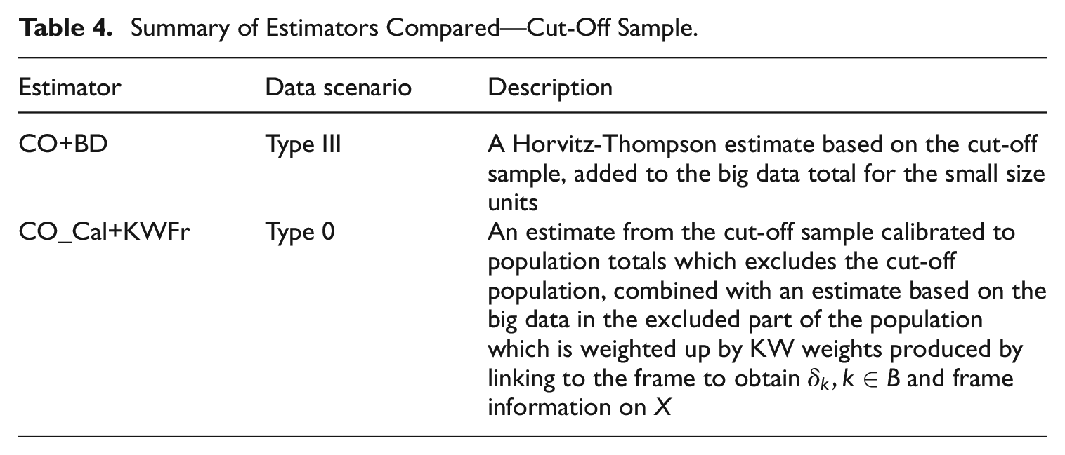
Table 4 describes the estimation methods applied to the cut-off probability sample.
Summary of Estimators Compared—Cut-Off Sample.
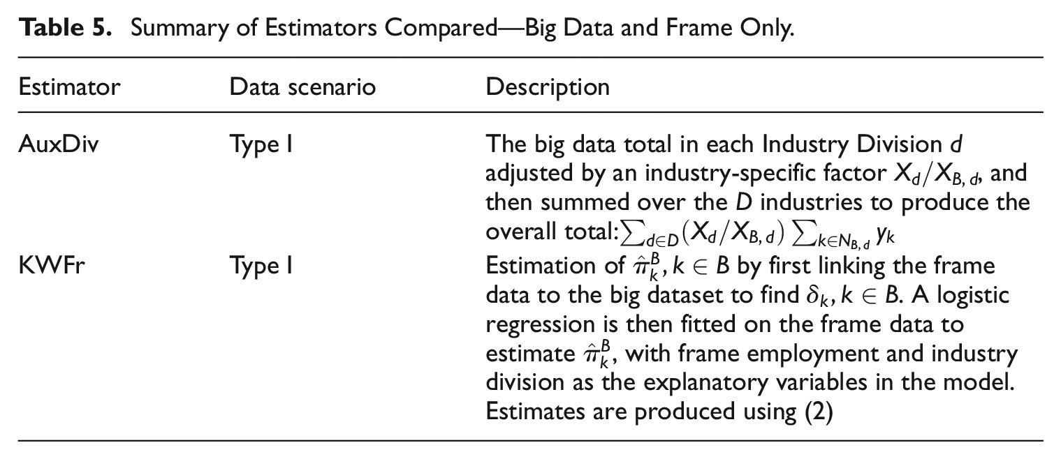
For comparison, we also produced estimates where population frame information on employment and industry were the auxiliary variables available in the estimation process. The estimators used are described in Table 5.
Summary of Estimators Compared—Big Data and Frame Only.
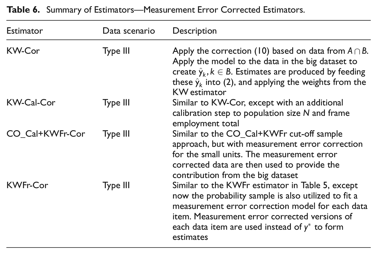
5.3.1. Measurement Error Correction in the Non-Probability Sample
By adopting the measurement error model Equation (1), we can re-arrange and obtain an expression for a measurement-error corrected version of

In a Type III data scenario, the parameters
Summary of Estimators—Measurement Error Corrected Estimators.
5.4. Results
Table 7 provides the reference sample sizes resulting from each of the different sample designs. Sample reductions are shown relative to the single-frame design. For this simulation, the dual-frame designs provide good potential for reducing the sample size, with a saving of about 40%. When using the cut-off sampling, the resulting sample savings are about 11%. Note that we did not attempt to standardize the designs in terms of the achieved precision or RMSE of estimators, as it is unclear how such a standardization would be defined when there are many variables and estimators being considered. As a result, the sample sizes achieved by the different designs need to be considered in conjunction with the RMSE results achieved by those designs in Tables 9 to 12.
Sample Sizes Under Different Designs.
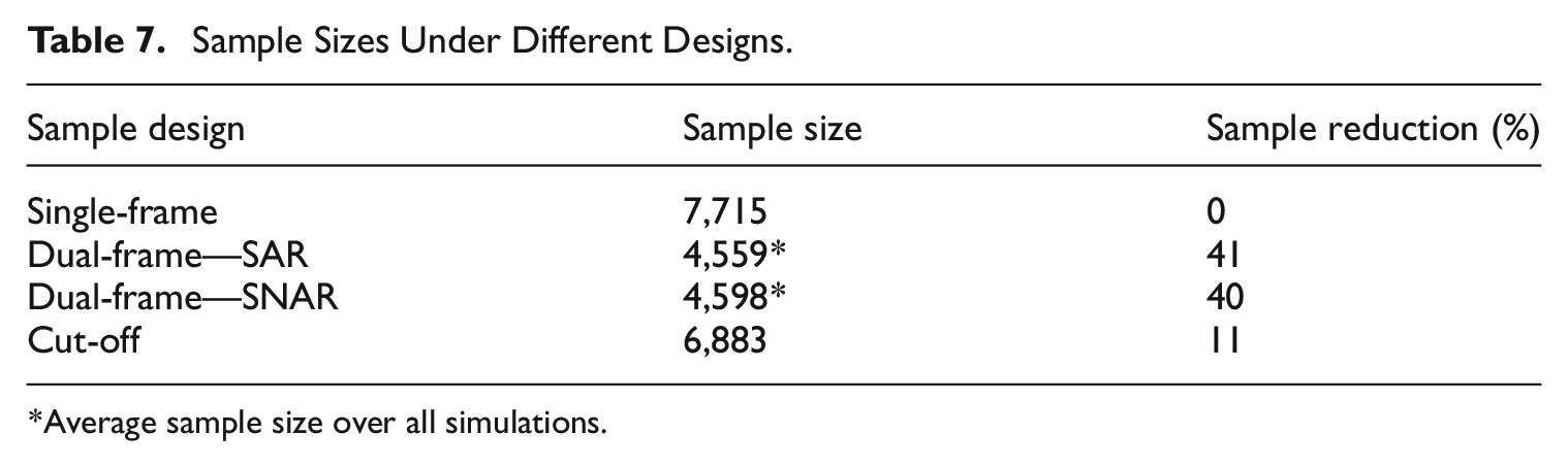
Average sample size over all simulations.
In each iteration of the simulation, national level estimates were produced for four
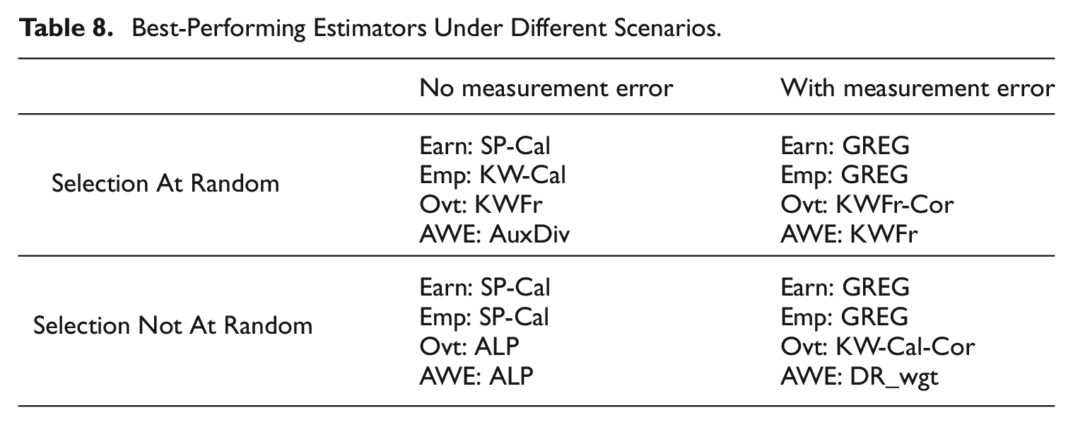
Table 8 lists the best-performing estimator in terms of RRMSE for each data item in each of the four scenarios of SAR versus SNAR and with versus without measurement error. No one estimator consistently outperforms the others in all scenarios. However, we note that the SP-Cal estimator seems to perform reasonably in the no measurement error scenario, while the GREG estimator more often performs best when there is measurement error. We next highlight our results for each of the four classes of estimators considered.
Best-Performing Estimators Under Different Scenarios.
5.4.1. Single-Frame Design Results
The GREG (Type 0 data structure), RDI (Type III), and QR MA (Type IV) estimators rely on the probability sample data for inferences, and as expected they have negligible relative bias under all missingness and measurement error scenarios we examined. These estimators are “safe” estimators, producing robust performance. Of these three estimators, the GREG with frame employment as the auxiliary variable performs best—it is also consistently among the best performers across all estimators. The RDI estimator, which relies on
When there is no measurement error, the RRMSE for the QR MA estimator is slightly higher than that for the RDI estimator, reflecting a penalty due to the fact that it estimates
A few variants of propensity score estimator were examined in our study, applicable under a Type II data structure. The KW-Cal estimator performs very well in the ideal scenario of SAR and no measurement error (see Table 9). In general, the calibration to frame employment helps to reduce the variance of the KW estimates.
Monte Carlo Bias and RRMSE of Estimators Based on 2,000 Samples—SAR, No Measurement Error.
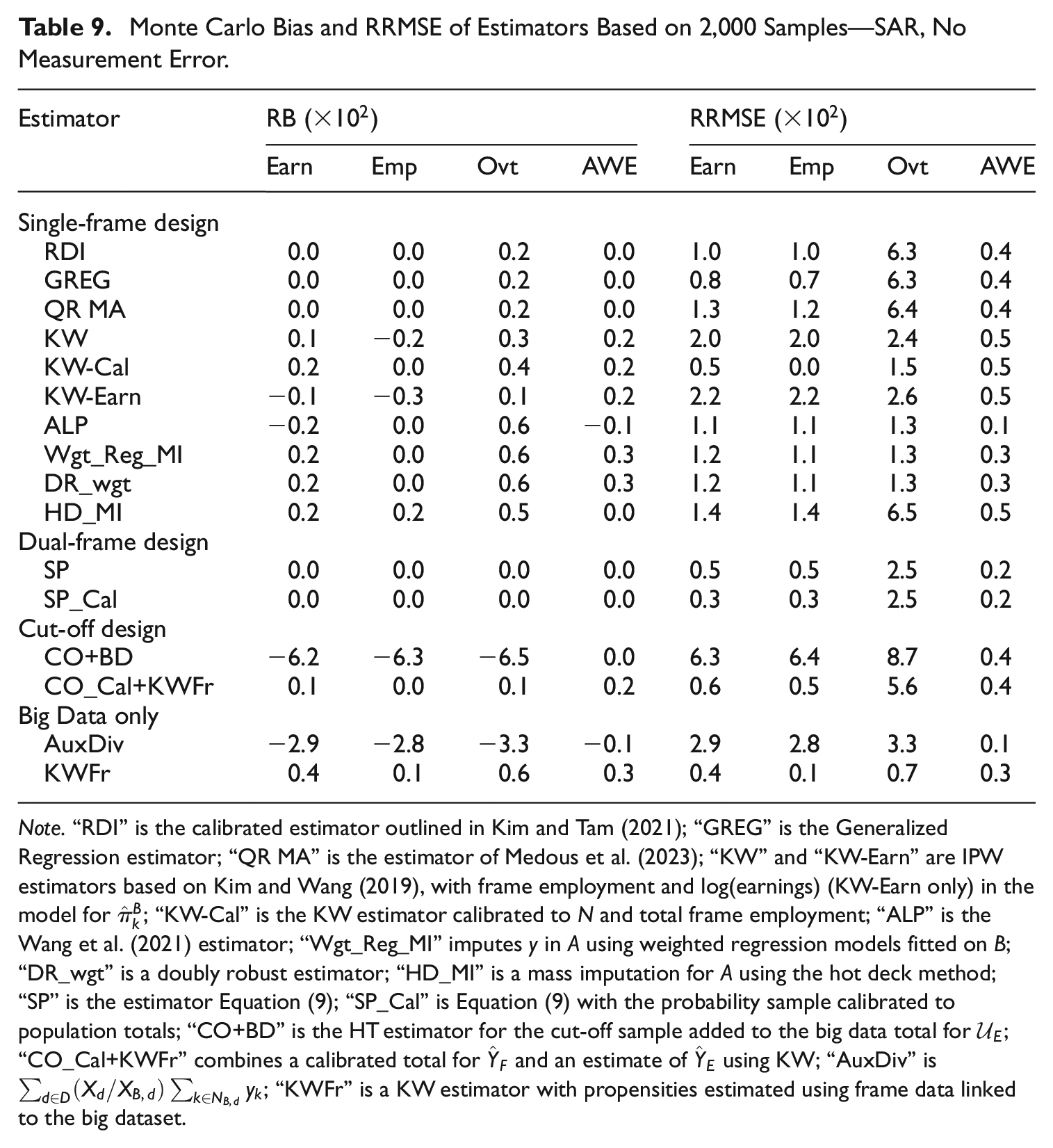
Note.“RDI” is the calibrated estimator outlined in Kim and Tam (2021); “GREG” is the Generalized Regression estimator; “QR MA” is the estimator of Medous et al. (2023); “KW” and “KW-Earn” are IPW estimators based on Kim and Wang (2019), with frame employment and log(earnings) (KW-Earn only) in the model for
The ALP estimator performs favorably as an alternative to the KW estimator, achieving a lower RRMSE in the four scenarios tested. In our simulation study, we found that some of the resulting propensities were larger than 1 when using this method, and this lead to IPW weights of less than 1. This, along with other conceptual issues with the pooled approach noted by Wu (2022), means the survey practitioner will need to consider how applicable this approach will be for their case. In our study, though, these issues did not hinder the effectiveness of the estimator to produce relatively efficient, unbiased estimates of population totals.
In the SAR case, the inclusion of earnings in the KW-Earn estimator did not produce reductions in RRMSE over the KW estimator, which is expected since in the SAR case missingness in
The performance of the mass imputation approach Wgt_Reg_MI in our study was better than the KW estimator in all scenarios, although both suffered under measurement error. The inclusion of estimated propensity weights in the regression imputation model improved the performance of the regression model, aligning with findings in Castro-Martín et al. (2022). The DR_wgt estimator, which provides protection against mis-specification in one of the IPW or Regression models, tends to have comparable RRMSE compared with the Wgt_Reg_MI estimator.
The HD_MI estimator is a non-parametric mass imputation approach for
It is worth pointing out the RRMSE results for the Overtime variable when no measurement error is present (Tables 9 and 11). The Overtime variable has a larger population variance and lower correlation with the benchmarking variable Frame Employment compared with Earnings and Reported Employment. We did not include the total value of Overtime in
More generally for Overtime when no measurement error is present, the estimators based on the probability sample
From Tables 10 and 12, the KW-based, HD_MI, Wgt_Reg_MI, and DR_wgt approaches applicable under a Type II data structure all yield poor results under measurement error due to their reliance on the data in
Monte Carlo Bias and RRMSE of Estimators Based on 2,000 Samples—SAR, with Measurement Error.
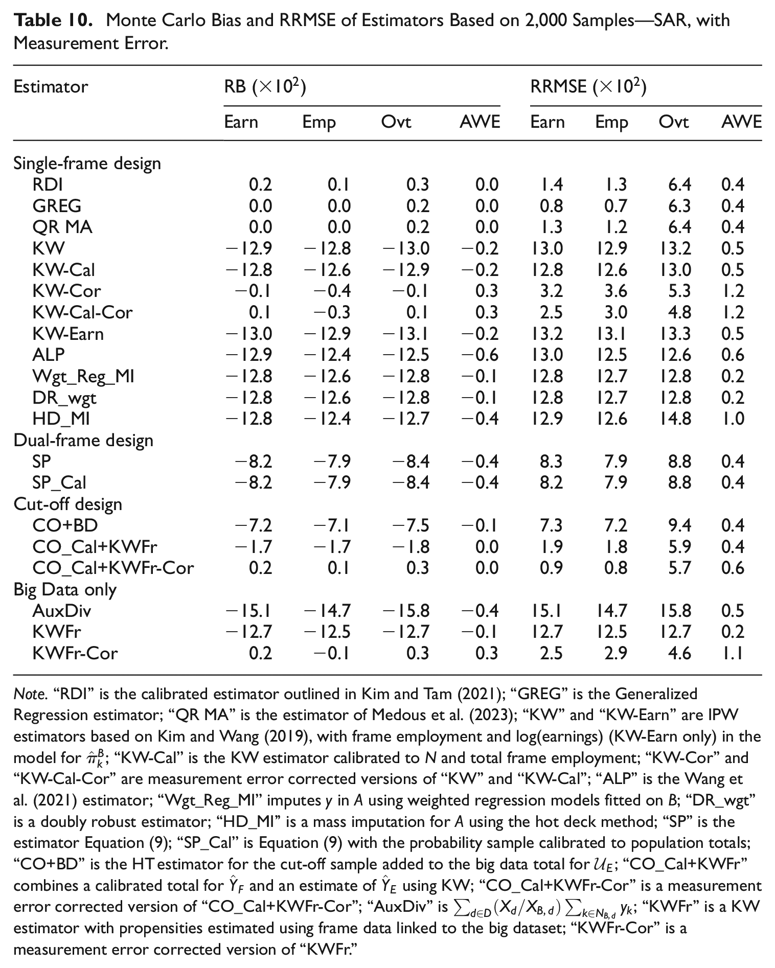
Note.“RDI” is the calibrated estimator outlined in Kim and Tam (2021); “GREG” is the Generalized Regression estimator; “QR MA” is the estimator of Medous et al. (2023); “KW” and “KW-Earn” are IPW estimators based on Kim and Wang (2019), with frame employment and log(earnings) (KW-Earn only) in the model for
5.4.2. Dual-Frame Design Results
In the without measurement error scenarios, the split-population estimators are unbiased, and their RRMSE results are generally among the lowest of all estimators we examined across SAR and SNAR settings (see Tables 9 and 11). Including a calibration to auxiliary population totals for the dual-frame estimator helps to reduce RRMSE even further for earnings and reported employment.
Monte Carlo Bias and RRMSE of Estimators Based on 2,000 Samples—SNAR, No Measurement Error.
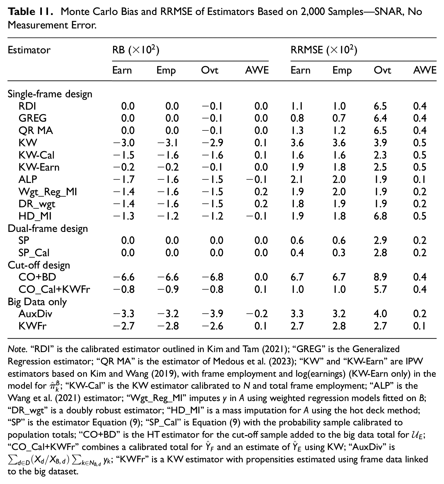
Note.“RDI” is the calibrated estimator outlined in Kim and Tam (2021); “GREG” is the Generalized Regression estimator; “QR MA” is the estimator of Medous et al. (2023); “KW” and “KW-Earn” are IPW estimators based on Kim and Wang (2019), with frame employment and log(earnings) (KW-Earn only) in the model for
However, measurement error in
Monte Carlo Bias and RRMSE of Estimators Based on 2,000 Samples—SNAR, with Measurement Error.
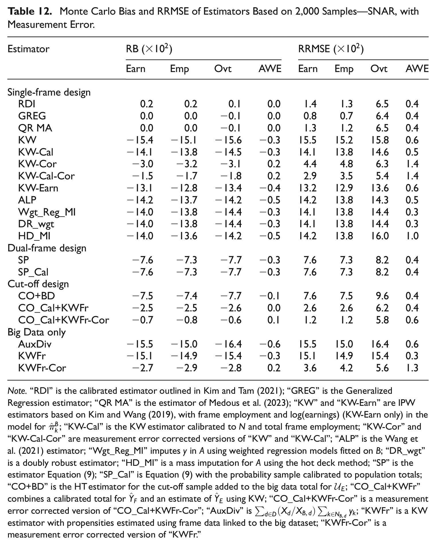
Note.“RDI” is the calibrated estimator outlined in Kim and Tam (2021); “GREG” is the Generalized Regression estimator; “QR MA” is the estimator of Medous et al. (2023); “KW” and “KW-Earn” are IPW estimators based on Kim and Wang (2019), with frame employment and log(earnings) (KW-Earn only) in the model for
5.4.3. Cut-Off Design Results
The results for the estimators using the cut-off sample design show that in our case simply combining the reference sample and the portion of
The CO_Cal+KWFr estimator aims to account explicitly for the contribution of the excluded part of the population
In the SAR without measurement error scenario (Table 9) there is little reason to opt for the CO_Cal+KWFr estimator rather than the KWFr estimator. In this case, where the quality of the data in
For the worst-case SNAR with measurement error scenario, the CO_Cal+KWFr-Cor estimator yielded close to the lowest overall RRMSE for the data items of interest (see Table 12). This was the case even though the contribution from the KW estimator did not fully reflect the non-response mechanism since that estimator did not include earnings (hence there is still a negative bias in the estimates obtained). This demonstrates the benefit of not relying solely on
5.4.4. Big Data Only Results
When aggregate auxiliary information is available from the population it can be used to help reduce selection bias, as evidenced by the performance of the AuxDiv estimator. The AuxDiv estimator does not remove all bias as it does not include all of the
The KWFr estimator performs very well in the SAR without measurement error scenario (see Table 9), achieving close to the lowest RRMSE for all data items. This estimator uses unit-level auxiliary information for the full population to estimate the propensity scores for the large dataset
Measurement error degrades the performance of the KWFr estimator (see Tables 10 and 12). Similarly, in the SNAR scenarios the estimator does not perform as well since it is not able to include the earnings variable in the propensity model. The results for the KWFr and AuxDiv estimators demonstrate that relying on the non-probability dataset itself for inference are likely to lead to biased estimates if there are inherent issues with either the measurement of its data items or incompleteness of available auxiliary information from the population frame.
6. Concluding Remarks
A variety of approaches, ranging from weighting-based methods, to model-based or imputation approaches, to combinations of the two, have been developed to address the faults of non-probability data. The objective of this paper is to compare how a range of these methods perform in business survey context assuming different missingness and measurement error settings for a large non-probability dataset, and a reference probability sample available to assist. The results in the paper provide valuable insight into the usefulness of these methods under various conditions, and are important for increasing the efficiency of statistics produced while reducing respondent burden and sample sizes.
When auxiliary information, related to
When there is SNAR missingness in the non-probability dataset but no measurement error, the calibrated split population estimator still provides the best results. This approach is robust to the selection mechanism at play in the non-probability dataset, since we use the non-probability data as-is and supplement it with data from the reference sample to cover the contribution for the population not in the non-probability dataset. The estimator is more efficient for large non-probability datasets. In situations when the non-probability dataset is a small fraction of the population, for example a small web panel survey, the performance of the estimator will be closer to the GREG.
The presence of measurement error in the non-probability data source affects the performance of the estimators, such that the best estimator tended not to heavily rely on the non-probability data. In our study, the GREG, RDI, and QR MA estimators—all of which rely on the reference sample as the basis for estimation—tended to perform the best in the with measurement error scenarios. An advantage of the RDI estimator over the measurement error corrected estimators listed in Table 6 is that we can continue to use the
The corrected cut-off estimator, which combines the cut-off sample contribution with an estimate for the excluded part of the population, also performs well under measurement error. Further research could be beneficial for determining appropriate cut-off thresholds for the reference sample which take advantage of the ability to model or estimate the contribution from the excluded part of the population based on the available non-probability data.
Collecting information on the data item(s) of interest in the probability sample would assist with developing a model to correct for measurement error. One factor to be wary of is that the measurement error model may introduce additional variability into the estimates, so that we may choose instead to use the probability sample as the basis for inference and not rely on the non-probability data.
Although the RDI estimator is never the best-performing estimator, it is (asymptotically) unbiased, and has a reasonably low RRMSE in all scenarios. The estimator is also robust to SNAR situations as well as the presence of measurement error, but its efficiency can suffer under those less-than-ideal scenarios. When data for
Many of the methods that have been developed make two assumptions: ignorability, which implies a SAR scenario in the non-probability data source, and common support, which implies that the probability of being in the non-probability dataset
Including all
Supplemental Material
sj-docx-1-jof-10.1177_0282423X241298243 – Supplemental material for An Empirical Comparison of Methods to Produce Business Statistics Using Non-Probability Data
Supplemental material, sj-docx-1-jof-10.1177_0282423X241298243 for An Empirical Comparison of Methods to Produce Business Statistics Using Non-Probability Data by Lyndon Ang, Robert Clark, Bronwyn Loong and Anders Holmberg in Journal of Official Statistics
Footnotes
Acknowledgements
The authors are grateful to three anonymous referees and an associate editor for their constructive comments, which have improved this article greatly. The authors would like to thank Dr. Siu-Ming Tam and Dr. Ryan Covey for their constructive comments on an early draft of this manuscript. The first author benefited from email exchanges with the authors of some of the methods investigated in this paper, including Prof. Yan Li and Prof. Pengfei Li.
Funding
The author(s) disclosed receipt of the following financial support for the research, authorship, and/or publication of this article: The first author was supported by funding from the Sir Roland Wilson Foundation and the Australian Bureau of Statistics.
Disclaimer
The views expressed in this paper are those of the authors and do not necessarily represent the views of the Australian Bureau of Statistics. Where quoted or used, they should be attributed clearly to the authors.
Supplemental Material
Supplemental material for this article is available online.
Received: May 2024
Accepted: October 2024
References
Supplementary Material
Please find the following supplemental material available below.
For Open Access articles published under a Creative Commons License, all supplemental material carries the same license as the article it is associated with.
For non-Open Access articles published, all supplemental material carries a non-exclusive license, and permission requests for re-use of supplemental material or any part of supplemental material shall be sent directly to the copyright owner as specified in the copyright notice associated with the article.