Turnover Flash Estimation by Purposive Sampling and Debit Card Transactions

Abstract

Improving timeliness is ever more urgent for official statistics, not least due to the potentials of various non-survey big data that in principle can be made more quickly available than traditional sample surveys. Taking Retail Turnover Index as the case-in-point, we develop new approaches of model learning aimed to achieve flash estimation of acceptable accuracy, as well as the associated methods of uncertainty assessment, when one does not have the target observations that would have been required for unbiased inference by established statistical theories. Applications to the Norwegian data will be used to demonstrate the efficacy of our proposals.

1. Introduction

Using non-survey big data to produce rapid estimates of economic indicators has attracted attention in recent years. See Baldacci et al. (2016) and Eurostat (2017) for two early overviews on the relevant background, methods, and challenges, from the perspective of official statistics and under the auspices of Eurostat and United Nations.

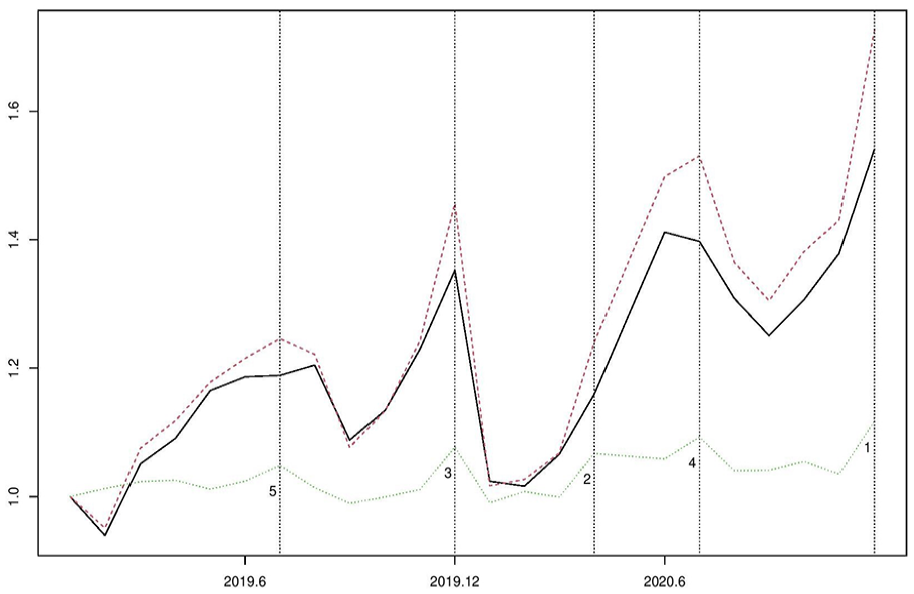
Figure 1 shows the Norwegian Retail Turnover Index (RTI) in the years 2019 and 2020, together with an index calculated from retail transactions directly. This “transaction index” was made available due to the emergency of the covid pandemic in 2020. It is based on the payment total of all domestic debit cards and one major internet payment platform. The ratio ${\tilde{I}}_{t-1,t}/I_{t-1,t}$ between the month-on-month transaction index ${\tilde{I}}_{t-1,t}$ and RTI $I_{t-1,t}$ , where $t$ denotes month, is given in Figure 1 and the five largest fluctuations are marked. Although the two indexes are well correlated, the ratio between them fluctuates too much for the transaction index to be accepted as official statistics, given its obvious error sources pertaining to coverage, measurement, business unit delineation, and population domain classification. For instance, by definition retail trade turnover comprises the total invoiced by the statistical unit during the reference period. It includes all charges such as packaging and transport but excludes VAT and similar deductible taxes; but the deductible taxes cannot be separated from the debit card payment transaction totals.

Figure 1.

Retail Turnover Index (solid line) and a transaction index (dashed line) in Norway over twenty-four months in 2019 and 2020. Five largest fluctuations of month-on-month index ratio between them (dotted line) marked by vertical lines (1, …, 5).

This exemplifies a situation where some survey data may still be necessary for producing official statistics, in addition to relevant and timely big data. However, to shorten the lag between dissemination time point and statistical period, one may be prepared to “give up waiting” on the sample units that have not yet responded, if the available non-survey big data can compensate for the loss of information, thereby making flash estimation or nowcasting possible. For instance, Fornaro and Luomaranta (2020) combine traffic volume records with early available firm data for nowcasting Finnish quarterly Gross Domestic Product and Trend Indicator of Output.

For our focus in this paper, the Norwegian RTI for NACE45-47 is currently published by the 30th day after the calendar month $t$ , denoted by $t+30$ . NACE is the statistical classification of economic activities in the European Community and is the subject of legislation at the European Union level. By NACE45-47, we refer to G45—Wholesale and retail trade and repair of motor vehicles and motorcycles, G46—Wholesale trade, except of motor vehicles and motorcycles, and G47—Retail trade, except of motor vehicles and motorcycles. For each month $t$ , the survey sample has two parts, where $s_t$ denotes the self-representing (or take-all) units with inclusion probability one, and $r_t$ denotes the rest take-some units with inclusion probability less than one. The units in $s_t$ are larger on average; more importantly, they mostly belong to business chains, for which the turnover values can be obtained quickly from the chain headquarters, whereas it takes longer for many units in $r_t$ to respond.

Thus, in order to achieve flash estimation at an earlier time point, as well as to reduce response burden and processing cost, we propose to investigate model-based estimation given only the take-all sample in NACE47 and with the help of all available transactions and administrative data. If feasible, then no sample units will be needed from outside the take-all units, which amounts to adopting a purposive sampling design.

Note that we approach flash estimation as a problem of prediction for the unobserved or out-of-sample units. This allows one to make use of past survey and non-survey data at the business unit level in a flexible manner, and enables novel statistical learning approaches. Since the unit-level prediction errors can be gauged retrospectively, for example, by comparisons to the VAT turnover values, the approach provides also means to detect outliers and other anomalies, which can be helpful for the maintaining and updating the purposive sample that still needs to be surveyed directly.

Note also that the focus on NACE47 at this stage has two reasons. First, the RTI used to be limited to NACE47 before its scope was extended in 2021, and many users actually are still interested in the RTI for NACE47. Second, Statistics Norway currently have only access to debit card transactions data, which have the highest share among all payment transactions in NACE47, while the other forms of payment have a greater share in NACE45-46. Confidentiality of personal data is protected as the transactions are aggregated for each business unit by the debit card payment service operators, and only the totals for each business unit are delivered to Statistics Norway.

In short, we shall consider the strategy of model-based flash RTI using purposive sampling and debit card transactions for NACE47. Provided the turnover values can be obtained from most of the take-all units by $t+7$ , it is envisaged that the Retail Volume Index for NACE47 can be produced by $t+15$ , allowing for the necessary post-RTI processing. This will halve the thirty-day lag of dissemination that is common internationally, while at the same time reducing survey response burden and processing cost.

However, the feasibility of this strategy depends on whether (model) learning can be organized in a fruitful way in the case of purposive sampling, which means that no target observations (of turnover) are at all available for the non-take-all units at the time of flash estimation.

We shall formulate and investigate two new learning approaches. First, by adapting a loss function that bears some semblance to regularization, such as LASSO (Tibshirani 1996), we devise augmented learning that allows one to learn from both the past non-take-all units and current take-all units. Next, taking inspirations from the field of transfer learning (e.g., Ng 2016; Pratt 1993), we formulate quasi transfer learning for situations where observations of the target model can only become available retrospectively.

Although in concept neither form of learning can yield unbiased prediction for the unobserved units, they may be able to reduce the errors of learning only from the purposive sample (which is also biased generally). Moreover, in addition to explaining how the chosen model and learning approach can be validated retrospectively based on relevant VAT data from tax administration, we shall develop a novel approach to real-time error prediction for the flash RTI. In particular, two key points of this error prediction approach applies generally to flash estimation: (a) error prediction is a distinct learning task to outcome prediction because, in the absence of relevant target observations, one cannot pretend that the adopted model would yield unbiased prediction of the target outcome (such as turnover here) and derive the associated uncertainty as a by-product of the outcome model, (b) to improve the efficiency of error prediction one should utilize observed unit-level prediction errors in the past just like one would use observed past outcomes for outcome prediction.

The ideas above will be developed in Section 2 and applied in Section 3 to the Norwegian data in years 2019 to 2022. Some final remarks on implementation and future research topics will be given in Section 4.

2. Methods

We shall consider the following generic setup for flash estimation. Denote by $y$ the target outcome and $x$ the associated features. Denote by $\mu (x,s)$ a predictor for any unit with features $x$ , which is learned from $\{(y_i,x_i):i\in s\}$ , where $s$ is the training sample of observations. Denote by $R$ a target set of units with known $x_j$ , $\forall j\in R$ and $s\cap R=\varnothing$ , for which the predicted $y$ -values are of interest. However, it is known that $\mu (x,s)$ is biased for $\{y_j:j\in R\}$ , because $y_j$ for $j\in R$ and $y_i$ for $i\in s$ do not have the same distribution conditional on $x_j$ and $x_i$ .

In terms of the Norwegian RTI, $y$ is the retail turnover value excluding VAT, whereas one may include in $x$ turnover values according to the VAT register and debit card payment totals. The transactions data improve the timeliness of feature since VAT turnover values are only available with a delay of several months, whilst the payment transaction totals are available for the month $t$ before t + 7. (More details of these features will be given in Section 2.2.) Notice that for a unit that has both observed VAT turnover and transaction total, its survey turnover value often differs to its VAT turnover value reported to the tax authority, and both these turnovers will surely differ to the payment transaction total that includes VAT or other surcharges.

As a simplistic approach of learning for flash estimation, one may obtain $\mu (x,s_t)$ only based on the take-all units that are available by $t+7$ , which yields ${\hat{y}}_j=\mu (x_j,s_t)$ for any $j\notin s_t$ . The approach is called simplistic not only because $\mu (x,s_t)$ is known to be biased for the units outside $s_t$ but also because it provides naturally a baseline of comparison. Below we consider two learning approaches that aim to reduce the bias of the simplistic approach.

2.1. Augmented Learning

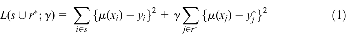
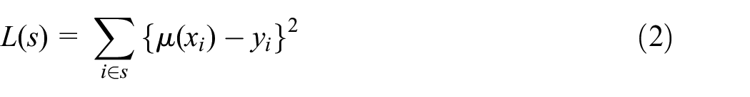
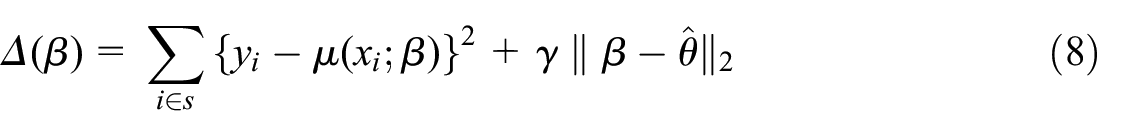
Given a constant $\gamma >0$ , let the augmented loss function be

$$L(s\cup r^{\ast };\gamma )=\sum _{i\in s}{\{\mu (x_i)-y_i\}}^2+\gamma \sum _{j\in r^{\ast }}{\{\mu (x_j)-y_j^{\ast }\}}^2$$

(1)

where $r^{*}$ denotes a set of units that are similar to or even overlap with those in $R$ , but $y_j^{*}$ is a proxy to the target observation $y_j$ including when $j\in r^{*}\cap R$ . The values $\{(x_j,y_j^{*}):j\in r^{*}\}$ may either be contemporaneous with $\{(x_i,y_i):i\in s\}$ or from some earlier time points. For predicting $\{y_j:j\in R\}$ , where $s\cap R=\varnothing$ , we would like to investigate whether $\mu (x)$ obtained from minimizing $L(s\cup r^{*};\gamma )$ may improve simplistic learning that minimizes the loss function

$$L(s)=\sum _{i\in s}{\{\mu (x_i)-y_i\}}^2$$

(2)

Note that the augmented loss Equation (1) is not a form of regularization (e.g., Hastie et al. 2009), because the second term involving $\gamma$ is not a penalty introduced to reduce the variance of unconstrained learning from $s$ , such as when the size of $s$ is small compared to the number of unknowns in $\mu (x)$ . Rather, augmenting $s$ by $r^{*}$ in (1) primarily aims to reduce the bias of learning only from $s$ , by incorporating the additional observations $\{(x_j,y_j^{*}):j\in r^{*}\}$ that may resemble the unobserved $\{(x_j,y_j):j\in R\}$ for the purpose of model learning.

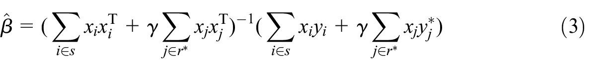
Now, in the case of linear predictor $\mu (x)=x^{\mathrm{T}}\beta$ , the estimator $\hat{\beta }$ minimizing Equation (1) is given by

$$\widehat{\beta }={(\sum _{i\in s}{x}_i{x}_i^{\mathrm{T}}+\gamma \sum _{j\in r^{\ast }}{x}_j{x}_j^{\mathrm{T}})}^{-1}(\sum _{i\in s}{x}_i{y}_i+\gamma \sum _{j\in r^{\ast }}{x}_j{y}_j^{\ast })$$

(3)

This is the same as minimizing Equation (2) based on an augmented sample

$$s^{\ast }=r^{\ast }\cup s\cup \dots \cup s$$

instead of $s$ , where $s$ is duplicated ${\gamma }^{-1}$ times in $s^{*}$ (if practically possible).

The equivalence between working with the augmented loss $L(s\cup r^{*};\gamma )$ and the simple loss $L(s^{*})$ based on an augmented sample can be exploited practically. For an arbitrary model or algorithm $\mu$ , one can obtain $\mu (x,s^{*})$ by training on an augmented sample $s^{*}$ using standard softwares, instead of working with $L(s\cup r^{*};\gamma )$ which may require weighting the observations or other adjustments that are not necessarily implemented by the available software. Instead of choosing a value for $\gamma$ , one can directly experiment with how to mix $s$ with other units that may be relevant. We refer to this as augmented learning, that is, minimize $L(s^{*})$ given by Equation (2) based on

$$s^{\ast }=s\cup r^{\ast },\{(x_i,y_i):i\in s\},\{(x_j,y_j^{\ast }):j\in r^{\ast }\}.$$

(4)

2.2. Turnover Flash Estimation by Augmented Learning

To obtain a turnover flash estimator for each month $t$ , consider augmented learning that is targeted at the units in $R_t=U_t\backslash s_t$ immediately after $\{y_i:i\in s_t\}$ become available, where $U_t$ denotes the target population for month $t$ (whether or not it is actually held fixed over any given period in practice).

Let $y_{\mathrm{ti}}$ be the turnover of business unit $i$ in month $t$ . Let the associated feature vector $x_{\mathrm{ti}}$ be selected from the VAT turnovers and debit card payment totals. The VAT register is updated every two months in Norway. At a given month $t$ , the six most recent VAT turnover values would cover a twelve-month period, which dates backwards from three or four months before $t$ . The debit card payment total is available on a daily basis, including the month $t$ of interest.

Next, for each month $t$ , let the augmented sample be given as

$$s_t^{\ast }=s_t\cup r_t^{\ast }$$

(5)

There are two settings for $r_t^{*}$ . In setting-I, where take-some units are sampled but $r_t$ is not ready for month- $t$ flash estimation, we may for example, consider

$$r_t^{\ast }=r_{t^{\prime }},r_t^{\ast }=r_{t-1}\mathrm{or}{r}_t^{\ast }=r_{t^{\prime }}\cup r_{t-1}$$

(6)

where $r_{t\prime }$ denotes the $r$ -sample (of take-some units) for the same month in the previous year, and $r_{t-1}$ denotes the $r$ -sample for the previous month. The value $y_j^{*}$ for $j\in r_t^{*}$ is a past survey turnover value, which is available by month $t$ even in case it was unavailable for month- $(t-1)$ flash estimation.

In setting-II, where non-take-all units are not sampled at all, we may for example, consider

$$r_t^{\ast }=R_{t^{\prime }}^{\ast },r_t^{\ast }=R_{t-d}^{\ast }\mathrm{or}{r}_t^{\ast }=R_{t^{\prime }}^{\ast }\cup R_{t-d}^{\ast }$$

(7)

where $R_{t\prime }^{*}$ contains all the non-take-all units with VAT turnover values for the same month in the previous year, and $R_{t-d}^{*}$ denotes this rest population for month $t-d$ . We can choose $d=4$ in Norway to ensure that the associated VAT turnover values $y_j^{*}$ have become available for any $j\in r_t^{*}$ .

Notice that in either setting, there will be many units in $r_t^{*}$ selected from the past that still belong to the population at time $t$ . While we do not observe $y_{\mathrm{ti}}$ for such a unit at the time, we may have either its past survey turnovers in setting-I or VAT turnovers in setting-II. The idea of augmented learning is to incorporate these observations to train the model for prediction at time $t$ , which can be helpful if $y_{\mathrm{ti}}$ relates to $x_{\mathrm{ti}}$ in a similar manner as $y_{t^{*}i}^{*}$ relates to $x_{t^{*}i}$ given sensible choice $t^{*}$ or composition of $r_t^{*}$ ,

2.3. Quasi Transfer Learning

Denote by $\mu (x;\beta )$ a target model with unknown parameters $\beta$ . Suppose there exists a relevant source model for a different though similar population, which has been estimated separately, denoted by $\mu (x;\hat{\theta })$ , where the two models belong to the same family with different parameter values $\beta$ and $\theta$ . Transfer learning in such a setting aims to improve the estimation of $\beta$ by leveraging $\hat{\theta }$ .

For instance, one may estimate $\beta$ based on the target observations that are associated with the units in $s$ , subject to a chosen penalty of the discrepancy between $\beta$ and $\hat{\theta }$ , such as minimizing

$$\Delta (\beta )=\sum _{i\in s}{\{y_i-\mu (x_i;\beta )\}}^2+\gamma \parallel \beta -\widehat{\theta }{\parallel }_2$$

(8)

given $\gamma >0$ . Although the resulting estimator of $\beta$ is biased generally due to the penalty term, the variance of estimation is reduced compared to estimating $\beta$ only based on $s$ . One can thus view the approach as a form of regularization, which has shown to be especially helpful in cases with insufficient number of target observations (e.g., Gu et al. 2023; Li et al. 2020).

However, there is an essential difference to our setting for flash estimation outlined at the beginning of Section 2, in that we have no target observations at all from $R$ and the model trained on $s$ is biased for predicting the units in $R$ . We therefore formulate an approach that will be referred to as quasi transfer learning. Let the learning for RTI flash estimation target the model for

$$q_t=s_t\cup r_t\mathrm{or}{q}_t=s_t\cup R_t$$

(9)

which is partially covered by the available $s_t$ although by stipulation $s_t$ is not “representative” of $q_t$ . Let the choice of $r_t$ or $R_t$ in $q_t$ vary if the take-some sample $r_t$ is only unavailable for flash estimation or abolished altogether. The term “quasi” indicates that we are aiming at something that is not the target model of interest directly but close to it.

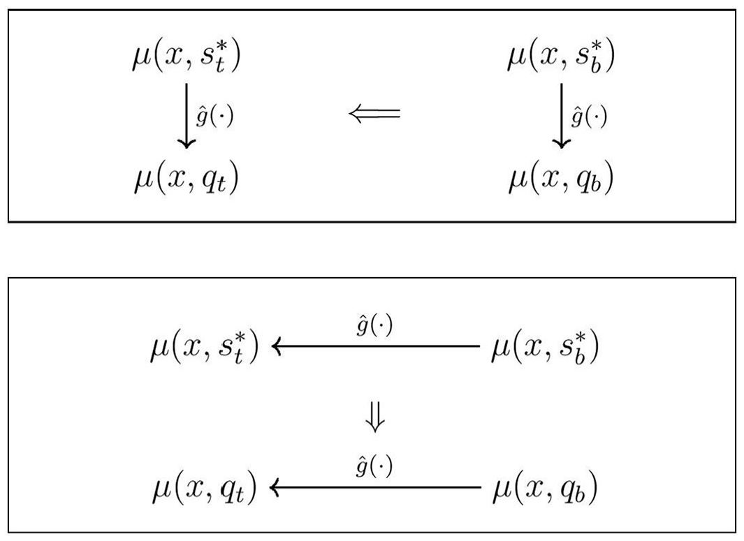
Let a relevant source model be fitted to $s_t^{*}$ , as given by Equation (5), denoted by $\mu (x,s_t^{*})$ . To leverage it for $\mu (x,q_t)$ , choose additionally two source models $\mu (x,s_b^{*})$ and $\mu (x,q_b)$ in the same setup as $\mu (x,s_t^{*})$ and $\mu (x,q_t)$ but for some time point $b$ in the past, and a transfer scheme such as the two illustrated in Figure 2.

Figure 2.

Two schemes of quasi transfer learning.

In scheme A, the estimated relationship $g(·)$ between $\mu (x,s_b^{*})$ and $\mu (x,q_b)$ at the past time point $b$ is transferred to the current time point $t$ . For instance, one can introduce a model where $\mu (x,s_b^{*})$ either figures simply as an offset or is used as a feature generally, that is,

$$E\{\mu (x,q_b)\}=\mu (x,s_b^{\ast })+g(x)$$

(10a)

$$E\{\mu (x,q_b)\}=g(x,\mu (x,s_b^{\ast }))$$

(10b)

In scheme B, the estimated relationship $g(·)$ between $\mu (x,s_t^{*})$ and $\mu (x,s_b^{*})$ over the time points $(t,b)$ is transferred to that between $\mu (x,q_t)$ and $\mu (x,q_b)$ over the same $(t,b)$ . One can introduce two models similarly to (10a) and (10b), that is,

$$E\{\mu (x,s_t^{\ast })\}=\mu (x,s_b^{\ast })+g(x)$$

(11a)

$$E\{\mu (x,s_t^{\ast })\}=g(x,\mu (x,s_b^{\ast }))$$

(11b)

The scheme A requires the relationship between $s_t^{*}$ and $q_t$ to be stable over time. This may be possible for populations that evolve slowly over time, but it is likely to be unrealistic for short-term Turnover Statistics. The scheme B requires the relationship between $s_t^{*}$ and $s_b^{*}$ over the chosen time lag to be similar to that between $q_t$ and $q_b$ over the same time lag, where $s_t^{*}$ and $s_b^{*}$ have the same sample composition and likewise for $q_t$ and $q_b$ . Moreover, at any given time point $t$ , $s_t^{*}$ and $q_t$ overlap each other in terms of $s_t$ , while the units $s_t^{*}\backslash s_t$ and $q_t\backslash s_t$ are comparable and possibly overlapping as well.

2.4. Retrospective Validation

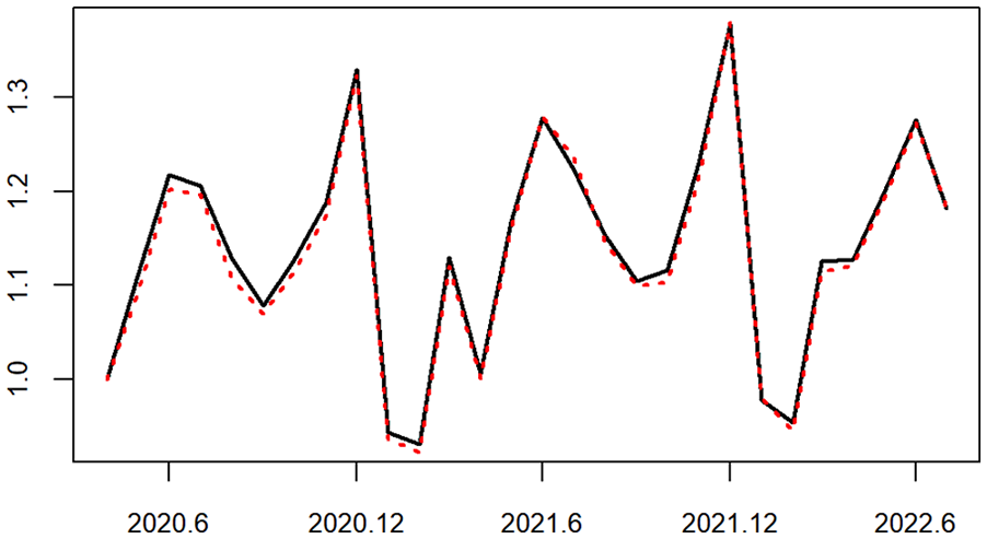
As shown in Figure 3, the survey-based Norwegian RTI tends to agree closely with the “VAT index” calculated from the VAT turnover values, although the two turnover values often disagree with each other at the unit level.

Figure 3.

RTI (solid line) and VAT index (dotted line) in Norway over 2020 to 2022.

The VAT register data can therefore provide trustworthy means of validation retrospectively. In particular, one should be able to tell if the chosen model and learning approach for flash estimation have worked satisfactorily, till as recently as $d$ months ago, had VAT turnover been the target measure. Such an approach of retrospective validation is described below.

To fix the idea, let $\mu (x)$ be the adopted working model (say, linear regression) with selected features, and let ${\mu }_t(x)$ be the predictor applied to the units in $R_t$ , which is obtained by the chosen learning approach (say, augmented learning). For validation purposes, we would like to separate the linear model from the setup of augmented learning (such as the choice of $s_t^{*}$ ).

To check the goodness-of-fit of the linear model, we can simply fit it to the population data $\{(x_{t-d,i},y_{t-d,i}^{*}):i\in U_{t-d}^{*}\}$ , where $y_{t-d,i}^{*}$ is the VAT turnover value of unit $i$ pertaining to month $t-d$ , and $x_{t-d,i}$ contains the relevant features, and $U_{t-d}^{*}$ is the population of units for which $(x_{t-d,i},y_{t-d,i}^{*})$ are available at the time point $t$ . The time series of any relevant goodness-of-fit measure, such as $R^2$ or mean squared residuals, can provide a basis for assessing how the linear model tracks the population data over time. More directly, let ${\tilde{\mu }}_{t-d}(x)$ be the fitted linear model, one can simply calculate a model-predicted VAT index, based on the population total estimate

$${\tilde{Y}}_{t-d}^{\ast }=\sum _{i\in s_{t-d}}{y}_{t-d,i}^{\ast }+{\sum }_{j\in U_{t-d}^{\ast }\backslash s_{t-d}}{\tilde{\mu }}_{t-d}(x_j)$$

(12)

and compare it to the VAT index based on $Y_{t-d}^{*}=\sum _{i\in U_{t-d}^{*}}{y}_{t-d,i}^{*}$ .

To evaluate the adopted learning approach, let ${\mu }_{t-d}(x)$ be the linear model actually obtained by augmented learning from $s_{t-d}^{*}=s_{t-d}\cup r_{t-d}^{*}$ , based on using survey turnover values $y_{t-d,i}$ for the units in $s_{t-d}$ and VAT turnover values in $r_t^{*}$ according to the definition of $r_t^{*}$ . One can calculate a learned proxy-RTI index, based on the population total estimate

$${\widehat{Y}}_{t-d}^{\ast }=\sum _{i\in s_{t-d}}{y}_{t-d,i}+\sum _{j\in U_{t-d}^{\ast }\backslash s_{t-d}}{\mu }_{t-d}(x_j)$$

(13)

and compare this learned index to the observed proxy-RTI index based on

$${\tau }_{t-d}=\sum _{i\in s_{t-d}}{y}_{t-d,i}+\sum _{j\in U_{t-d}^{\ast }\backslash s_{t-d}}{y}_{t-d,j}^{\ast }$$

(14)

Notice that the estimate ${\hat{Y}}_{t-d}^{*}$ would have been equal to the actual flash turnover estimate, had $U_{t-d}^{*}$ been equal to $U_{t-d}$ defined for RTI in month $t-d$ .

Should the learned index under-perform against the observed index, the additional indexes above based on $({\tilde{Y}}_{t-d}^{*},Y_{t-d}^{*})$ allows one to potentially detect whether the problem may be attributed to “model drift” or “learning drift.”

2.5. Uncertainty Assessment

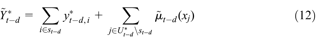
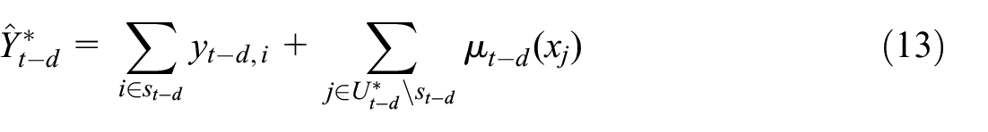
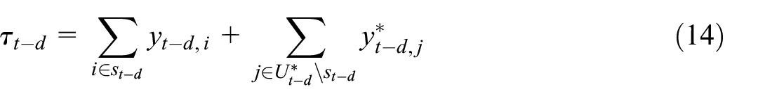
Let $I_t^{*}$ be the retrospectively observed index for month $t$ based on the totals ${\tau }_t$ given above, that is, using $\{y_{\mathrm{ti}}:i\in s_t\}\cup \{y_{\mathrm{tj}}^{*}:j\in s_t^c\}$ where $s_t^c=U_t^{*}\backslash s_t$ and $y_{\mathrm{ti}}^{*}$ is the VAT turnover value of unit $i$ in month $t$ . Let ${\hat{I}}_t$ be the corresponding flash RTI actually produced for month $t$ . For uncertainty assessment we aim to estimate a prediction interval for $I_t^{*}$ at a time when we only have ${\hat{I}}_t$ but not $I_t^{*}$ .

Since we observe ${\hat{I}}_t-I_t^{*}$ retrospectively, it is possible to consider the problem as one of time series forecasting provided a sufficient number of observations of ${\hat{I}}_t-I_t^{*}$ . This is, however, not the case here given the short history of debit card transactions data. Below we consider two feasible approaches.

2.5.1. Empirical Method

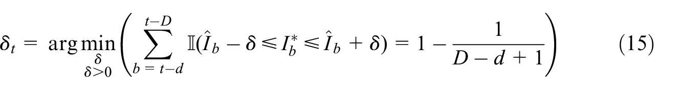
One can simply produce a prediction interval with calibrated empirical coverage over the most recent time window, denoted by $\{t-d,...,t-D\}$ . Let the prediction interval for month $t$ be given as

$$[{\widehat{I}}_t-{\delta }_t,{\widehat{I}}_t+{\delta }_t]$$

where

$${\delta }_t=\arg \underset{\begin{array}{c}\delta \\ \delta >0\end{array}}{\min }\left(\sum _{b=t-d}^{t-D}\mathbb{I}({\widehat{I}}_b-\delta \le I_b^{\ast }\le {\widehat{I}}_b+\delta )=1-\frac{1}{D-d+1}\right)$$

(15)

That is, ${\delta }_t$ is the minimum positive value of $\delta$ such that the interval $[{\hat{I}}_b-\delta ,{\hat{I}}_b+\delta ]$ achieves the specified coverage over the time window $b\in \{t-d,...,t-D\}$ .

For example, if $D-d+1=12$ , then the empirical coverage specified by (15) is 91.7%. Though simple, this empirical method is unlikely to be efficient because it does not make use of the VAT turnover values at the unit level.

2.5.2. Error Prediction

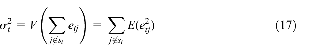
To fix the idea, let $\mu (x,s_t^{*})$ be obtained by augmented learning and $\mu (x_{\mathrm{tj}},s_t^{*})$ is the predicted turnover value in month $t$ for any $j\notin s_t$ . Let

$$e_{tj}=\mu (x_{tj},s_t^{\ast })-y_{tj}^{\ast }$$

(16)

be the error (against the VAT turnover value $y_{\mathrm{tj}}^{*}$ ) that can be observed with a delay. In case $\mu (x,s_t^{*})$ is an unbiased predictor and the prediction error is independent over the units outside of $s_t$ , we have

$${\sigma }_t^2=V\left(\sum _{j\notin s_t}{e}_{tj}\right)=\sum _{j\notin s_t}E(e_{tj}^2)$$

(17)

In order to estimate ${\sigma }_t^2$ at the population total level, we now devise an error prediction approach that can be viewed as a form of quasi transfer learning.

First, denote the unit-level $e^2$ -predictor by

$${\widehat{e}}^2=\eta (x,{\tilde{s}}_t^c)$$

(18)

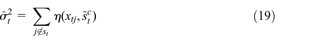
That is, a chosen model $\eta$ trained on the data associated with the units in ${\tilde{s}}_t^c$ , such that an estimate of ${\sigma }_t^2$ follows as

$${\widehat{\sigma }}_t^2=\sum _{j\notin s_t}\eta (x_{tj},{\tilde{s}}_t^c)$$

(19)

Next, for any $t$ , we can only train the model Equation (18) based on historical data, since the most recent VAT turnover value refers to month $t-d$ instead of $t$ . For a specific description, suppose the setups for outcome prediction of $y_{\mathrm{tj}}$ (by augmented learning) and error prediction of $e_{\mathrm{tj}}$ are such that

$$r_t^{\ast }={\tilde{s}}_t^c=R_{t^{\prime }}^{\ast }\cup R_{t-d}^{\ast }$$

Notice that the predictor Equation (18) trained on the observed errors for past time points is transferred to the current $t$ for error prediction, and the squared error $e_{\mathrm{bj}}^2$ is calculated against the VAT turnover value $y_{\mathrm{bj}}^{*}$ instead of the survey turnover value $y_{\mathrm{bj}}$ , where $b=t\prime$ or $t-d$ . Error prediction by (18) is therefore a form of quasi transfer learning.

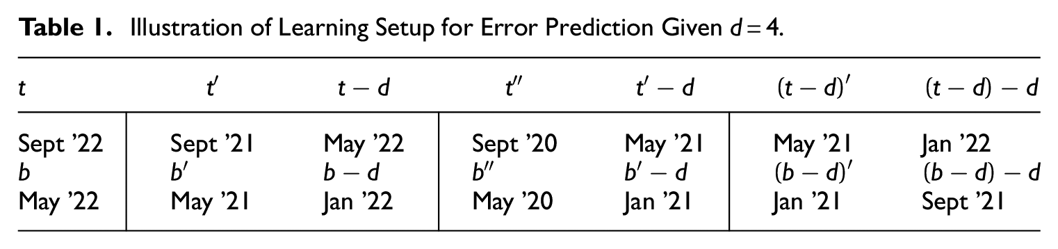
To illustrate, suppose $t=$ September 2022 (Table 1). Outcome prediction of $y_{\mathrm{tj}}$ by augmented learning uses $r_t^{*}$ containing the non-take-all units in September 2021 (i.e., $t\prime$ ) and May 2022 (i.e., $t-d$ ) given $d=4$ . Given the same setup of ${\tilde{s}}_t^c$ for associated error prediction by (18), the VAT turnover values needed to calculate the relevant $e^2$ -observations are from September 2021 and May 2022. Moreover, to obtain the predictor $\mu (x)$ for $t\prime$ , we need augmented learning using data from September 2020 (i.e., $t″$ ) and May 2021 (i.e., $t\prime -d$ ); whereas, to obtain that for $t-d$ , we need data from May 2021 (i.e., $(t-d)\prime$ ) and January 2022 (i.e., $(t-d)-d$ ). Similarly for month- $b$ flash estimation in Table 1.

Table 1.

Illustration of Learning Setup for Error Prediction Given $d=4$ .

$t$	$t\prime$	$t-d$	$t″$	$t\prime -d$	$(t-d)\prime$	$(t-d)-d$
Sept ’22	Sept ’21	May ’22	Sept ’20	May ’21	May ’21	Jan ’22
$b$	$b\prime$	$b-d$	$b″$	$b\prime -d$	$(b-d)\prime$	$(b-d)-d$
May ’22	May ’21	Jan ’22	May ’20	Jan ’21	Jan ’21	Sept ’21

Note that this setup for Equation (18) requires two years of data backwards from $t$ . While the demand on past data is greater compared to uncertainty assessment for the survey sampling estimator, it is much less than what would have been usual for a time series forecasting approach.

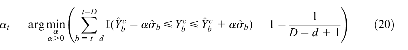
To derive a prediction interval using ${\hat{\sigma }}_t^2$ obtained in this way, let $Y_t^c=\sum _{j\notin s_t}{y}_{\mathrm{tj}}^{*}$ and let ${\hat{Y}}_t^c=\sum _{j\notin s_t}\mu (x_{\mathrm{tj}},s_t^{*})$ be its flash estimator. Similarly to Equation (15), an empirically coverage-calibrated prediction interval for $Y_t^c$ is given by

$$[{\widehat{Y}}_t^c-{\alpha }_t{\widehat{\sigma }}_t,{\widehat{Y}}_t^c+{\alpha }_t{\widehat{\sigma }}_t]$$

where

$${\alpha }_t=\arg \underset{\begin{array}{c}\alpha \\ \alpha >0\end{array}}{\min }\left(\sum _{b=t-d}^{t-D}\mathbb{I}({\widehat{Y}}_b^c-\alpha {\widehat{\sigma }}_b\le Y_b^c\le {\widehat{Y}}_b^c+\alpha {\widehat{\sigma }}_b)=1-\frac{1}{D-d+1}\right)$$

(20)

The corresponding prediction interval for $I_t^{*}$ can be derived straightforwardly given the observed total $\sum _{i\in s_t}{y}_{\mathrm{ti}}$ over $s_t$ in addition.

3. Application

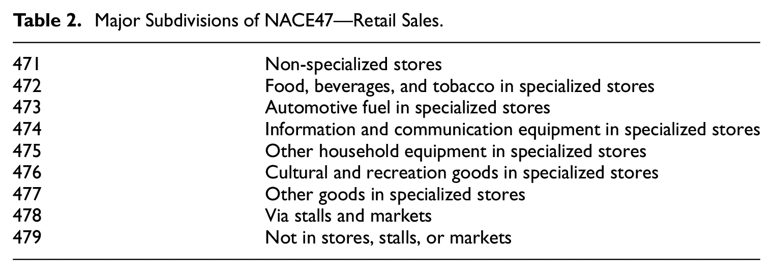
The NACE47 population has nine major domains (or subdivisions) by 3-digit NACE classification (Table 2). The domain NACE478 will be excluded here because it has separate data collection to the main survey.

Table 2.

Major Subdivisions of NACE47—Retail Sales.

471	Non-specialized stores
472	Food, beverages, and tobacco in specialized stores
473	Automotive fuel in specialized stores
474	Information and communication equipment in specialized stores
475	Other household equipment in specialized stores
476	Cultural and recreation goods in specialized stores
477	Other goods in specialized stores
478	Via stalls and markets
479	Not in stores, stalls, or markets

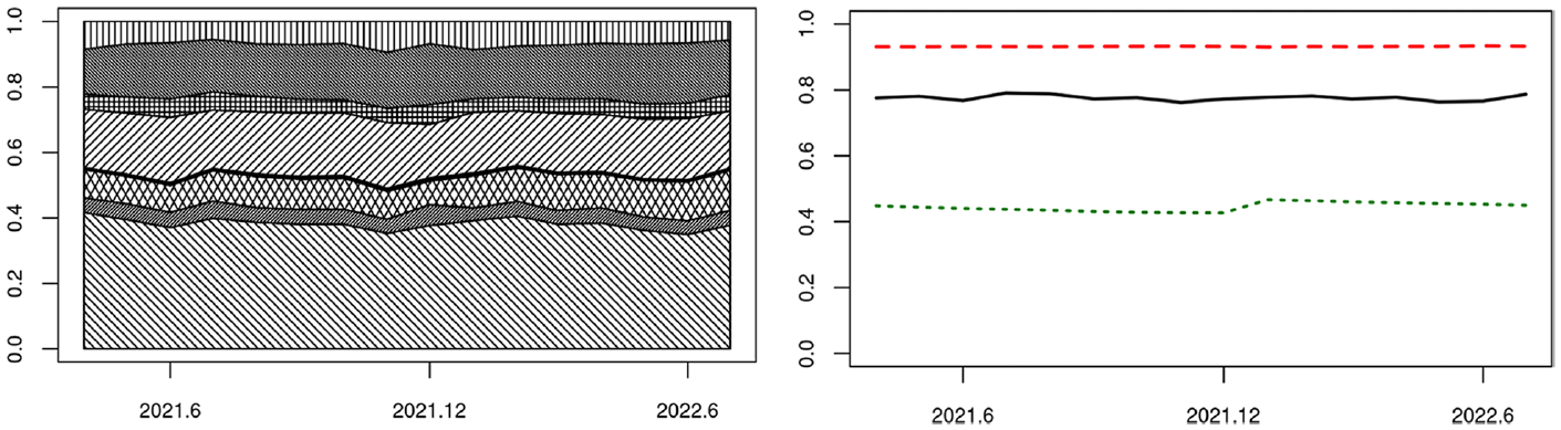
The left part of Figure 4 shows the estimated share of total turnover in the given period over 2021 and 2022, where each layer corresponds to one of the eight domains. The domain NACE471 including all the supermarkets has clearly the largest share of total turnover. The next two largest domains are NACE475 and NACE477. The smallest domain is NACE474.

Figure 4.

Left, estimated turnover share of eight domains of NACE47, each layer for a domain. Right, turnover share (solid line), sample proportion (dashed line), population proportion (dotted line) of take-all units. Period: April 2021 to July 2022.

The right part of Figure 4 shows the sample and population proportion of the take-all units over the same period, that is, $|s_t|/|s_t\cup r_t|$ and $|s_t|/|U_t|$ respectively, as well as their population share of the estimated total turnover, that is, $Y(s_t)/\hat{Y}(U_t)$ . The take-all units clearly command a dominant share of the total turnover in NACE47. This is an important premise for the traditional sample survey approach to RTI, as well as the potential success of flash estimation. In other words, the challenge would have been completely different, had one stopped surveying these units altogether.

Below we first show some detailed results comparing alternative models and learning approaches. Next, we report the flash estimates of the Norwegian RTI for NACE47, which are obtained by the chosen random forest model and augmented learning approach. Random forest is obtained by bootstrap aggregating (Breiman 1996a, 1996b) of tree models, where each tree model is generated by data-driven recursive partitioning of the feature space. See for example, Hastie et al. (2009) for more explanations of random forest models, as well as some other machine learning models that are potentially applicable. Our focus here is how to organize the available data for model learning, rather than how such models may be modified or improved themselves. Finally, retrospective validation and real-time uncertainty estimation are demonstrated.

3.1. Model and Learning Approach

For this part of the analysis we extracted the relevant data over 2021 and 2022. After various trials, we choose to let the feature vector of each unit contain its debit card payment total in month $t$ as well as its VAT turnover values in the most recent twelve months that are available at $t$ . The results to be reported below are not noticeably improved by including past transaction totals as features, but the results would have deteriorated to various extent over time had the concurrent transactions total been removed as a feature.

In particular, we notice that including a binary indicator for whether a unit belongs to $s_t$ or not would actually lead to worse prediction results.

Linear regression and random forest have been compared for all the choices of feature vector we have explored. Only the results obtained with the final choice of feature vector are given here to save space.

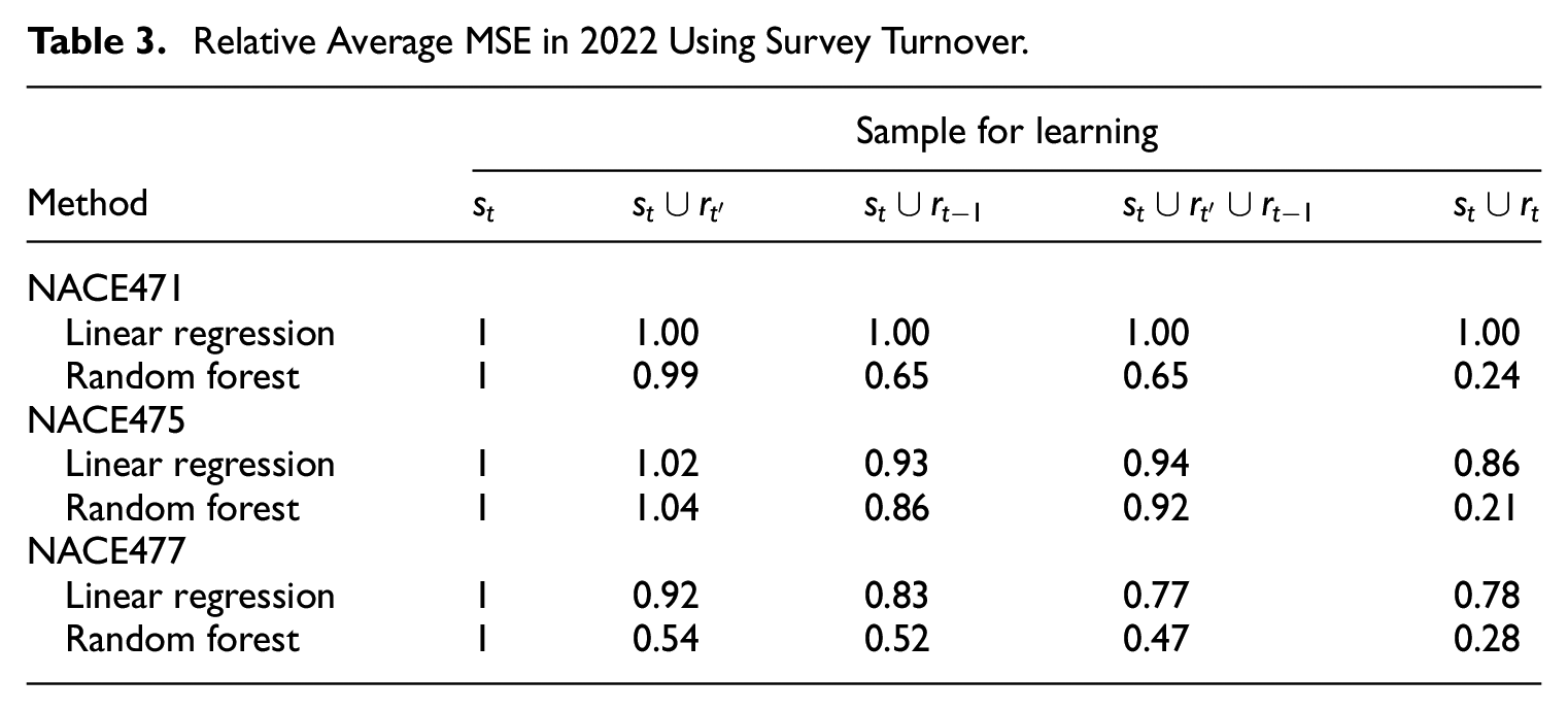
Setting-I. For each month $t$ , let the mean squared error (MSE) of a model be calculated from the take-some units in $r_t$ , that is, $\sum _{j\in r_t}\{\mu (x_{\mathrm{tj}})-y_{\mathrm{tj}}{\}}^2/|r_t|$ . Table 3 shows the average MSE over the twelve months of 2022 in the three largest domains, relative to that of the simplistic learning approach of only using $s_t$ . The three choices of $r_t^{*}$ in (6) are considered for augmented learning, as well as the hypothetical setting of training the models on $s_t\cup r_t$ as if they were all available for flash estimation. Although “mean squared residual” would have been a more appropriate term when a model trained on $s_t\cup r_t$ is applied to $r_t$ , we shall only use the term MSE for simplicity of description.

Table 3.

Relative Average MSE in 2022 Using Survey Turnover.

	Sample for learning
Method	$s_t$	$s_t\cup r_{t\prime }$	$s_t\cup r_{t-1}$	$s_t\cup r_{t\prime }\cup r_{t-1}$	$s_t\cup r_t$
NACE471
Linear regression	1	1.00	1.00	1.00	1.00
Random forest	1	0.99	0.65	0.65	0.24
NACE475
Linear regression	1	1.02	0.93	0.94	0.86
Random forest	1	1.04	0.86	0.92	0.21
NACE477
Linear regression	1	0.92	0.83	0.77	0.78
Random forest	1	0.54	0.52	0.47	0.28

Clearly, with suitable choice of $r_t^{*}$ , augmented learning by random forest can yield much greater reductions of MSE compared to linear regression in any of the NACE domains. Although the average MSE by augmented learning is larger than learning based on the true sample $s_t\cup r_t$ , augmented learning is able to improve the simplistic approach of only using $s_t$ .

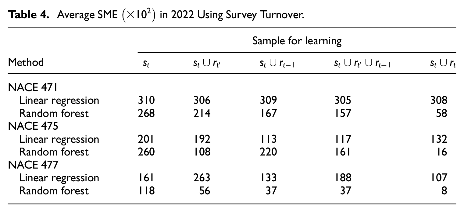
The squared mean error (SME), that is, $\{|r_t{|}^{-1}\sum _{j\in r_t}\mu (x_{\mathrm{tj}})-y_{\mathrm{tj}}{\}}^2$ , is more relevant for RTI than MSE. Table 4 shows the average SME over the twelve months of 2022 in the three NACE domains, by the same models and learning approaches. Random forest yields greatly reduced SME compared to linear regression in all the domains. Notice that the relative improvement of augmented learning to simplistic learning only from $s_t$ is more pronounced than in terms of MSE, for example, $37/118<0.47$ for the corresponding cells in the last row of Tables 3 or 4. Finally, the relative performance of training random forest on $s_t\cup r_t$ instead of $s_t\cup r_{t\prime }\cup r_{t-1}$ may have been exaggerated here, due to the use of residuals in the former case, since training the linear model (i.e., less prone to overfitting) does not always lead to as impressive SME reductions.

Table 4.

Average SME $(\times {10}^2)$ in 2022 Using Survey Turnover.

	Sample for learning
Method	$s_t$	$s_t\cup r_{t\prime }$	$s_t\cup r_{t-1}$	$s_t\cup r_{t\prime }\cup r_{t-1}$	$s_t\cup r_t$
NACE 471
Linear regression	310	306	309	305	308
Random forest	268	214	167	157	58
NACE 475
Linear regression	201	192	113	117	132
Random forest	260	108	220	161	16
NACE 477
Linear regression	161	263	133	188	107
Random forest	118	56	37	37	8

Setting-II. Augmented learning in setting-I above enables flash estimation without the sample units $r_t$ . Purposive sampling achieves further reduction of burden and resource, whereby the non-take-all units are dropped from the survey altogether. Since this also removes all the survey turnover observations of the cutoff units, augmented learning would depend on proxy values.

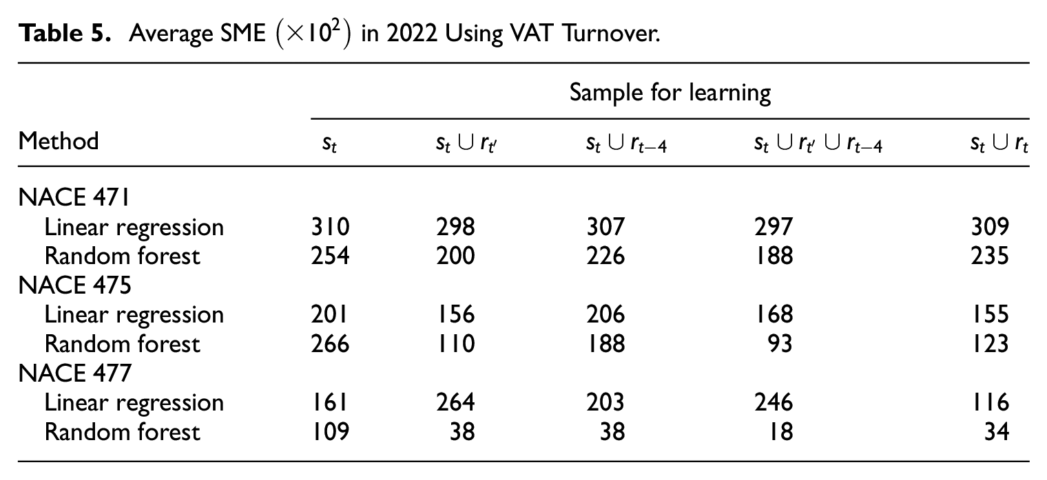
All the non-take-all VAT units can be used for augmented learning by Equation (7). However, here we shall present augmented learning based on past $r$ -samples associated with VAT turnover values instead of the observed survey turnovers, as well as in $r_t$ for the hypothetical setting of training on $s_t\cup r_t$ . Since the most recent VAT turnovers at $t$ refer to $t-d$ , we use $r_{t-4}$ instead of $r_{t-1}$ in $r_t^{*}$ given $d=4$ in Norway. In this way, the differences to the results above would only be due to the use of VAT turnovers that replace the survey turnovers, without the additional effects of including more units in $r_t^{*}$ .

The SME results are given in Table 5 in the same way as Table 4. Random forest remains much better than linear regression. Regarding the learning approach, we conclude the following for augmented learning.

• Augmented learning can reduce the SME compared to simplistic learning only from the take-all sample $s_t$ .

• Comparing Table 5 to 4, one sees that augmented learning from mixing contemporaneous survey turnover and historic VAT turnover can perform as well as augmented learning fully based on survey turnover observations. This provides a justification for purposive sampling.

• Training models on $s_t\cup r_t$ does not reduce SME compared to augmented learning using suitable $s_t\cup r_t^{*}$ , if VAT turnover is used as the $y$ -values in $r_t$ . Augmenting sample with past units is justified.

• In particular, the setup $s_t^{*}=s_t\cup r_{t\prime }\cup r_{t-4}$ seems to be a robust choice, which uses both the year-on-year and the most recent VAT-turnovers.

Table 5.

Average SME $(\times {10}^2)$ in 2022 Using VAT Turnover.

	Sample for learning
Method	$s_t$	$s_t\cup r_{t\prime }$	$s_t\cup r_{t-4}$	$s_t\cup r_{t\prime }\cup r_{t-4}$	$s_t\cup r_t$
NACE 471
Linear regression	310	298	307	297	309
Random forest	254	200	226	188	235
NACE 475
Linear regression	201	156	206	168	155
Random forest	266	110	188	93	123
NACE 477
Linear regression	161	264	203	246	116
Random forest	109	38	38	18	34

Quasi transfer learning. The scheme A requires transferring a past source model to the current time $t$ . It performs poorly for the same data above, which is not surprising given the dynamic nature of RTI. The results below are obtained by the scheme B, given either (11a) or (11b), where the target set is $q_t=s_t\cup r_t$ and the source time point is $b=t-1$ , and survey turnover values are used everywhere. The results are directly comparable to those of Table 4.

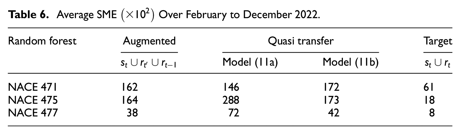
Since the sample $s_b^{*}$ for quasi transfer learning dates further back in time than $s_t^{*}$ for augmented learning, the results is only available for February to December 2022 based on the same data above. Table 6 shows the average SME over these eleven months, together with the results for augmented learning (using $r_t^{*}=r_{t\prime }\cup r_{t-1}$ ) and target learning (using $s_t\cup r_t$ ), which are comparable to those in Table 4 averaged over twelve months.

Table 6.

Average SME $(\times {10}^2)$ Over February to December 2022.

Random forest	Augmented	Quasi transfer		Target
	$s_t\cup r_{t\prime }\cup r_{t-1}$	Model (11a)	Model (11b)	$s_t\cup r_t$
NACE 471	162	146	172	61
NACE 475	164	288	173	18
NACE 477	38	72	42	8

It can be seen that the SME of the model Equation (11a) varies more across the NACE domains than that of the model Equation (11b). Quasi transfer learning using the model Equation (11b) yields slightly larger SME compared to augmented learning. It might be possible to fine-tune the choice of $b$ for the past source models (Figure 2), so as to improve the results of quasi transfer learning. However, given the relative simplicity and intuitiveness of augmented learning, we conclude that augmented learning is the preferred learning approach for flash RTI in Norway.

3.2. Flash RTI

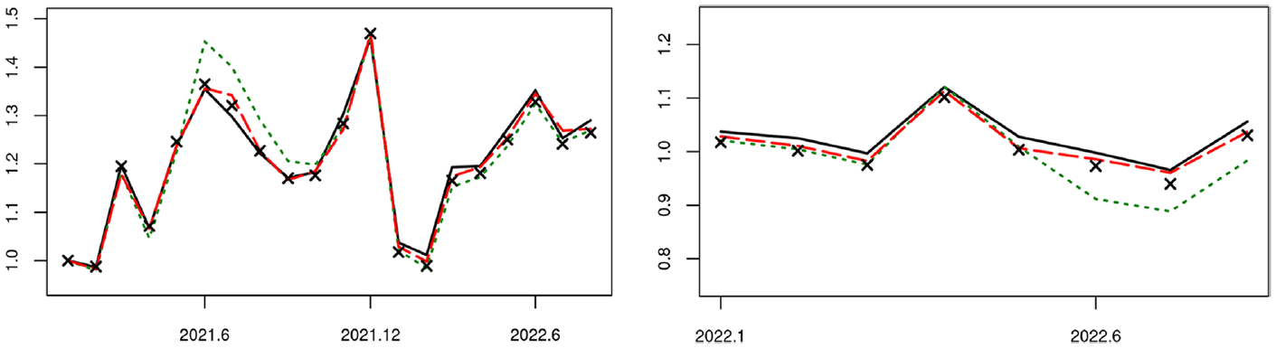
Figure 5 shows flash RTI estimation results for NACE47 (excluding NACE478) over the relevant months in 2021 and 2022, based on purposive sampling and using debit card transactions data, both in terms of the monthly and the year-on-year indices. The chosen random forest model is trained by augmented learning based on $s_t\cup R_{t\prime }\cup R_{t-4}$ , with associated $\{(x_{\mathrm{ti}},y_{\mathrm{ti}}):i\in s_t\}$ , $\{(x_{t\prime i},y_{t\prime i}^{*}):i\in R_{t\prime }\}$ , and $\{(x_{t-4,i},y_{t-4,i}^{*}):i\in R_{t-4}\}$ . In addition, the flash RTI by the simplistic learning only from $s_t$ is given, as well as the hypothetical flash RTI that uses the random forest model learned from $r_t$ to predict for $R_t$ .

Figure 5.

Existing RTI (solid line) for NACE47 over periods of 2021 to 2022, flash RTI by simplistic learning (dotted line), augmented learning (dashed line), or hypothetical learning from $r_t$ (cross line). Left: monthly index; right: year-on-year index.

The existing survey sampling approach requires both $s_t$ and $r_t$ and serves as the performance benchmark. It is seen that simplistic learning from only $s_t$ can sometimes deviate quite far from the disseminated RTI. The flash RTI obtained by augmented learning without $r_t$ achieves comparable performance to hypothetical learning from the target observations in $r_t$ , although in principle unbiased prediction is only possible with the latter but not the former.

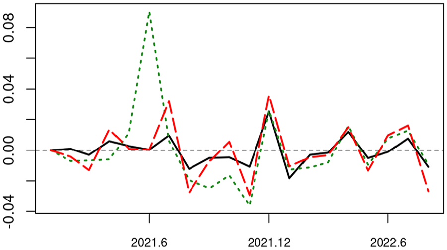
Moreover, let ${\hat{I}}_t$ be a given flash RTI for month $t$ and let $I_t$ the official RTI which is based on the existing sample survey design. Let the difference between the monthly change by the two be given as

$$B_t=({\widehat{I}}_t-{\widehat{I}}_{t-1})-(I_t-I_{t-1})=({\widehat{I}}_t-I_t)-({\widehat{I}}_{t-1}-I_{t-1})$$

(21)

Figure 6 shows $B_t$ for the three learning options in Figure 5. Although auto-correlations exist in all the three times series $\{I_t\}$ , $\{{\hat{I}}_t\}$ , $\{{\hat{I}}_t-I_t\}$ , respectively, one cannot detect any pronounced auto-correlation in the plot of $B_t$ .

Figure 6.

Difference of monthly change in flash RTI and official RTI for NACE47 over periods of 2021 to 2022. Simplistic learning (dotted line), augmented learning (dashed line), hypothetical learning from $r_t$ (solid line).

The results suggest that, by adopting an appropriate learning approach, one may be able to drop the take-some sample $r_t$ , reduce the response burden and the processing cost, and greatly improve the timeliness of RTI by halving the current dissemination time lag, without compromising the accuracy of RTI.

3.3. Validation and Uncertainty

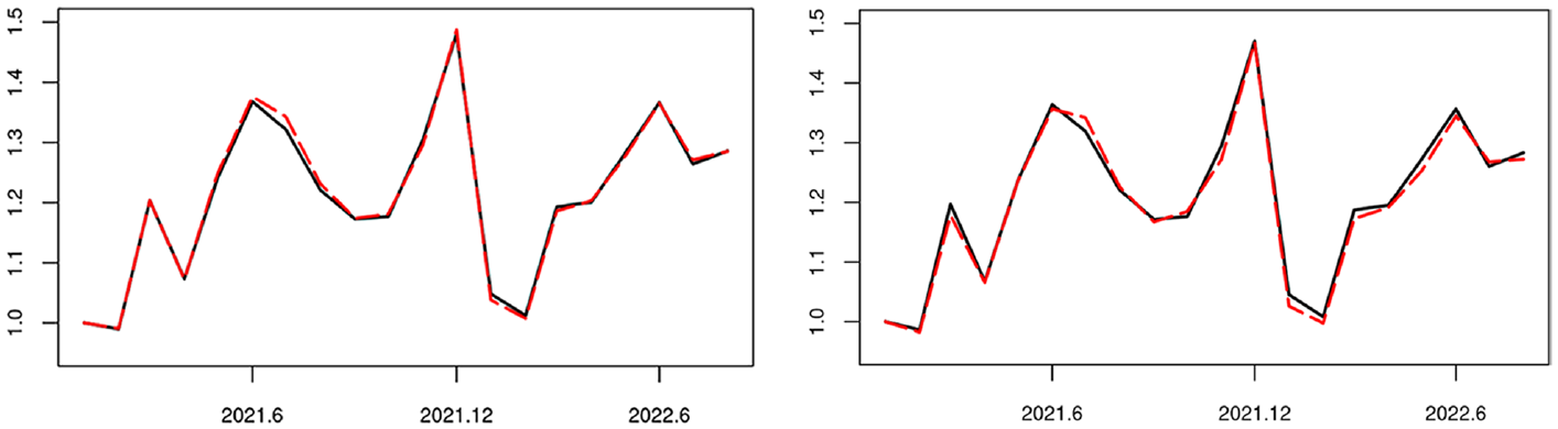
First, Figure 7 shows the results of retrospective validation as described in Subsection 2.4. The adopted random forest model for flash RTI (described above) is fitted to the population of VAT units $U_t^{*}$ relevant to each $t$ , which yields the model-predicted VAT index derived from ${\tilde{Y}}_t^{*}$ (dashed) in the left plot of Figure 7. It can be seen that the model fits the VAT population quite well over the period here, since the discrepancy between the model-predicted VAT index and the VAT index derived from the observed $Y_t^{*}$ (solid) is barely noticeable in the given period except perhaps for July 2021.

Figure 7.

Retrospective validation of flash RTI given in Figure 5. Left, random forest model, VAT index observed (solid line) or model-predicted (dashed line). Right, augmented learning, proxy-RTI index observed (solid line) or learned (dashed line).

In the right plot of Figure 7, the adopted random forest model is trained by augmented learning (as for the flash RTI), which yields the learned index derived from ${\hat{Y}}_t^{*}$ (described in Subsection 2.4). It tracks closely its target proxy-RTI index derived from ${\tau }_t$ , although augmented learning does seem to induce some discrepancy in addition to that due to modeling (in the left plot).

It is important to notice that the discrepancy between the learned index (of ${\hat{Y}}_t^{*}$ ) and the proxy-RTI index (of ${\tau }_t$ ) in Figure 7 reflects well the discrepancy between the flash RTI (by augmented learning) and the disseminated RTI (by existing survey sampling) in Figure 5. The proposed retrospective validation approach can provide a reliable basis for assessing whether the flash RTI has worked satisfactorily till as recently as $d$ months ago.

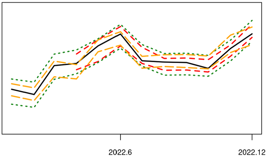
Next, for uncertainty estimation, Figure 8 shows the VAT total that is only available retrospectively (i.e., $Y_t^c$ in Subsection 2.5), together with its prediction intervals by the empirical or error prediction method and its confidence intervals by survey sampling. Whereas the intervals by the empirical method Equation (15) and survey sampling are obtained for all the twelve months of 2022, we could only calculate the intervals for April to December by the error prediction method Equation (20) given the data available, because this method requires more data backwards under the adopted setup of augmented learning.

Figure 8.

VAT total (solid line), prediction interval by empirical method (dotted line) or error prediction (dashed line), confidence interval by sampling (long-dashed line).

The prediction intervals are empirically calibrated by either Equation (15) or Equation (20) to the nominal level 91.7% based on a sliding window of twelve months. The nominal level of the confidence intervals by survey sampling is 95%, which are obtained as follows. Let ${\tilde{Y}}_t^c$ be the ratio estimator based on the existing subsample $r_t$ , which uses the VAT values from the same month in the previous year as the auxiliary. Let ${\mathrm{se}}_t$ be the estimated standard error of this ratio estimator. We obtain an approximate 95% confidence interval $({\tilde{Y}}_t^c-2{\mathrm{se}}_t,{\tilde{Y}}_t^c+2{\mathrm{se}}_t)$ by appealing to the Central Limit Theorem.

The actual coverage is 100% by both of the prediction intervals during their respective periods in 2022. The coverage of the 95% confidence intervals based on survey sampling is 91.7%, which are not calibrated empirically as we do for the prediction intervals. Notwithstanding the fairly short time span of these results, the proposed prediction intervals display promising coverage property. As can be expected, error prediction modeling Equation (18) improves considerably the efficiency of estimation compared to the simple empirical method, where the average relative half-length (of prediction interval) is 4.7% by error prediction Equation (18) and 7.8% by the empirical method Equation (15).

Since the average relative half-length of the confidence intervals by ratio estimation is 4.6%, flash estimation without subsample $r_t$ has been about as efficient as the sampling-based ratio estimation that requires $r_t$ . It seems fair to conclude that augmented learning can enable flash estimation with greatly improved timeliness, as well as reduced response burden and processing cost, without compromising the accuracy of RTI.

4. Final Remarks

We have considered a setting for flash estimation, where target observations necessary for unbiased prediction are not available at all outside a purposive sample selected with probability one. Rather than simply applying a model learned from the purposive sample to the rest population units, we propose two general approaches of model learning that make use of data from relevant domains outside the target population, called augmented learning and pseudo transfer learning, respectively. Moreover, retrospective validation of modeling or learning and real-time prediction interval estimation methods are developed in the context of Turnover Statistics.

Application to the Norwegian Retail Turnover Survey data shows that it is possible to obtain flash RTI for NACE47 based on augmented learning, which greatly improves the timeliness by halving the current dissemination time lag, without compromising the accuracy of RTI. The adopted model utilizes relevant auxiliary information in historic VAT reports and contemporaneous debit card transactions, enabling one to remove the non-self-representing sample units, thereby reducing the associated response burden and processing cost.

The flash RTI methodology described above and the related production processes are being implemented at Statistics Norway. Three broad, interrelated aspects are worth noting for other countries with a similar interest.

First, greater uses of historic VAT reports can benefit from improvements of the underlying statistical database. For instance, the bimonthly VAT reports have been apportioned to create a statistical database of monthly VAT turnover values for the local units which can be used for flash RTI estimation, the details of which have been left out to save space. Similar apportioning of available VAT register data may be relevant in other countries, in order to harmonize over the different frequencies and units of VAT reporting that exist. The resulting statistical database is more “complete” and “detailed” than the raw VAT register, which can benefit many relevant statistics.

Second, we have made use of debit card transactions that are available to Statistics Norway, which fundamentally improves the timeliness of auxiliary information compared to the VAT register that is only available months later. Other sources of transaction data are also of interest, such as e-invoices and business-to-business bank transfers. While the different sources have their distinct challenges of access and processing, they complement each other in coverage and content, becoming more useful in combination with each other. This is an area that requires strategic development of knowledge, experience and capacity at National Statistical Offices. A coordinated program across the whole spectrum of business statistics would be more impactful than scattered efforts each focusing on a specific topic.

Third, provided greater access to relevant and timely non-survey big data, improving the timeliness of economic indicators while reducing the response burden and processing cost becomes an ever more urgent matter. The flash RTI exemplifies a situation where some survey data is still necessary to ensure the relevance and accuracy of official statistics. Combining appropriate purposive samples with novel modeling and learning approaches requires attention in practice. Diligent retrospective validation is essential in this respect, in terms of the adopted model, learning approach, as well as the associated uncertainty measures such as prediction intervals. The obtained insights should help to guide the maintenance and updating of the purposive sample, in order to be able to compensate for the data that are either missing structurally (such as when the take-some sample is removed altogether) or randomly (e.g., due to delays of reporting, new or dissolved business units).

Looking ahead we would like to point toward a greater emphasis on novel learning approaches for official statistics. In the context of flash estimation, where the absence of target observations is the fundamental challenge, a key matter of learning is how to organize the data outside the target domain but are nevertheless relevant (for training any given models). Augmented learning and quasi transfer learning have been proposed from this perspective. As official statistics are typically repeated over time and geography, variations of transfer learning (with or without target observations) seems a large topic for future research and application, for example, beyond the common traditional approach of allowing for temporally or spatially correlated observations.

References

1.
BaldacciE.BuonoD.KapetaniosG.KrischeS.MarcellinoM.MazziG. L.PapailiasF.2016. Big Data and Macroeconomic Nowcasting: From Data Access to Modelling. Luxembourg: Eurostat: Statistical Books. DOI: https://doi.org/10.2785/3605875.
2.
BreimanL.1996a. “Heuristics of Instability and Stabilization in Model Selection.”The Annals of Statistics24: 2350–83. DOI: https://doi.org/10.1214/aos/1032181158.
Eurostat. 2017. Handbook on Rapid Estimates. Edited by MazziG. L.Luxembourg: European Union and the United Nations. DOI: https://doi.org/10.2785/4887400.
5.
FornaroP.LuomarantaH.2020. “Nowcasting Finnish Real Economic Activity: A Machine Learning Approach.”Empirical Economics58: 55–71. DOI: https://doi.org/10.1007/s00181-019-01809-y.
6.
GuT.HanY.DuanR.2023. “A Transfer Learning Approach Based on Random Forest with Application to Breast Cancer Prediction in Underrepresented Populations.”Pacific Symposium on Biocomputing28: 186–97. https://pubmed.ncbi.nlm.nih.gov/36540976/.
7.
HastieT.TibshiraniR.FriedmanJ.2009. The Elements of Statistical Learning, 2nd edition. New York: Springer.
8.
LiS.CaiT. T.LiH.2020. “Transfer Learning for High-Dimensional Linear Regression: Prediction, Estimation, and Minimax Optimality.”Journal of the Royal Statistical Society: Series B (Statistical Methodology)84: 149–73. DOI: https://doi.org/10.1111/rssb.12479.
PrattL. Y.1993. “Transferring Previously Learned Back-Propagation Neural Networks to New Learning Tasks.” PhD thesis, Rutgers University, also appeared as Technical Report ML-TR-37. https://dl.acm.org/doi/book/10.5555/193298.
11.
TibshiraniR.1996. “Regression Shrinkage and Selection via the Lasso.”Journal of the Royal Statistical Society: Series B (Statistical Methodology)58: 267–88. DOI: https://doi.org/10.1111/j.2517-6161.1996.tb02080.x.