
Abstract
We consider the problem of estimating a time series of population means from a series of sample surveys when the means are known to be nondecreasing. We introduce the standard survey estimators of the series of means, which are not guaranteed to be nondecreasing. We employ the Pool Adjacent Violators Algorithm (PAVA) to turn the series of standard survey estimates into a nondecreasing series. We introduce five methods of constructing confidence intervals for the series of non-decreasing means: normal-theory intervals based on the standard survey point estimator of the mean and the Taylor series estimator of its variance; normal-theory intervals based on the nondecreasing PAVA estimator of the mean and a unique jackknife estimator of its variance developed here (jackknife-
1. Introduction
A common problem in survey research is to estimate a time series of population means based on periodic sample surveys. The main objective of this article is to develop and explore the statistical properties of confidence intervals for the population means when they are known or assumed to be monotonically nondecreasing for all time periods. Several authors have addressed similar problems in the context of dose-response studies—including Korn (1982), Morris (1988), and Dilleen et al. (2003)—and the methods of these authors may be adapted to the survey-research setting assumed in this article. Examples of the monotonic property include estimation of the proportion of the population of adults ever experiencing flu-like symptoms in the current flu season, the proportion of children in a given birth cohort who are up-to-date for the recommended schedule of vaccines (Centers for Disease Control and Prevention 2024), or the proportion of adults in a given cohort who have graduated from college.
We consider a time series of survey populations
Without loss of generality, we assume a weekly time series throughout this article. We assume delivery of the survey estimates is performed on the same period as the surveys. Thus, at the close of the current week, say
We assume each of the weekly populations is partitioned into
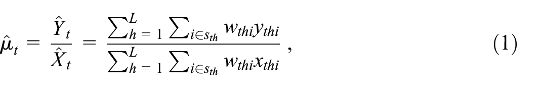
which is of the ratio form, where
A common practice in survey research is to estimate the variance of the standard estimator using either the Taylor series method or some form of replication, and to employ symmetric normal-theory confidence intervals for each of the population means in the series. Variances are estimated at each time point
Although
Users of the survey series may be disconcerted by random fluctuation in the standard estimates and gain greater confidence in the useability of the estimates if the estimates meet their expectations of monotonicity. Toward this end, isotonic regression is a nonparametric method for fitting a flexible curve to the estimated weekly means
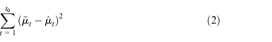
subject to the constraint
Estimating the variances of the monotonic values
Section 2 is a methods section in which we define the monotonic estimators and alternative confidence intervals and describe the design of the Monte Carlo study. Section 3 contains the results of the simulations, and the article concludes in Section 4 with discussion of the results and recommendations for point and interval estimation.
2. Methods
2.1. A Method of Mean Estimation That Honors Monotonicity
The Pool Adjacent Violators Algorithm (PAVA) solves the constrained minimization problem Equation (2). See Ayer et al. (1955), de Leeuw et al. (2009), and the references cited therein. A violation of the nondecreasing property occurs whenever
PAVA has been implemented in both the gpava function within the
2.2. Confidence Intervals for the Monotonic Series
We define five methods of constructing confidence intervals, which we examine later in Monte Carlo simulations. The first method entails a symmetric normal-theory confidence interval for the weekly population mean in which the point estimate is the standard estimate
The second and third methods for interval estimation are to employ symmetric confidence intervals from normal-theory and from Student’s t-distribution, centered at the monotonic estimator
for all
and the corresponding jackknife estimator of its variance (Wolter 2007, chap. 4) is
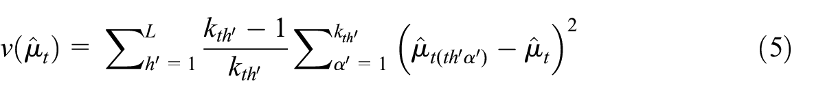
The specific instance of
While Equation (5) is the jackknife estimator of variance for the standard survey estimator of the population mean at week
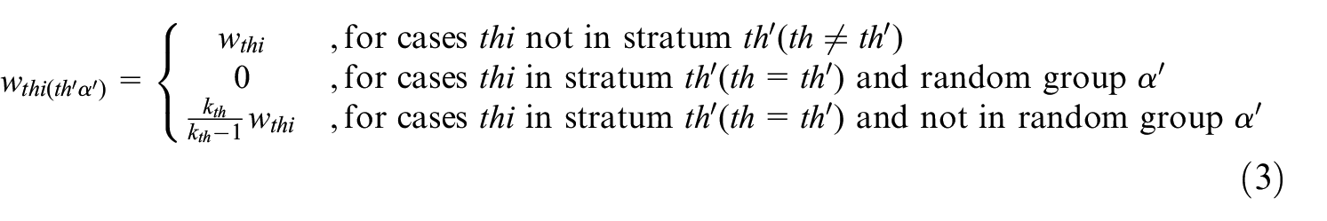
Considering these circumstances surrounding the PAVA series, we recognize all
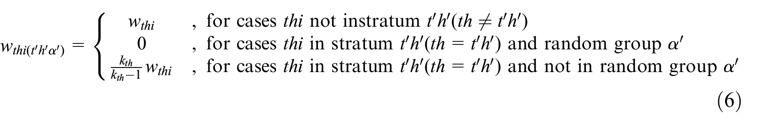
for all
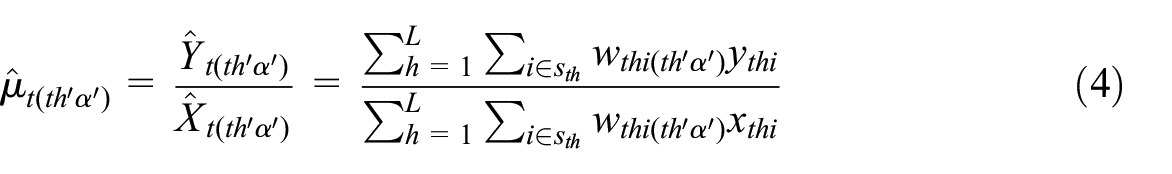
The standard survey series corresponding to the
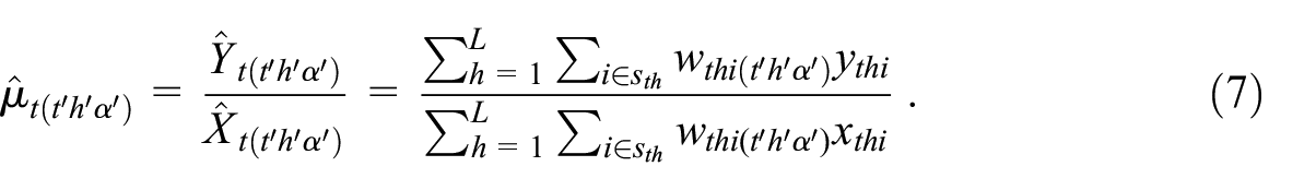
The survey estimator Equation (7) is the same as the survey estimator Equation (4) whenever the estimation week
Having defined the standard survey series corresponding to the jackknife replicates, we can turn to the PAVA series corresponding to jackknife replicates and to the jackknife estimator of variance. Specifically, the PAVA series corresponding to the
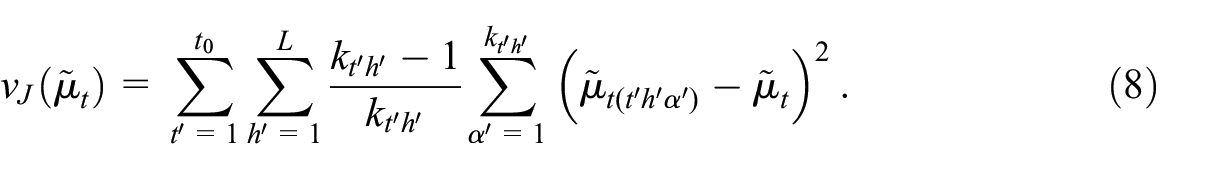
The corresponding jackknife confidence interval for the monotonic population mean is now
Morris (1988) developed the fourth method of interval estimation. His method deals with confidence intervals for a series of population proportions assuming simple random sampling with replacement from the populations indexed by
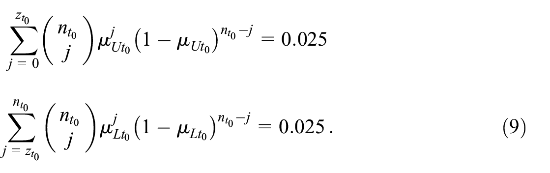
To produce 95% confidence limits for the monotonic series, the procedure starts by accepting the Clopper-Pearson upper confidence limit for the last proportion in the estimation window,
Given his assumptions, Morris proves that the resulting confidence limits are conservative, that is, the true confidence interval coverage probability is greater than or equal to the nominal value
The fifth and final method of interval estimation for the monotonic series, due to Korn (1982), also starts with the assumption of simple random sampling with replacement at each week. Absent the assumption of monotonicity, a 95% normal-theory confidence interval for the population proportion at week
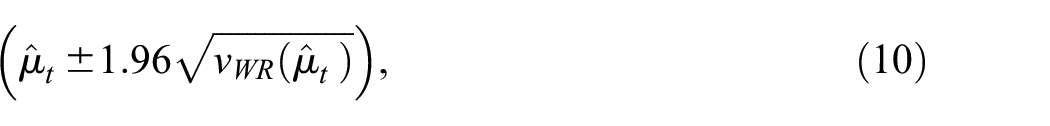
where the with-replacement estimator of variance is
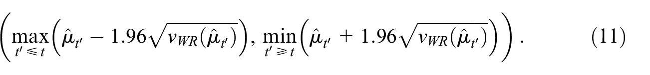
The limits are not derived from the PAVA estimators, but instead are directly derived from the standard estimator (1) of the population means. Although the confidence intervals Equation (11) are exact, given Korn’s assumptions, there is no guarantee they contain the PAVA values
2.3. Simulation Design and Metrics
In Section 3, we report the results of a Monte Carlo simulation conducted to investigate the statistical properties of the monotonic estimators and the Taylor, jackknife-
Our study includes eighteen populations designed to investigate performance under three varying factors: (1) non-decreasing series shapes (linear, concave, logistic), (2) series rates of increase (low, high), and (3) series sample sizes (low, medium, high). The three factors combine to reflect various signal-to-noise ratios in the standard series
The three shape functions are defined in Table 1. The model parameters,
Specification of Three Shape Functions for a Monte Carlo Study of Confidence Intervals for a Nondecreasing Series of Population Proportions.
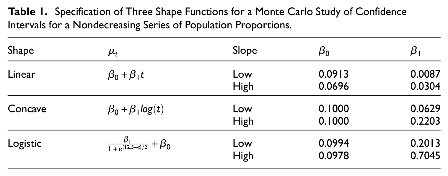
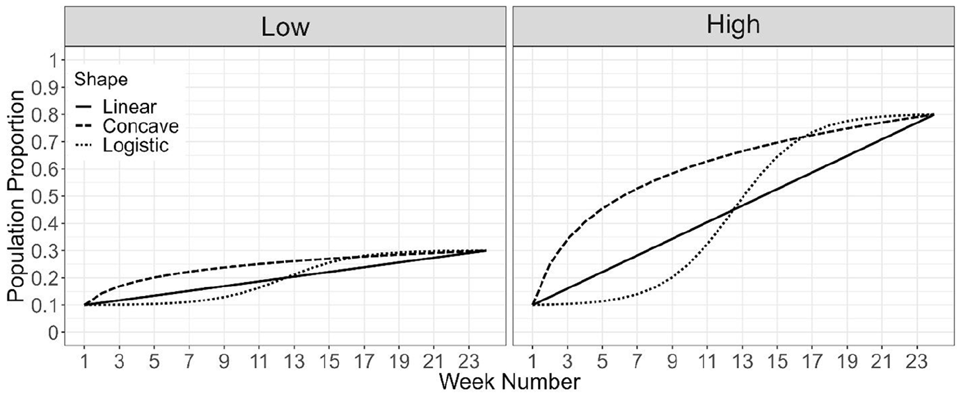
Illustration of population proportions by slope and shape.
We generated weekly samples of sizes
For each of the eighteen populations, we prepared the series of standard estimates
For the jackknife-
3. Monte Carlo Results
3.1. Preliminaries
Our results begin with a visualization of the data and an analysis of the average bias in the standard and PAVA series. Figure 2 plots the standard and PAVA series for each of the eighteen populations based on the first Monte Carlo replicate. (We plot the first replicate as an illustration of our data. Plots for other replicates would appear similar to these plots.) Columns in the figure reveal the three weekly sample sizes 24, 48, and 96; rows depict the low and high rates of increase; and blocks represent the linear, concave, and logistic shapes. The 95% confidence intervals based on the normal-theory jackknife-z approach are depicted in gray, while the wider Taylor confidence intervals are shown in blue. Morris and Korn intervals are depicted by the dotted and dashed black lines, respectively. Note that jackknife-
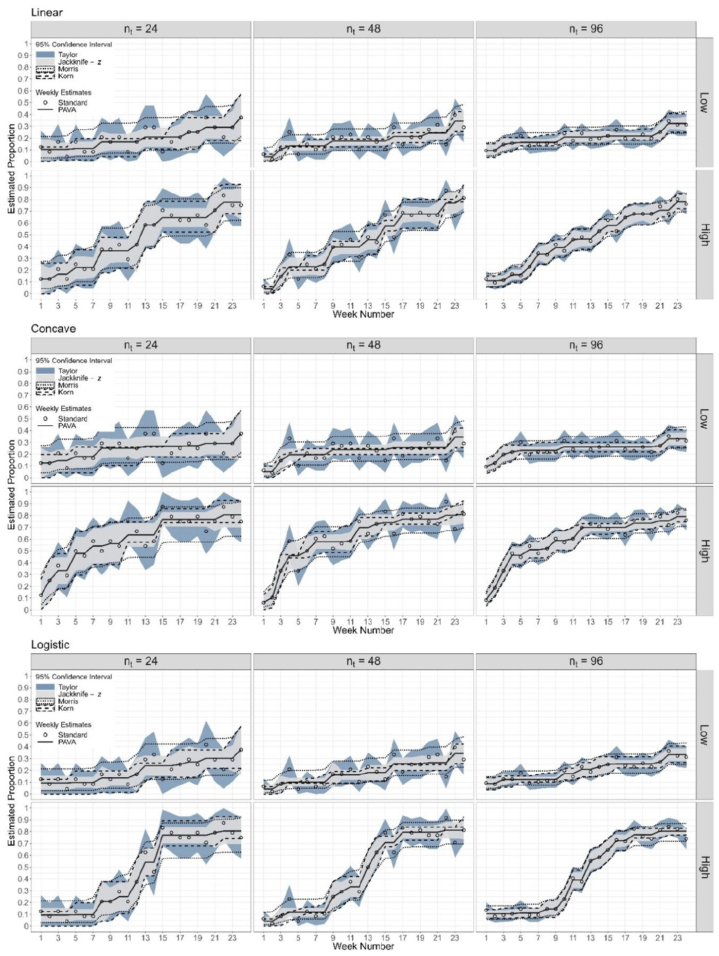
Plots of standard and PAVA series for eighteen populations and for the first Monte Carlo replicate.
As shown in Figure 2, the standard series of estimated proportions exhibit random fluctuation and are clearly not monotonic, while the PAVA series are monotonic, as expected. The jackknife intervals are narrower than the Taylor intervals, because the latter intervals ignore the fact or assumption of monotonicity and the smoothing of estimates brought by PAVA estimation. The Morris intervals appear narrower than the Taylor intervals but are wider than the jackknife intervals. The widths of the Korn intervals are comparable to both jackknife-
Prior to reporting the simulation results, we assess Monte Carlo Error (MCE) associated with the simulations, to inform the reader of the degree of uncertainty in the simulation results. Following the formula provided by Koehler et al. (2009), MCE is the standard deviation of the Monte Carlo estimator. Given a sample of 1,000 replicates generated under the design described in the previous section, we calculated the maximum MCE over all the simulation settings and all the estimators except for Korn estimator, given how different its coverage is from the other estimators. The maximum MCE is 0.33 percentage points for average bias estimation, 1.28 percentage points for coverage probability estimator, and 0.19 percentage points for half-width estimations.
Now, turning to the results of the simulations, Table 2 presents the Monte Carlo estimates of bias in the standard and PAVA series averaged over twenty-four weeks for each of the eighteen populations. Note that, by construction, the sum of the PAVA estimates across the weeks equals the sum of the standard estimates. Thus, the average theoretical bias of the PAVA estimator is the same as the average theoretical bias of the standard estimator, namely 0.0 across the twenty-four weeks. For example, for the population defined by the linear shape, low rate of increase, and weekly sample size of 48, the average bias as measured by 1,000 Monte Carlo replicates is −0.009 for both the PAVA and standard estimator. Thus, the table essentially verifies through simulation what is known from theory, that the average bias in the standard estimator is 0.0.
Average Bias (in Percentage Points) of Both the Standard and PAVA Series Across Twenty-Four Weeks by Shape, Rate of Increase, and Weekly Sample Size.
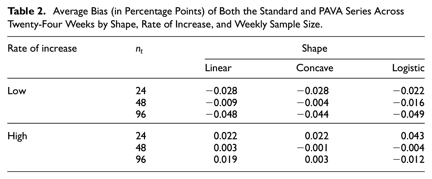
Figure 3 illustrates the bias by week in the PAVA series for the different shapes (column) and rates of increase (row) for all sample sizes. The figure reveals that the PAVA estimates are biased upward at the end of the series and downward at the beginning. For example, for the population in which the series has a low rate of increase and follows a logistic curve, the bias ranges from −3 percentage points at the beginning of the series to +5 percentage points at the end.
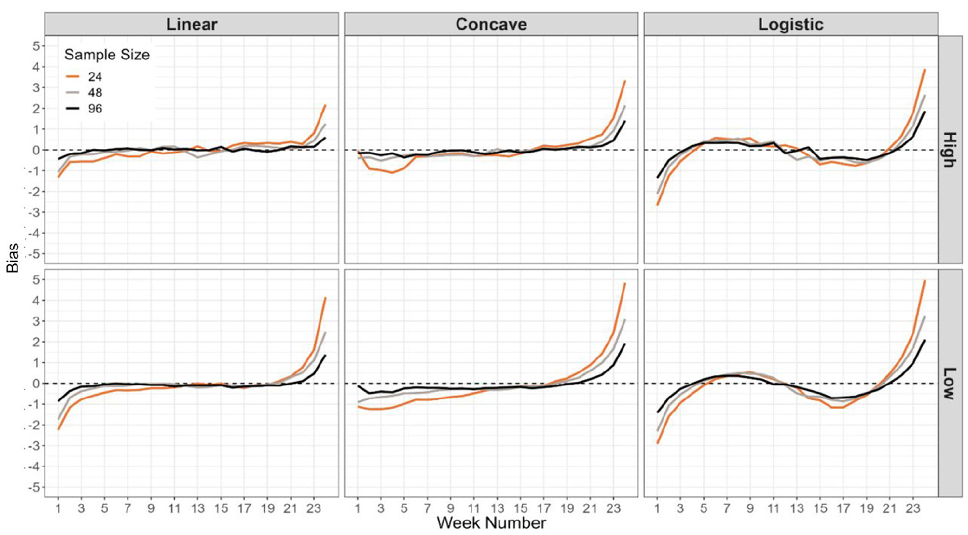
Bias (in percentage points) in the PAVA estimates versus week for various series shapes (column), rates of increase (row), and sample sizes.
The PAVA estimate at the end of the series is equal to or greater (when there is a violation) than the standard estimate, which is known to be unbiased. Similarly, at the beginning of the series, the PAVA estimate is equal to or less (when there is a violation) than the standard estimate. Thus, the PAVA estimator tends to be biased upward at the end of the series and tends to be biased downward at the beginning of the series except when the slope is very steep at the beginning or end, such as the concave series.
Finally, the estimator is slightly biased for the interior time points, though the magnitude of the bias decreases as sample size increases. The bias pattern also varies depending on the underlying shape of the series that impacts the rates of increase or slope at a given week. For example, the slope is the highest for the concave series and lowest for the logistic series near the series beginning. The bias magnitude is inversely related to the slope; thus, near the series beginning, the bias magnitude is the lowest for the concave series and the highest for the logistic series.
3.2. Confidence Interval Results
In this section, we assess the quality of the five confidence interval methods for population proportions in terms of their coverage probabilities, half-widths, and containment of the PAVA estimates.
3.2.1. Confidence Interval Coverage Probabilities
Table 3 presents Monte Carlo coverage probabilities for the 95% confidence intervals based on the five methods of interval estimation, for each of the eighteen populations, averaged over the twenty-four weeks within the estimation window.
Coverage Probabilities (in Percent) of the Five Confidence Interval Methods for the Population Proportion for Eighteen Populations, Averaged Across Twenty-Four Weeks.
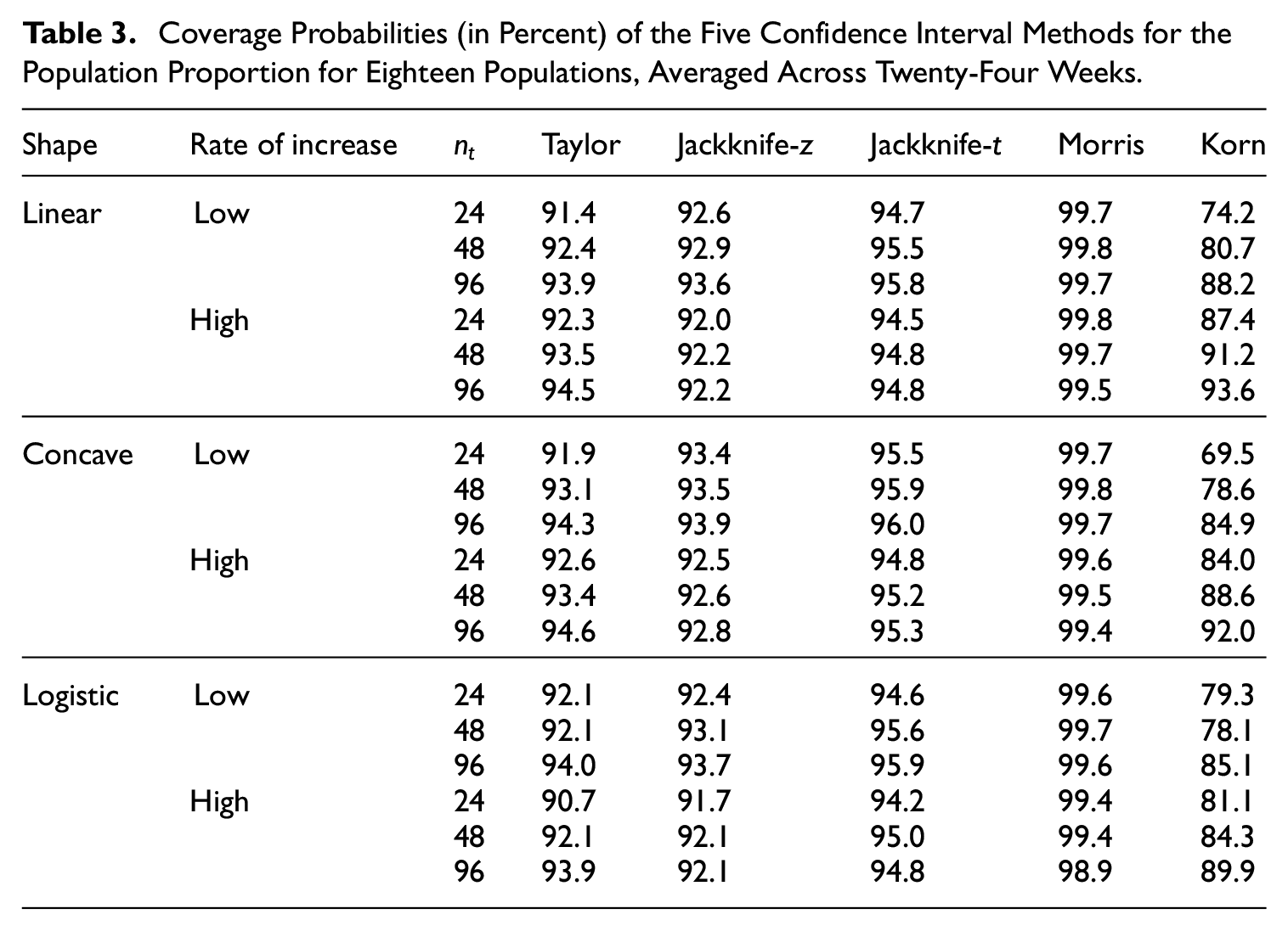
As one would expect from theory and experience, the coverage probabilities converge toward the nominal value of 95% as the sample size increases for the Taylor intervals. The two jackknife intervals account for the monotonicity and smoothness gained by PAVA, generating jackknife-
Coverage probabilities are slightly lower for the logistic shape than for the linear and concave shapes, likely because the logistic shape has more weekly population proportions near the boundaries (i.e., near 0 and 1), conditions in which normal-theory confidence intervals are known to exhibit relatively poor coverage (Brown et al. 2001). Furthermore, the average absolute bias is also higher for the logistic shape compared to the other shapes as illustrated in Figure 3. Overall, the coverage probabilities improve toward the nominal value of 95% as both the population rate of increase and the sample size increase.
In Figure 4 we examine confidence interval coverage probabilities by week for the different population shapes (column) and rates of increase (row), averaged over sample sizes. The Taylor and jackknife-
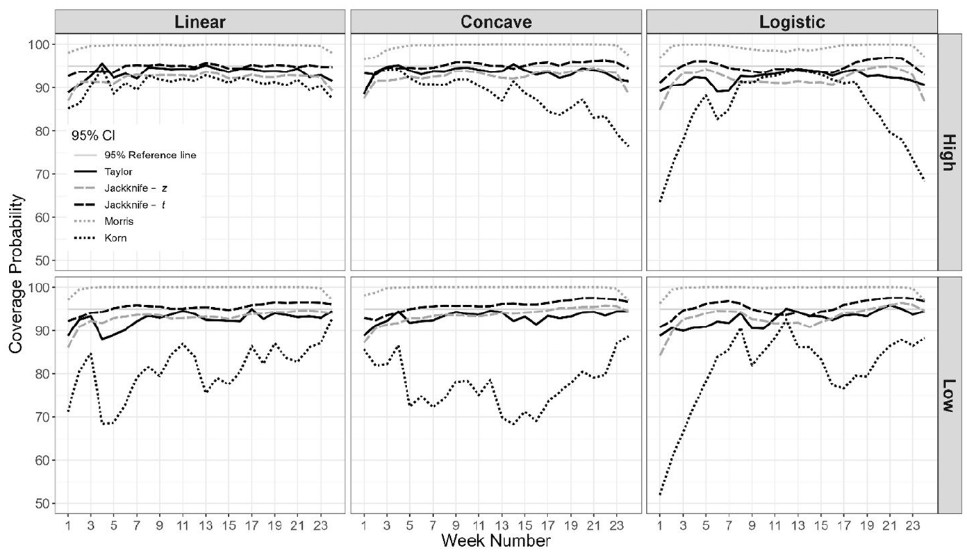
Coverage probabilities (in percent) of the five confidence interval methods versus week for populations defined by shape (column) and rate of increase (row), averaged over sample size.
For the Morris approach, coverage probabilities are all near 100%, while for the Korn intervals, coverage probabilities tend to be below 90%. The Korn approach appears to be sensitive to the signal-to-noise ratio, as shown by the low coverage probabilities when (1) the series of population proportions has a low rate of increase within the estimation window or (2) the series is relatively flat, such as near the beginning and end points of the logistic series and near the end point of the concave series. Finally, for each of the confidence-interval methods, weekly coverage probabilities tend to be lowest at the beginning and end points of the series, which is likely due to the bias in the PAVA estimates at the end points.
3.2.2. Confidence Interval Half-Widths
Table 4 presents average half-widths of 95% confidence intervals based on the five methods of interval estimation for each of the eighteen populations. The average half-widths range from 7 to 18 percentage points for the Taylor intervals, which are the widest intervals produced by any of the five methods. The jackknife-
Half-Widths in Percentage Points (i.e., the Original Scale Multiplied by 100) of the Five Confidence Interval Methods for the Population Proportion for Eighteen Populations, Averaged Across Twenty-Four Weeks.
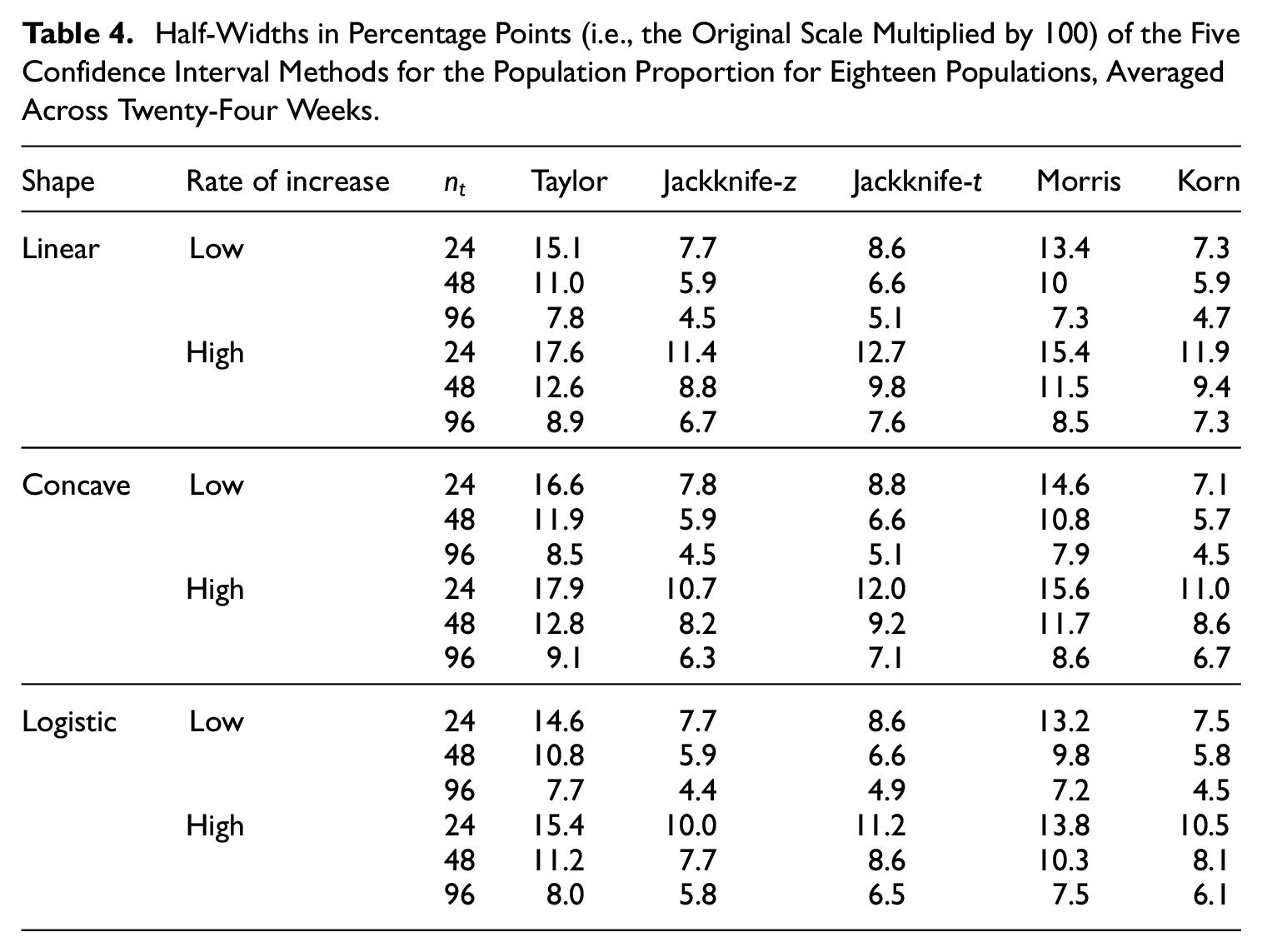
The Korn method generates half-widths that are slightly narrower compared to the jackknife-
Figure 5 compares the half-widths of the 95% confidence intervals by week for the populations defined by shape and rate of increase, averaged over sample size. The results by week are consistent with the results averaged across weeks reported in Table 4. Taylor intervals are wider than Morris intervals for all weeks, while the jackknife methods produce substantially narrower intervals. Korn intervals are also relatively narrow and comparable to the widths of the jackknife intervals. These patterns are consistent across populations defined by shape and rates of increase.
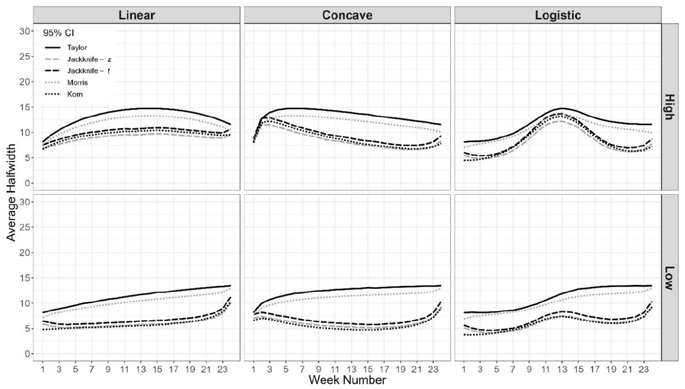
Half-widths in percentage points (i.e., the original scale multiplied by 100) of the five confidence interval methods versus week for populations defined by shape (column) and rate of increase (row), averaged over sample size.
3.2.3. Confidence Intervals That Do Not Contain the PAVA Estimate
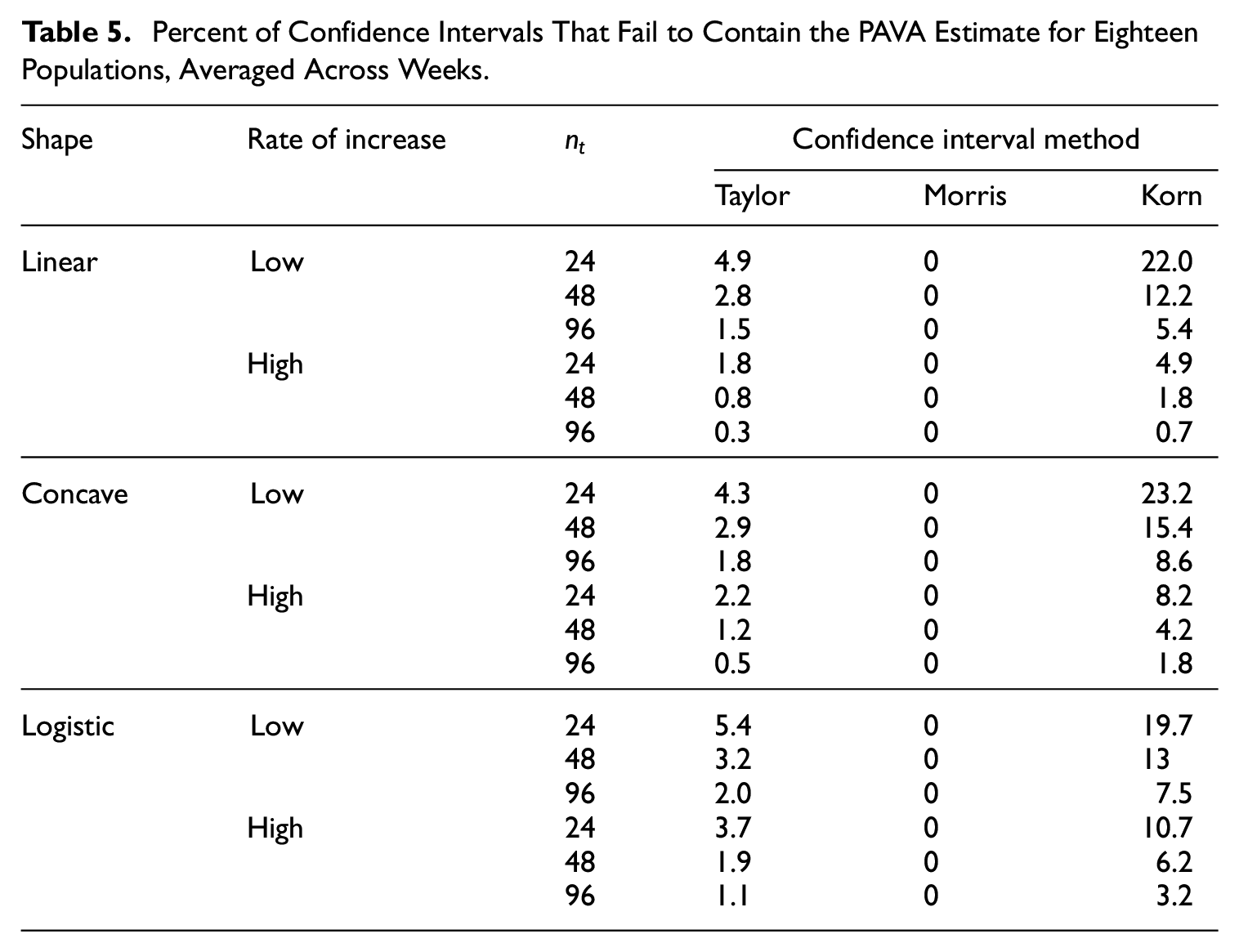
Table 5 summarizes the percent of intervals that fail to include the PAVA estimate (
Percent of Confidence Intervals That Fail to Contain the PAVA Estimate for Eighteen Populations, Averaged Across Weeks.
4. Discussion
We considered the problem of estimating a time series of population means from a series of sample surveys when the means are known to be nondecreasing. We introduced the standard survey estimators of the series of means, which are not guaranteed to be nondecreasing. We employed the Pool Adjacent Violators Algorithm (PAVA) to turn the series of standard survey estimates into a nondecreasing series.
The paper focuses on inference for the nondecreasing series. A Monte Carlo simulation was conducted to evaluate the performance of five interval estimation methods: normal-theory intervals based on the standard survey point estimator of the mean and the Taylor series estimator of its variance; normal-theory intervals based on the nondecreasing PAVA estimator of the mean and a unique jackknife estimator of its variance developed here (jackknife-
The results showed that the jackknife-
Because jackknife intervals are centered around the monotonic estimate, they are guaranteed to contain that estimate. Taylor and Korn intervals are not guaranteed to contain the monotonic estimate. The failure to contain diminishes in frequency with increasing sample size or increasing signal-to-noise ratio.
The standard survey estimator of the population proportion is a ratio estimator; it is known to be a consistent and nearly unbiased estimator. Because of the averaging that takes place within its algorithm, the sum of the PAVA estimators over all times within the estimation window (
Because its Monte Carlo coverage probabilities approached the nominal value of 95%, its half-widths were narrow relative to intervals from the other approaches, and its guarantee of containing the monotonic estimates, we can recommend in many applications the use of the jackknife-
Choosing the degrees of freedom for the jackknife-
Finally, our results and recommendations are subject to various limitations. The jackknife intervals rely on asymptotic normal theory; thus, for inferences on population proportions with small sample sizes or with the target proportion near 0 or 1, the symmetric interval estimation methods developed here may perform poorly. The Monte Carlo study only included eighteen populations defined by the shape of the series of population proportions, the rate of increase of the series, and the sample size per weekly time period. It only included time series of length 24. Within each of the 24 time periods, we generated the survey data for the simulations using the simplest possible sampling design: simple random sampling with replacement. Results of the simulations may have been different under alternative population assumptions or series lengths.
Results may also have been different under alternative sample designs. Before relying too heavily on the jackknife methods, it would be useful for future users to conduct additional Monte Carlo work to verify both the performance of the jackknife method and the choice of degrees of freedom under complex sampling designs.
Footnotes
Acknowledgements
The authors thank NORC at the University of Chicago for funding the work of this article. The jackknife method studied here was initially conceived while conducting work on the National Immunization Survey, sponsored by the Centers for Disease Control and Prevention. The authors are grateful to James A. Singleton (National Center for Immunization and Respiratory Diseases, Centers for Disease Control and Prevention) for suggesting the topic of nondecreasing estimation during the time of the COVID-19 pandemic. Finally, the authors would like to thank the referee and the associate editor for suggesting the
Funding
The author(s) disclosed receipt of the following financial support for the research, authorship, and/or publication of this article: The author(s) received financial support from NORC at the University of Chicago for the research, authorship, and/or publication of this article.
Received: September 2023
Accepted: September 2024