
Abstract
Rising nonresponse and the increasing costs of conducting surveys are creating pressure on survey organizations to efficiently allocate resources. The challenge is to produce the highest quality data possible within a fixed budget. We use a stopping rule designed to minimize a function of cost and errors. The rule is based on the product of predicted costs and the predicted mean squared error of a survey estimate. We simulate the impact of implementing the stopping rule on the 2019 US Survey of Doctorate Recipients (SDR), which is a longitudinal survey conducted every two years in the US using web, mail, and CATI. We vary the types of models used to generate the input predictions (parametric regression vs. nonparametric tree models) and the timing of the implementation of the rule. We found that the modeling approach made less difference, while the timing of the implementation of the stopping rule made a large difference in outcomes. The rule is multivariate and optimizes outcomes for two variables. It performed better for one variable, leading to reduced costs and only small increases in errors. The other variable had larger error increases.
1. Introduction
Adaptive Survey Design (ASD) seeks either to maximize data quality for a fixed budget, or to meet a specified quality standard while minimizing cost through a set of pre-specified design protocols. These protocols are developed prior to data collection using existing data, including the results of experiments (Schouten et al. 2017). ASD strategies generally succeed by allocating effort across the sample differentially—applying relatively more effort to some cases and less effort to others. This can be accomplished in a number of different ways. Some studies assign different modes to different subgroups, with high-cost but high response rate modes assigned to low-responding groups, and low-cost but low response rate modes assigned to high-responding groups (Calinescu et al. 2013; Lynn 2013; Mitchell et al. 2014). Other studies prioritize cases that are judged to be important, for example, subgroups with relatively low response rates (Calinescu and Schouten 2016; Lynn 2013; McCarthy et al. 2017; Wagner et al. 2012). While the goal is higher response rates for the prioritized groups, this comes at the cost of increased effort. Previous implementations of ASD have allocated effort based on whether cases were underrepresented (i.e., increasing effort on these cases) or overrepresented (i.e., decreasing effort on these cases; Coffey, Reist, and Miller 2020). Other studies have used stopping rules to divert effort from cases that are not expected to contribute to estimates (Lewis 2017, 2019; Rao et al. 2008; Wagner and Raghunathan 2010). However, these stopping rules have focused on quality and have not explicitly incorporated the cost dimension. A recently proposed stopping rule attempts to address this gap by explicitly including both costs and quality as components of a stopping rule (Wagner et al. 2023). Among these rules, only the rule proposed by Lewis (2019) can accommodate optimizing across multiple estimates.
Responsive survey design (RSD) is another approach where survey designs are changed based on data from the field. RSD structures data collection as a series of phases, where each phase is complementary to previous phases such that biases are reduced by each subsequent phase. RSD uses data from the active data collection to decide when to terminate a protocol using a concept called “phase capacity” (Groves and Heeringa 2006). In the RSD context, when a particular set of design features, that is, a “phase,” is no longer leading to changes in estimates, then that phase has met its capacity. At that point, a new set of design features should be implemented with the goal of addressing any biases resulting from the previous phase(s). A stopping rule could be seen as a specific instance of phase capacity where the next phase is no further effort.
However, the efficiency of stopping rules may be limited if inputs to a stopping rule, namely the predictions about costs and quality (i.e., bias or mean squared error), are inaccurate. For example, if an inexpensive case is inaccurately predicted to be costly and, therefore, is stopped, then a potential complete case would have been forfeited. Several recent publications have compared different approaches to making these predictions. Several of these papers contrast Bayesian approaches, using prior information from historical data or other sources, with maximum likelihood methods and no prior information (Coffey, West, et al. 2020; Schouten et al. 2018; Wagner et al. 2020; West et al. 2021). By incorporating information from experts, literature, and historical data into a Bayesian prediction model, these approaches aimed to improve the performance of decision rules based on these predictions.
In the current paper, we present the results of a simulation study that introduces a new multivariate version of the rule proposed by Wagner et al. (2023). The simulation study also explores the impact of two key components of the stopping not studied in the Wagner et al. (2023) experiment: (1) the modeling approach (parametric vs. nonparametric) used to generate predictions that serve as inputs to the rule, and (2) the timing of the implementation of the rule. The inputs to the rule are predictions for both costs and quality generated by both parametric regression models and nonparametric tree-based models. This study compares those two approaches as well as a third hybrid approach that uses the model with empirically-demonstrated better performance. We also examine the timing of implementation of the rule as this may also influence the rule performance. Collectively, these results provide innovative extensions of an existing stopping rule.
2. Background
Declining response rates are one of the key challenges currently confronting surveys (Curtin et al. 2005; Luiten et al. 2020; Williams and Brick 2018). To address this challenge, new survey designs have emerged that aim to control costs while ensuring high-quality data collection. Advances in survey technologies, specifically computerized survey management, have allowed for more frequent (even continual) review of case management. The constantly updated data from the field provides the critical information needed to implement ASD and RSD decision rules.
One type of decision rule is a stopping rule, where case managers decide to stop spending time and money on sampled units who, at the time of rule implementation, are deemed unlikely to change estimates or may be expensive to recruit. These rules stop attempts on all cases for which the decision rule criteria are met. Current proposed stopping rules for surveys are focused on the quality dimension (Lewis 2017, 2019; Rao et al. 2008; Wagner and Raghunathan 2010) and implicitly assume that all active cases have the same cost. Rao, Glickman, and Glynn (2008; RGG), for example, developed a rule that ceases to collect additional waves in a mailed survey once the latest wave does not change estimates relative to those derived from a previous wave. RGG included imputation of values for nonresponding cases as a part of the evaluation. Lewis (2017) developed a rule based on RGG that uses weights, rather than imputation, to account for nonrespondents. Lewis (2019) extended the approach by looking at a multivariate version of the earlier rule. Wagner and Raghunathan (2010) adopted a similar approach based on the probability of increasing the quality of estimates resulting from an additional wave.
Another feature of stopping rules that has not been explicitly considered before is the optimal timing of the implementation of the rule. The question is not relevant for stopping rules that stop all cases at the same time, but concerns when to stop a subset of cases. In practice, this can be implemented at different or even multiple points in time. There is a tradeoff that should be considered when determining whether to implement such a stopping rule earlier or later in the field period. When implemented earlier, the possibility of cost savings is improved by preventing attempts being made on cases that likely would be stopped. However, if implemented later, there are more data available from the current wave and set of cases to aid in improved predictions.
In addition to the timing of the decision, the quality of the inputs to decision rules plays a role in determining their effectiveness. In the past, responsive survey designs have produced uneven results (Tourangeau et al. 2017). One possible explanation might be that the rules that are used to trigger the time to end one phase and to move to the next phase are not sufficiently precise. Imprecision in the inputs or the rules themselves might lead to inefficiencies that reduce the overall effectiveness of the RSD. For example, an effective phase may be stopped too early or, conversely, a phase may be allowed to go too long, which can result in the inefficient use of valuable resources on an ineffective protocol.
Parametric models are commonly-used tools to create these inputs (Peytchev et al. 2022; West et al. 2021; Wu et al. 2022). Recent research has focused on how these methods could be improved by using Bayesian methods to incorporate historical data, expert opinion, or literature reviews into a model that also uses data from the current field period (Coffey, West, et al. 2020; Schouten et al. 2018; West et al. 2021). Nonparametric approaches have been less frequently used to develop inputs to decision rules in RSD (Wagner et al. 2020). Given that nonparametric machine learning approaches are designed to create predictions with low error rates, these methods may be useful. Nonparametric machine learning algorithms, in particular tree-based approaches, may be useful when the functional form of the underlying model is not well understood (Kern et al. 2019).
In an effort to improve upon the existing research on stopping rules, we use a simulation study to examine whether a stopping rule, including predictions about costs and errors as inputs, can lead to improvements in cost-error tradeoffs (e.g., a large reduction in costs with small increases in errors or reductions in error for equal costs). This rule builds upon prior research in this area (Coffey and Elliott 2023), which found that implementing a stopping rule based on predictions of costs and errors lowered costs substantially but led to minor increases in the standard errors of estimates. Wagner et al. (2023) have also found that implementing a stopping rule based on inputs generated from Bayesian models did not lower costs but led to an increase in the quality of the estimates. Wagner et al. (2023) also applied a multivariate implementation of a univariate decision rule. That is, they implemented the univariate rule on multiple variables. Cases were stopped if any univariate rule indicated that they should be stopped. The research presented improves on these findings by simulating the use of inputs generated in two different ways in a critical design decision—a case-level stopping rule. This simulation also varies the timing of the implementation of the rule.
3. Data and Methods
3.1. Data
The data used in this study come from the 2019 Survey of Doctoral Recipients (SDR). The SDR, sponsored by the National Center for Science and Engineering Statistics (NCSES) within the National Science Foundation (NSF), is a biennial longitudinal survey that measures the characteristics of doctoral recipients from a sample of all research doctorates earned in the US. New samples are drawn each wave from the Survey of Earned Doctorates (SED), which is an annual near-census of all newly earned research doctorates. The survey is multimodal, conducted using web, mail, and CATI. Refusals are re-approached as a part of the protocol. Overall, the 2019 SDR included 80,882 individuals who responded to the survey out of 119,473 eligible persons, with a weighted response rate of 69% (NCSES 2021). The SDR has three separate cohorts: (1) a continuing cohort (those who have completed an interview in a previous wave), (2) a new cohort (recent PhDs who have been sampled for inclusion in the SDR), and (3) a supplemental cohort of existing PhDs who have not been previously interviewed. This analysis focuses on the continuing cohort, which includes a large majority (95,414/119,473 = 79.9%) of all sampled cases and has data from a previous interview for the prediction models. Of these 95,414 continuing cohort members, 67,428 completed the 2019 survey and also responded in 2017. We have also carried out the analyses for the other two cohorts; these results are included in Appendix D and are very similar to those of the continuing cohort.
The previous data come from the 2017 SDR. The 2017 SDR data are available for all continuing respondents to the survey. Additional data come from the Survey of Earned Doctorates-Doctorate Records File (SED-DRF) which contains a list of every person who received a doctoral degree and is updated annually after completion of the SED. We used fourteen variables from the SED-DRF as predictors in the models for the new and supplemental cohorts. The outcome variables for our simulation models are two key variables from the survey: (1) an indicator variable of whether the person is employed by an educational institution [EMED], and (2) current annual salary [SALARY]. We deem these variables as “key” because they are frequently used among the scientific products we reviewed (Ong et al. 2022) and important to NCSES’ reporting. EMED and SALARY are available in both the 2017 and 2019 files. The predictor variables from the 2017 SDR and SED-DRF are described in more detail in Appendix A.
The 2019 SDR Paradata file contains attempt-level data for each individual. These records include, for each contact attempt, the following variables: a “task order” that records the temporal ordering of each attempt, the mode of contact (web, mail, or CATI), the date and time of the attempt, the survey completion mode (if applicable for an attempt: web, mail, CATI), and an outcome code (e.g., “complete”). One row corresponds to one contact attempt, so an individual may have multiple rows of records if the individual was attempted more than once. Overall, the 2019 Paradata file has 1,097,687 records of attempts for 119,473 unique individuals contacted in the sample. The Paradata file is used to estimate attempt-level probabilities of response which are used in our simulation study. The variables from the Paradata file that were used to make predictions are also listed in Appendix A.
We considered the contact attempt with the most recent date preceding the date of completion as the contact attempt resulting in the survey completion. For example, if the most recent attempt on a case was an email that was sent on June 8th and the survey was completed on June 9th, we assume the email was the attempt that resulted in completion. If multiple contact attempts were made on the day that is the closest to the date of completion, we selected the last contact attempt as the contact attempt resulting in the survey completion. Attempts made after survey completion were excluded.
Missing data rates are high for some of the variables used in this analysis that are found in the SED-DRF, including marital status, number of dependents, post doctorate employment, estimated salary, and post doctorate plans. This could be caused by multiple factors, such as changes in the SED questionnaire over time leading to different variables measuring similar concepts (e.g., expected income), or some variables being measured through different branching that causes participants to not answer some questions, for example, a new cohort respondent may not have had a job at the time of completing the survey. In order to avoid large numbers of observations being deleted, we treated missingness as a “valid” category for these variables. The variables from the SED-DRF were used for the new and supplementary cohorts. Levels of missing data, therefore, were lower for the continuing cohort as all cases used in the analysis had been interviewed in 2017.
3.2. Methods
In this section, we first describe our proposed stopping rule. We then describe the model selection procedures for the models used to generate inputs to the stopping rule. Finally, we describe the design of the simulation study.
3.2.1. Proposed Stopping Rule
The proposed stopping rule minimizes the product of cost and mean squared error terms. This function allows for proportional changes in either costs or MSE to have equal weight in the optimization. Certainly, other functions are possible. Coffey and Elliott (2023), for example, use the ratios of both the RMSE and costs under different strategies for optimization. It is also possible to choose functions that put more weight on one or the other term. In our approach, both costs and the survey data are predicted. The rule is based upon that implemented by Wagner et al. (2023).
We use the following notation. At a given point in time, there are

The first estimate on the right-hand side of the equation can be defined using the formula:

where the first term on the right-hand side represents the costs for currently interviewed cases (where
The error term is:
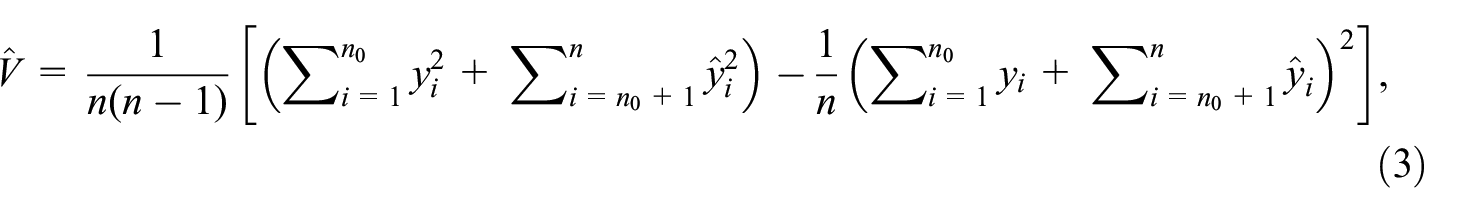
where
We assume a reasonable model for Y given available covariates to generate predicted values and treat the estimator of the total using all of the available data (including the predicted values) as unbiased. In this case, we have selected two key survey variables (Y): salary (continuous) and whether the respondent is employed by an educational institution (binary). For continuing panel members, we use data from the prior wave (2017)—including previous versions of the same measurement as well as demographic variables—to predict the current wave (2019) survey variables.
In the following, we introduce notation for identifying a subset of cases to be stopped. In order to avoid confusion, we index the cases to be stopped using the subscript notation
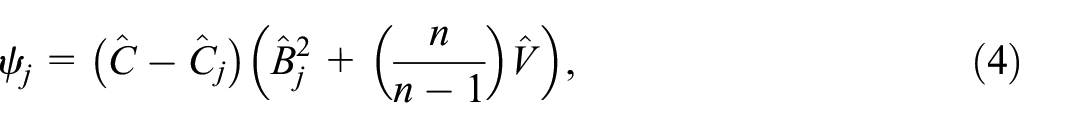
where the squared bias term is
We propose to select the case j from among the
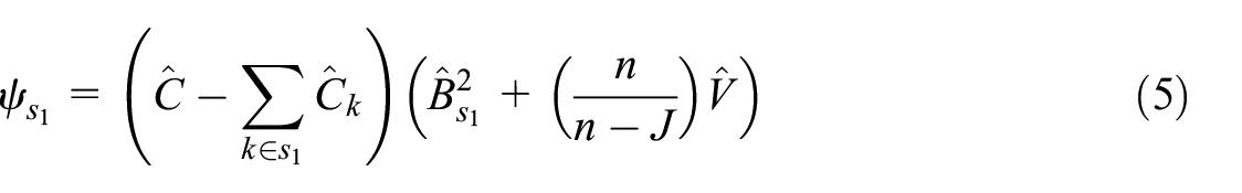
We use the
The rule defined above is designed for a single estimate. We can extend this rule to include multiple variables by taking the average of
In order to implement this stopping rule, we need predicted values of the survey variables and survey costs. In the next section, we discuss our approach to estimating costs for each of the modes of attempted contact, and then the methods we used to predict the survey variables.
Here, we note that the inputs for the three variables (attempt- and case-level costs, salary, and employed by an educational institution) could be, and are, generated in three ways: (1) using parametric regression models for all three variables; (2) using nonparametric tree-based models for all three variables; and (3) using the model with the better performance for each of the three variables. The latter approach, labeled “hybrid,” could include both parametric and nonparametric models depending upon their performance metrics.
For this simulation, we implemented the rule at a single point in time. Wagner et al. (2023) implemented the rule at multiple points in time. Optimization of such a multiple-step approach is particularly difficult. Further, there are fewer opportunities to implement the stopping rule on the SDR since it has many fewer contacts than the study that included the experiment in Wagner et al. (2023). One challenging aspect of the decision rule is the timing of implementation. The earlier it is implemented, the more cost savings that a survey would be able to gain from the implementation. On the other hand, implementing it relatively late in the process would allow for the inclusion of more information from the current wave in the estimation of our models. Therefore, we test stopping at different time points—after the third, fourth, fifth, and sixth attempts. We note that in practice, these attempt numbers will not line up at the same point in calendar time.
3.2.2. Cost Prediction
The prediction models are focused on variable costs associated with attempts to recruit panel members. These are the costs—as opposed to fixed costs—that a stopping rule can address. Attempt-level cost estimates are difficult to define for several reasons. First, costs may vary across data collection organizations. For example, larger organizations may obtain economies of scale that are unavailable to smaller organizations. Further, the costs of interviewer-administered attempts are not always directly measured. That is, interviewers report total hours worked but not hours worked on each attempt. Since the specific costs of the attempts reported in the 2019 paradata file are not available, we consulted previous research in order to establish reasonable cost estimates for attempts made in each mode.
In the paradata file, there are three modes of contact: (1) web, (2) mail, and (3) CATI. We propose methods for estimating the costs of attempts made in each mode. For the purposes of our simulation study, it is only important that the relative costs of attempts across the different modes be accurately captured.
3.2.2.1. Web
Web-based survey implementation is the least expensive mode. However, there is still a cost associated with email management tasks. There are costs to prepare the email message and the list of email addresses, as well as sending out those messages. Unlike the other modes, these costs are largely not a function of sample size. Lacking any information about the implementation of surveys using email, we assume that an email costs about 10% of a mailed survey request, that is, USD 0.18.
3.2.2.2. Mail
The cost per unit of sending surveys via mail can vary with the volume of units mailed, with larger volume leading to per unit savings. The Paradata file enables the count of the total number of mailings used in the 2019 SDR. We assume that each mailing includes a paper questionnaire, a brochure, an introductory letter, and other relevant survey materials. Grubert (2017) reported that the cost of sending a survey via mail is about USD 1.84 per mailed unit for surveys with at least 10,000 mail pieces with details about bulk mail rates included in the description. We use USD 1.84/mailing as the cost of sending the SDR via mail since the survey uses more mailings than that threshold.
3.2.2.3. CATI
We know from prior research that telephone attempts vary in length. We propose to treat attempts that result in an interview as taking longer than attempts that do not result in an interview. However, there is variation in the length of the subset of telephone attempts that do not result in an interview. The differences in length are related to factors such as whether there is contact with the respondent, whether that person refuses to participate, if an appointment is set, or any other types of results for the attempt. We ignore this variation and treat all attempts that do not result in an interview as having an average cost that is smaller than the cost of completing an interview.
The SDR takes eighteen minutes on the web (median time). CATI completion time is likely longer. We assume it takes twenty-four minutes for survey administration and six minutes for reviewing call history, phone dialing, and survey introduction. Therefore, we also assume it takes 30 (6 + 24) minutes for completed interviews over the phone and 10 (6 + 4) minutes for calls that do not result in survey completion. We assume USD 35 as the hourly interviewer wage, including employer-paid taxes and any benefits like paid time off. Under this rate, a ten-minute attempt (no interview) would cost USD 35/6 = USD 5.83, and a thirty-minute attempt (interview completed) would cost USD 17.50.
Using the predicted probabilities of response (described in the next section) and the expected costs described earlier, we can calculate an expected cost for each case. First, the expected cost of an attempt is the probability of an interview on that attempt multiplied by the cost of an interview, plus one minus the probability of an interview, times the cost of an attempt that is not an interview. In order to extend these expected costs multiple attempts into the future, we use a similar probability-based approach. The probability of surviving to attempt t for case i (i.e., not being interviewed before time
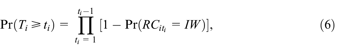
where
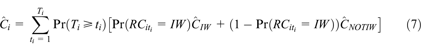
As an illustration, the expected costs for a case with
Predicting Costs for a Hypothetical Case.
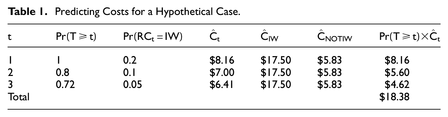
In this example, the probability of an interview on the first attempt is 0.2. Therefore, the expected cost of the first attempt is 0.2 × USD 17.50 + 0.8 × USD 5.83 = USD 8.16. The probability of a second attempt being necessary is 0.8. The cost of the second attempt is 0.1 × USD 17.50 + 0.9 × USD 5.83 = USD 7.00. Given that there is a 20% chance that this attempt will not occur, the expected cost of the second attempt is USD 7.00 × 0.8 = USD 5.60. We carry these calculations through a specified maximum of three attempts (not the maximum used in our simulation, but just for simplicity of demonstration) and sum the expected costs to USD 18.38.
3.2.3. Survey Variable and Response Propensity Prediction
We need predictions of three variables in order to implement the stopping rule:
salary (continuous),
employed by an educational institution (binary), and
attempt-level probabilities of completing an interview.
For both the survey variable and response propensity predictions, we apply two types of approaches: parametric modeling and nonparametric machine learning methods. In this section, we describe the steps used in selecting models and creating predictions from the final models.
We split the data sets into a training set and a testing set, using 75% of sample units in the 2019 SDR (n = 50,552) to train the models and the remaining 25% (n = 16,786) of the cases to test the resulting models, including using the test data for the simulation study. Item missingness on predictors led to some further loss of sample as noted in the results. This approach does allow us to test the accuracy of predictions. However, in practice, we would train models on a prior wave’s data (e.g., using 2015 data to predict 2017 outcomes as the training set), and then use the resulting trained model to predict the 2019 outcomes.
3.2.3.1. Predicted survey variables
For the parametric approach, we use a linear regression model for salary, and a logistic regression model for employment at an educational institution. The models were selected using standard regression model selection procedures, including the use of model fit statistics such as the AIC. Standard diagnostic techniques, such as examination of residuals, were also used. The predictors selected for each of the parametric models are listed in Appendix E. The nonparametric approach evaluated four different nonparametric algorithms: classification trees, random forests, neural networks, and extreme gradient boosting, and selected the one with the best performance. These nonparametric models incorporate variable selection into the model building process, so we included all available predictors. A list of variables used as predictors is provided in Appendix A. Hyperparameters for these models were tuned using five-fold cross validation with the corresponding performance metric described below.
Once the training models were established, a predicted salary or employment probability was calculated for every case in the testing set. Performance was measured using area under the ROC curve (AUC) and precision-recall area under the curve (PRAUC) metrics for response propensity and for employment at an educational institution. Root mean squared error (RMSE) was the performance measure used for salary. For the hybrid approach, we compared the performance of the parametric and nonparametric models, and selected the predicted values generated by the model with better performance (based on AUC for binary outcomes and RMSE for the continuous outcome) for each of the three variables.
3.2.3.2. Predicted probabilities of attempt-level outcomes
We know that “completed interview” and “not completed” outcomes are not equally likely, nor are the probabilities of those outcomes consistent over attempts. Therefore, we predict the response propensity at each attempt using two methods: (1) a parametric discrete-time hazard model, and (2) a tree-based nonparametric approach. The model selection techniques followed the same approach as that outlined for the prediction of the survey variables.
In the 2019 SDR, three modes of interviewing were deployed sequentially—web, mail, and CATI. There were some deviations from this sequence due to missing contact information (e.g., no street address available, therefore, after web go directly to CATI) or requests from respondents for specific modes (e.g., a respondent called the data collector and requested a mail survey before the web mode contact attempts were fully implemented). The data and simulation are based on the 2019 paradata file and, therefore, include these anomalous cases.
The modes of contact attempts (web, mail, CATI) are indicated for each case in the 2019 SDR Paradata file. We created an attempt-level file using the task-order variable found in the 2019 SDR paradata file. This allowed us to know the exact order of contact attempts per individual as well as the mode of each contact attempt. This file was used to estimate discrete time hazard models for each of the sequentially applied modes of interview. Any attempts made after initial resistance were included in these models.
In addition to variables from the 2017 SDR, we used the following variables from the 2019 SDR paradata file:
Task Order: This variable is used to determine the order of the contact attempts.
Mode: Mode used for contact attempt
Count of mode attempts: Number of attempts made in different modes to contact an individual at the time of the current attempt.
3.2.4. Simulation Study Design
The models predicting the survey variables and the response probabilities yielded the complete set of inputs required to implement the decision rule described earlier. We then simulated the impact of the decision rule on the quality of the final estimates and the final costs of the data collection. We considered three approaches:
Using parametric model inputs only;
Using nonparametric model inputs only; and
Using model inputs from the model with better performance (i.e., models with smaller RMSE for continuous variables, and models with higher AUC for binary variables), irrespective of whether the models are parametric or nonparametric.
For the simulation, we used the 2019 paradata file and deleted the actual outcome (complete or not) from each attempt. Then we use the response propensity models described earlier to create a predicted probability of responding at that attempt. The predicted probabilities from the parametric models were used as the “true” propensity for the simulation using inputs from the parametric models. The predicted probabilities from the nonparametric models were used as the true propensity for the simulation using inputs from the nonparametric models. Random draws from a uniform distribution were compared to the predicted probabilities. If the draw was less than the predicted probability, the attempt was marked as “complete” and no further attempts were simulated.
The simulation includes respondents and final nonrespondents from the 2019 SDR. Since we do not have the 2019 survey data for nonrespondents, our evaluation metrics rely on the predicted survey variables, which are available for the full sample. We have predictions for nonrespondents and, therefore, we can include them in the simulation. Excluding them would have negative consequences since they are likely to be more costly and may have predicted values with means that are different from those of respondents. For each simulation, we use the actual sequence of attempts and this sequence was allowed to continue up to the last attempt that was actually made. As a result, the simulated results of when to stop always lead to fewer attempts than occurred in the actual 2019 SDR data collection.
We also had the predicted survey values for all cases in the testing set including nonrespondents (excluding the cases with missing data on predictor variables). We used these predicted survey values, along with the predicted probabilities and fixed costs of attempts described earlier, as inputs to the rule specified in Equation (2). If a case was stopped, then it was treated as a nonrespondent (i.e., its predicted values on the survey variables were excluded from estimating the mean for respondents) and its future costs were dropped from the total cost of the survey.
Once the simulation was complete, we compared the means of the predicted values for the survey variables for the full sample (
In addition to varying the models used to create the inputs, we also varied the timing of the implementation of the rule. We simulated implementation at four different time points (after the third, fourth, fifth, and sixth attempts). In sum, we compare cost and error tradeoffs from using three different modeling approaches to generate inputs to the decision rule at four different time points, for a total of twelve simulations. Due to the large computational effort required for each of these twelve simulations, we repeated each simulation ten times to provide reliable results.
4. Results
In this section, we review the predictions made from both the parametric and nonparametric approaches for the three input variables used by the stopping rule. Then, we examine the results from the simulation study. We focus on the continuing cohort, which is the largest cohort. Results for the new and supplemental cohorts are available in Appendix D.
4.1. Prediction of Survey Outcome Variables
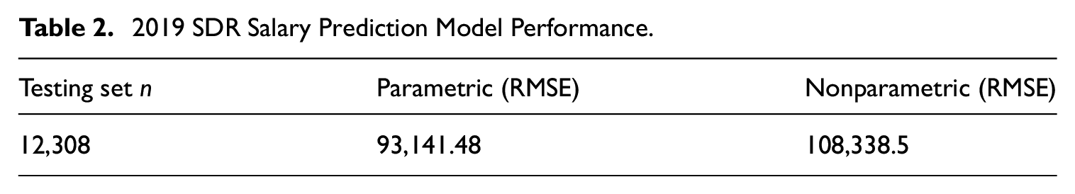
We start with the salary variable from the 2019 SDR. Table 2 shows the case-level number of observations in the testing set, and the RMSE values for the parametric and nonparametric approaches. Note that the number of observations excludes the cases with missing data on the predictor variables that were used to predict the value of salary. We find that the preferred approach was the parametric approach as the RMSEs are lower for the parametric model.
2019 SDR Salary Prediction Model Performance.
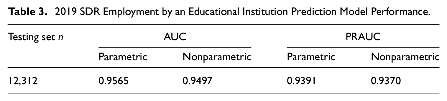
The other survey outcome variable is employment by an educational institution (EMED). Table 3 presents the model performance metrics in the form of area under the curve and precision-recall area under the curve (AUC and PRAUC). The case-level number of observations excluded the cases with missing data on predictors that were used to predict EMED. Overall, the parametric models once again performed better when compared to the nonparametric approaches, regardless of which metric was used to measure model performance, though the performance of the nonparametric model is quite close to the parametric models for both the AUC and PRAUC metrics.
2019 SDR Employment by an Educational Institution Prediction Model Performance.
4.2. Prediction of Probability of Response
Table 4 presents area under the curve (AUC and PRAUC) model fit metrics for both the parametric and nonparametric models for predicting response propensity. The number of observations is the number of attempts in the test data set after excluding the cases with missing data on predictors. The mode in each row is the mode in which the interview was completed. Each column includes only those individuals receiving at least one attempt in this mode. Therefore, the number of attempts analyzed may be less than the overall number of attempts (i.e., the “Overall” column). Looking at both the AUC and PRAUC metrics in Table 4, the nonparametric approach is better at predicting response propensity compared to the parametric approach for all scenarios.
Evaluation of Response Propensity Predictions for the 2019 SDR.
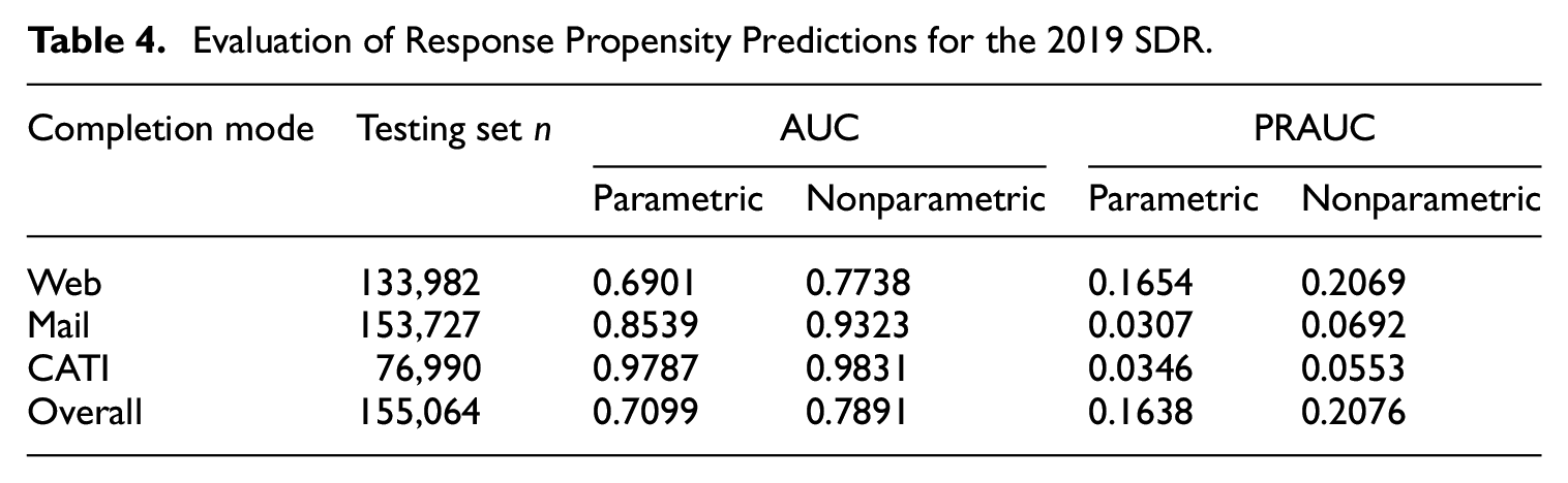
In sum, the parametric models are better at predicting the survey outcome variables and the nonparametric models are superior when predicting response probabilities. Therefore, when we apply a “hybrid” approach, we use predictions from the parametric models for the survey outcome variables and from the nonparametric models for the response probabilities in the simulation.
4.3. Simulation Study Results
Our proposed stopping rule is tested in a simulation study to assess its effectiveness in terms of cost and the impact on estimates. As with the evaluation of the predictions, in this section, we focus on the continuing cohort. Results for new and supplemental cohorts are available in Appendix D.
First, we look at the biases in point estimates and the standard errors of descriptive estimates under the three approaches. Table 5 compares the estimated mean annual salary between the full sample and the simulated set of respondents without and with the stopping rules applied. The estimates resulting from using the nonparametric approach have the lowest biases, but generally have the largest standard error estimates. Overall, the parametric approach leads to estimates that have the largest bias compared to the full sample estimate, but comparable standard error estimates to the hybrid approach. The lowest MSE (see Table 5 below) is achieved by the hybrid approach when implementing the rule at the sixth call attempt. However, the increase in MSE due to stopping is relatively small across the three approaches at this call attempt. On the other hand, the increase in MSE was relatively large across all methods for the earlier times of stopping (i.e., after the third and fourth attempts).
Continuing Cohort Mean Predicted Salary for the Full Sample, Mean Predicted Salary, Standard Errors, Estimated Biases, Count of Respondents, and MSE for Both the Simulated Respondents and Simulated Respondents After Stopping, by Modeling Approach and Attempt Prior to Implementation.
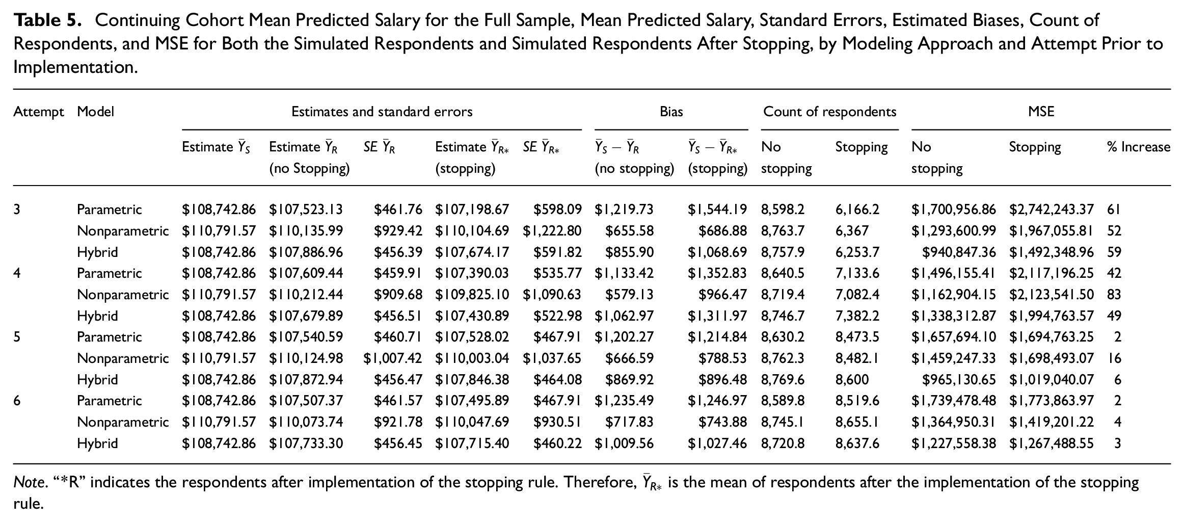
Note. “*R” indicates the respondents after implementation of the stopping rule. Therefore,
Table 6 compares estimated proportions of persons that have employment at an educational institution (EMED) in the full sample to both the simulated set of respondents and the simulated respondents following the implementation of the stopping rules. In this case, the increases in MSE are much lower across all modeling approaches and the timing of the implementation. In fact, the MSE is decreased when the rule is implemented after attempts 5 to 6 except for the parametric approach after the fifth attempt.
Continuing Cohort Proportion Predicted to Be Employed by Educational Institution for the Full Sample, Proportion Predicted to be Employed by Educational Institution, Standard Errors, Biases, Count of Respondents, and MSE for Both the Simulated Respondents and Simulated Respondents After Stopping, by Modeling Approach and Attempt Prior to Implementation.
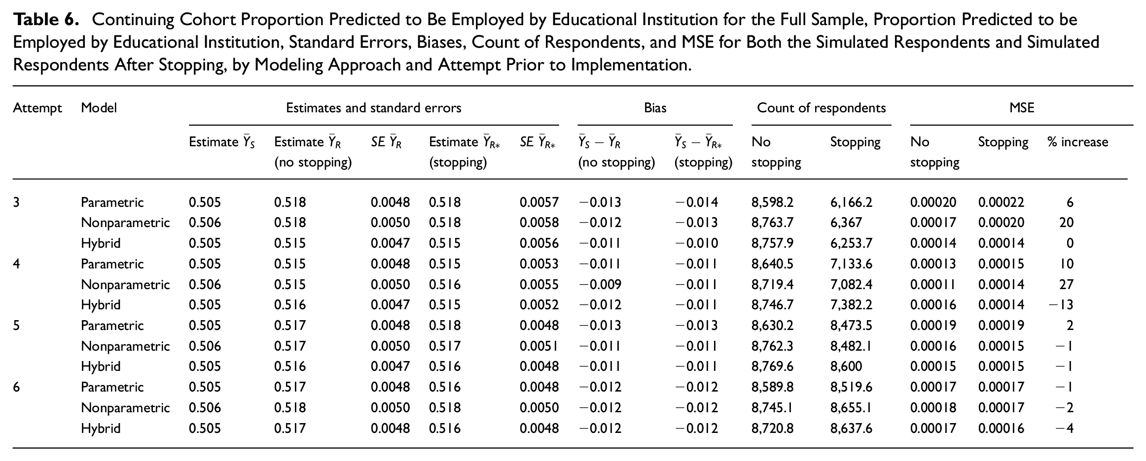
Table 7 presents information about the estimated costs of data collection for the continuing cohort, broken down by each prediction method and attempt number. The table also includes MSE per dollar and MSE times the total cost. The base cost of the full data collection for the continuing cohort ranged from about USD 136,000 to USD 144,000. This cost is the marginal cost of data collection for this cohort and is based on the methods for estimating costs described in the Methods section. In general, the timing of the rule implementation does have an impact on savings. Earlier implementation leads to greater savings. In each simulation, the stopping rule led to decreased per interview costs. These per interview savings are relatively small at later attempts (5 and 6). We also calculated “MSE per dollar” as a relative cost measure. The goal is to most efficiently use a fixed budget to produce the lowest MSE possible. For the salary variable, the stopping rule actually creates inefficiency, as indicated by the higher “MSE per dollar” ratios in Table 7. Similar inefficiency is created for the employed by educational institution variable when the stopping rule is employed, although the relative inefficiency is less for this variable.
Continuing Cohort Total Cost, Dollars per Interview, and MSE/Cost Comparisons by Estimated Mean Salary and Proportion Employed by Educational Institution.
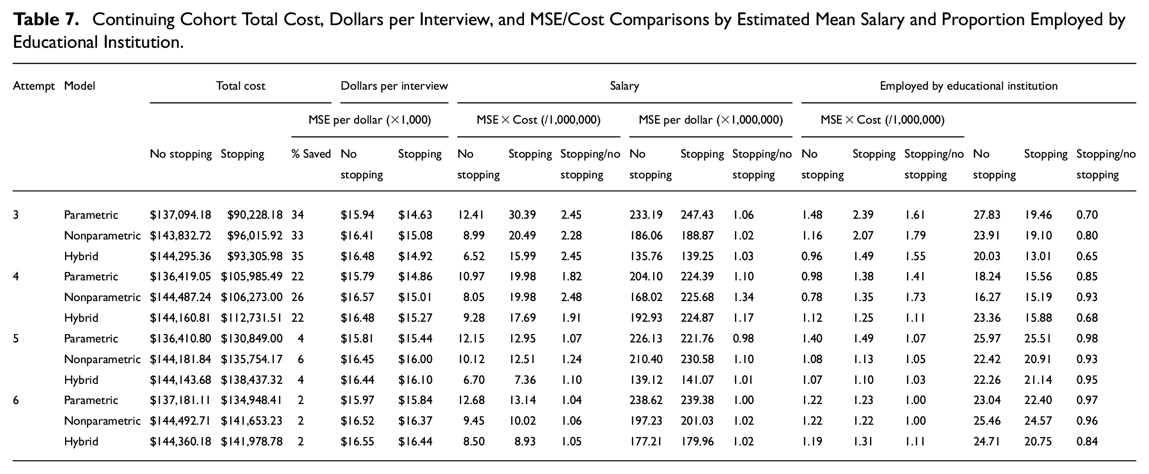
The basis of our stopping rule is the product of costs and MSE. We included that measure for each simulation and both variables in Table 7. On this measure, the rule performs better for the educational institution estimate with reductions in this quantity when the rule is implemented after the third or fourth attempts. When applied to the salary estimates, the stopping rule never achieves reductions in this quantity (costs multiplied by MSE) relative to not implementing a stopping rule. In this case, large reductions in the product of MSE and cost may be difficult to achieve for both variables.
Overall, the stopping rule is effective at achieving cost efficiency. It is less effective at controlling errors. This is particularly true with respect to the salary estimates. For the educational institution estimates, the rule proved to be more effective at balancing costs and errors. This highlights that multiple estimate objectives may require tradeoffs. We did not see big differences across the three modeling approaches, but gains with respect to costs appear to be greater when the rule is implemented earlier.
5. Summary and Conclusions
We used simulation to investigate the impact of a stopping rule on costs and errors in the SDR. The stopping rule implemented a new multivariate approach. The simulation varied two key components of the rule. First, we used two different modeling approaches (nonparametric and parametric-) to generate the predicted values used as inputs for the decision rule. We found that the parametric model better predicted our two key survey variables (salary and employment at an educational institution) and the nonparametric model performed better when predicting response propensity. Therefore, we also tried a hybrid approach that included predicted survey variables from parametric models and predicted response propensity from nonparametric models. Overall, we found that the parametric and hybrid model approaches led to increases in the MSE (sometimes rather large increases) and uniformly produced cost savings, but not cost efficiency in terms of MSE per dollar. That is, the stopping rule reduced the overall costs without increasing the level of quality (measured by MSE) produced per dollar. The nonparametric rule, on the other hand, led to similar or somewhat lower costs and much higher MSE, mainly at the early contacts. Therefore, the model fit and accuracy of predictions does seem to matter in the implementation of the rule. This is consistent with results from a recent simulation study of adaptive survey designs (Zhang 2022).
The second component of the rule that was varied was the timing of the implementation of the rule. This feature did have a strong influence on cost savings and the quality of estimates as measured by MSE.
The multivariate rule, using simple averaging across the two variables to make the stopping decision, worked better for estimates of the proportion employed by an educational institution than the estimates of the mean salary. This could be the result of the fact that the relative MSE of the salary variable is larger. It is possible that other multivariate rules (e.g., a rule that differentially weights each estimate used in the optimization) may work better. As measured by MSE per dollar, the implementation of the rule used here created relative inefficiencies across both estimates and all stopping times. On the other hand, as measured by the product of cost and MSE (the function used by the rule), the rule did produce efficiencies for the employed by an educational institution estimate. For this estimate, the rule even led to relative reductions in MSE when it was implemented after the fifth or sixth attempts. The costs, as measured on a per-interview basis, were lowered by the stopping rule. Stopping earlier led to greater cost reductions. It might be the case that other functions of cost and quality might lead to improved optimization.
Further, with respect to the differing findings across the two estimates, it might be that optimizing the results for both estimates is not feasible or that a different multivariate rule might do better. Wagner et al. (2023) implemented a univariate rule on multiple variables. As with this study, results were mixed across the eleven variables considered. Defining a rule that optimizes across multiple estimates is an open question for future research.
The approach appears to be successful in controlling costs but may not be as effective in reducing errors. However, it is worth noting that the estimates of these errors (bias and variance) are based upon prediction models and as such may not be correlated with true errors if the underlying models are misspecified (Zhang 2022). Nevertheless, balancing cost reduction with error control is crucial, especially in the current environment where funding for large surveys has remained stagnant for almost two decades, and statistical agencies are expected to accomplish more with the same budget. The stopping rule proposed in this study can be an important tool in meeting the objectives of maximizing quality for a fixed budget.
There are some limitations in this study. First, this is a simulation and the logical next step is to experimentally test our models in an actual data collection setting with a control group. Reducing effort on some cases might lead to additional effort on other cases. Our simulation approach does not allow us to test this possibility. Second, our estimated costs for each type of attempt may differ from those experienced by different data collectors. In that case, updated costs estimates would be required to re-run the simulation and determine if comparable conclusions can be drawn. Third, the multivariate rule, as implemented, led to greater success with one variable than the other. Identifying methods that control errors and costs most effectively across multiple estimates is an area for additional research (Zhang et al. 2021). Finally, the proposed stopping rule relies upon predicted point estimates and ignores the uncertainty in these predictions. New rules have been suggested that attempt to account for this uncertainty (Zhang 2023). In order to address these issues in practical situations, it would be useful to simulate results with existing data to determine how effective the approach is across multiple variables, and how sensitive the results are to different modeling approaches and available data for predictors.
The simulation study suggests that cost savings are possible while controlling the quality dimension. A reduction in the cost of the survey can be used to increase the quality in other aspects of the survey, particularly by increasing the sample size. The proposed stopping rule appears to offer a path to controlling costs with marginal increases in error. This allows statistical agencies to meet objectives in an efficient manner. This approach merits additional testing and consideration. Optimizing the outcomes for multiple estimates is a challenge that will need to be addressed as most surveys are interested in multiple outcomes.
Footnotes
Appendix A
List of Variables Used for Response Propensity Predictions.
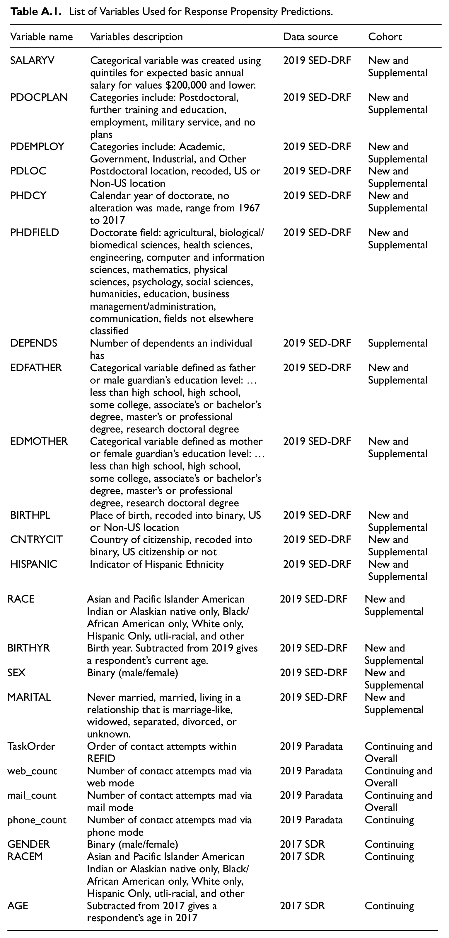
| Variable name | Variables description | Data source | Cohort |
|---|---|---|---|
| SALARYV | Categorical variable was created using quintiles for expected basic annual salary for values $200,000 and lower. | 2019 SED-DRF | New and Supplemental |
| PDOCPLAN | Categories include: Postdoctoral, further training and education, employment, military service, and no plans | 2019 SED-DRF | New and Supplemental |
| PDEMPLOY | Categories include: Academic, Government, Industrial, and Other | 2019 SED-DRF | New and Supplemental |
| PDLOC | Postdoctoral location, recoded, US or Non-US location | 2019 SED-DRF | New and Supplemental |
| PHDCY | Calendar year of doctorate, no alteration was made, range from 1967 to 2017 | 2019 SED-DRF | New and Supplemental |
| PHDFIELD | Doctorate field: agricultural, biological/biomedical sciences, health sciences, engineering, computer and information sciences, mathematics, physical sciences, psychology, social sciences, humanities, education, business management/administration, communication, fields not elsewhere classified | 2019 SED-DRF | New and Supplemental |
| DEPENDS | Number of dependents an individual has | 2019 SED-DRF | Supplemental |
| EDFATHER | Categorical variable defined as father or male guardian’s education level: … less than high school, high school, some college, associate’s or bachelor’s degree, master’s or professional degree, research doctoral degree | 2019 SED-DRF | New and Supplemental |
| EDMOTHER | Categorical variable defined as mother or female guardian’s education level: … less than high school, high school, some college, associate’s or bachelor’s degree, master’s or professional degree, research doctoral degree | 2019 SED-DRF | New and Supplemental |
| BIRTHPL | Place of birth, recoded into binary, US or Non-US location | 2019 SED-DRF | New and Supplemental |
| CNTRYCIT | Country of citizenship, recoded into binary, US citizenship or not | 2019 SED-DRF | New and Supplemental |
| HISPANIC | Indicator of Hispanic Ethnicity | 2019 SED-DRF | New and Supplemental |
| RACE | Asian and Pacific Islander American Indian or Alaskian native only, Black/African American only, White only, Hispanic Only, utli-racial, and other | 2019 SED-DRF | New and Supplemental |
| BIRTHYR | Birth year. Subtracted from 2019 gives a respondent’s current age. | 2019 SED-DRF | New and Supplemental |
| SEX | Binary (male/female) | 2019 SED-DRF | New and Supplemental |
| MARITAL | Never married, married, living in a relationship that is marriage-like, widowed, separated, divorced, or unknown. | 2019 SED-DRF | New and Supplemental |
| TaskOrder | Order of contact attempts within REFID | 2019 Paradata | Continuing and Overall |
| web_count | Number of contact attempts mad via web mode | 2019 Paradata | Continuing and Overall |
| mail_count | Number of contact attempts mad via mail mode | 2019 Paradata | Continuing and Overall |
| phone_count | Number of contact attempts mad via phone mode | 2019 Paradata | Continuing |
| GENDER | Binary (male/female) | 2017 SDR | Continuing |
| RACEM | Asian and Pacific Islander American Indian or Alaskian native only, Black/African American only, White only, Hispanic Only, utli-racial, and other | 2017 SDR | Continuing |
| AGE | Subtracted from 2017 gives a respondent’s age in 2017 | 2017 SDR | Continuing |
Appendix B
Count of Cases and Proportion of Attempts That Led to Survey Completion in the Test Data.
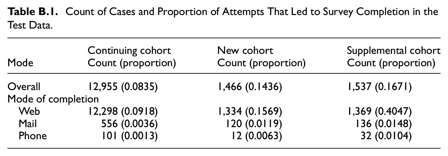
| Continuing cohort | New cohort | Supplemental cohort | |
|---|---|---|---|
| Mode | Count (proportion) | Count (proportion) | Count (proportion) |
| Overall | 12,955 (0.0835) | 1,466 (0.1436) | 1,537 (0.1671) |
| Mode of completion | |||
| Web | 12,298 (0.0918) | 1,334 (0.1569) | 1,369 (0.4047) |
| 556 (0.0036) | 120 (0.0119) | 136 (0.0148) | |
| Phone | 101 (0.0013) | 12 (0.0063) | 32 (0.0104) |
Appendix C
Appendix D
Appendix E
Funding
The author(s) disclosed receipt of the following financial support for the research, authorship, and/or publication of this article: This analysis was supported and funded by the NCSES Broad Agency Announcement research program [Contract # 49100420C0020]. The views expressed in this document are those of the authors and do not necessarily reflect the views of the National Center for Science and Engineering Statistics within the National Science Foundation.
Received: June 2023
Accepted: September 2024