
Abstract
The paper presents methodology to generate experimental small area estimates (SAE) of poverty in four West African countries: Chad, Guinea, Mali, and Niger. Due to the absence of recent census data in the four countries, household level survey data are integrated with grid-level geospatial data, which are used as covariates in model-based estimation. Leveraging geospatial data enables reporting of poverty estimates more frequently at disaggregated administrative levels and makes estimation feasible in areas for which survey data are not available. The paper leverages the availability of a recent census in Burkina Faso for evaluation purposes. Estimates obtained with the same survey instruments and candidate geospatial covariates as the other four countries are compared against estimates obtained using recent census data and an empirical best predictor under a unit level model. For Burkina Faso, estimates obtained using geospatial data are highly correlated with the census-based ones in sampled areas but moderately correlated in non-sampled areas. The results demonstrate that in the absence of recent census data, small area estimation with publicly available geospatial covariates is feasible, can lead to large efficiency improvements compared to direct estimation, and improve the timeliness of small area estimates.
Keywords
1. Introduction
This paper presents the methodology to generate experimental small area estimates (SAE) of poverty in four West African countries: Chad, Guinea, Mali, and Niger, as well as an evaluation exercise using data from another country in the region, Burkina Faso. SAE is a statistical method used to improve survey estimates by integrating survey data with geographically comprehensive auxiliary data (covariates) typically derived from census, administrative, remote sensing, or mobile phone data. Data integration is achieved with the use of statistical models to produce estimates at disaggregated geographic levels that are more accurate and precise than estimates that rely only on direct use of the survey data. More disaggregated estimates are key for a better understanding of how to target interventions for the poorest areas as well as for monitoring the impact of such interventions.
Table 1 illustrates the issues with obtaining poverty estimates at disaggregated geographic levels solely from survey data in the countries under study in this paper. The coefficient of variation estimated (cve) is a common measure used to judge the statistical precision of an estimate. Countries often adopt a maximum threshold for the mean or median cves of the estimates that can be reported, which in practice usually ranges from 0.15 to 0.3. For the countries of focus in this paper, the most recent survey estimates of poverty can be obtained from the 2018 round of the Enquête Harmonisée sur le Conditions de Vie des Ménages (EHCVM) which is available at the regional level for each country. This survey is the main output from the Harmonized Surveys on Household Living Conditions Program of the World Bank and the West Africa Economic and Monetary Union (WAEMU) Commission, which resulted in ten countries (eight WAEMU members plus Guinea and Chad) collecting household data and constructing household welfare using methodologies that were highly harmonized across all the countries and updated in line with international best practice.
Statistics of Poverty Estimates in the Focus Countries.
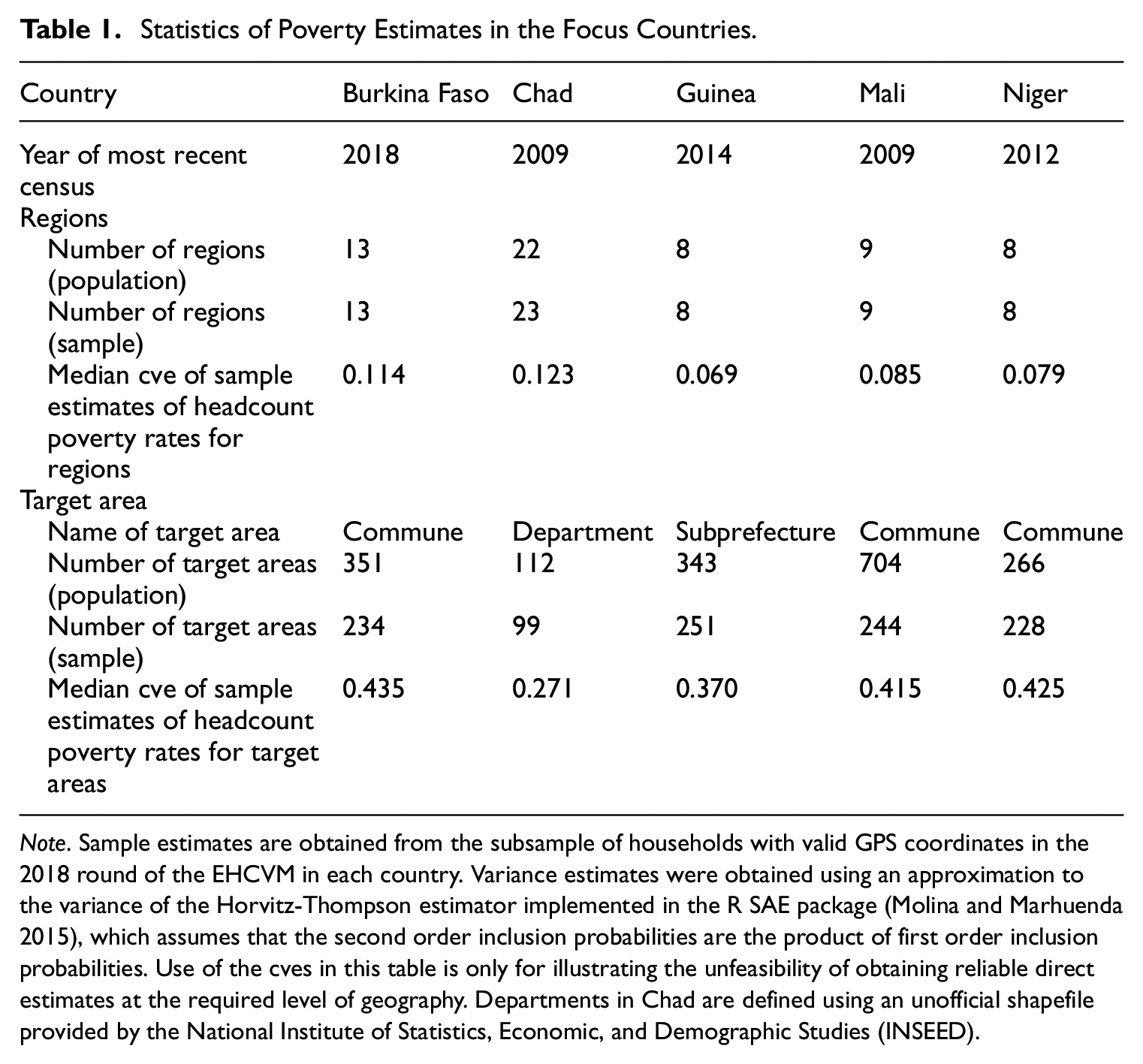
Note. Sample estimates are obtained from the subsample of households with valid GPS coordinates in the 2018 round of the EHCVM in each country. Variance estimates were obtained using an approximation to the variance of the Horvitz-Thompson estimator implemented in the R SAE package (Molina and Marhuenda 2015), which assumes that the second order inclusion probabilities are the product of first order inclusion probabilities. Use of the cves in this table is only for illustrating the unfeasibility of obtaining reliable direct estimates at the required level of geography. Departments in Chad are defined using an unofficial shapefile provided by the National Institute of Statistics, Economic, and Demographic Studies (INSEED).
Using EHCVM data, the median cve of regional direct estimates produced by the Horvitz-Thompson estimator ranges from 0.07 to 0.12, which is typically within the acceptable range for publication. However, when we examine direct estimates of the poverty rates for the set of target administrative areas, which is one or two levels below the region, the estimates are too imprecise to publish. The target geography in Chad is the latest unofficial definition of departments provided to use by the National Institute of Statistics, while in Guinea it is the Sous-prefectures, and in Mali and Niger it is Communes. At these levels, the median cve of the direct survey estimates reported in Table 1 exceeds the 0.3 threshold for each country except for Chad, where it is 0.27. In addition, not all the target areas are covered by the surveys, making direct estimation impossible for these areas. While this is the case in all countries, unsampled areas are particularly prevalent in Mali, where less than 40% of the target areas are in the sample.
Typically, small area estimation applications combine survey data with covariates from census (or other population) data. However, except for Burkina Faso, the last time a census was conducted in these countries was between 2009 and 2014. Using out-of-date census data to update small area estimates can lead to biased estimates for example, if the distribution of the census covariates used for prediction has changed over time. This is an issue that is often not discussed in applied poverty mapping work. Literature on approaches to update poverty estimates in the intercensal period includes Isidro et al. (2016), Koebe et al. (2022), and Arias-Salazar (2023). In this paper we rely on using contemporaneous geospatial covariates, as first illustrated by Battese et al. (1988; see also Nguyen 2012), to produce small area poverty estimates in countries that lack recent census data.
Advances in processing of geospatial data and the richness of geospatial data sources make their use as auxiliary information in small area models appealing. Newhouse (2024) summarizes recent literature on the use of geospatial data for small area estimation of wealth and poverty. Jean et al. (2016), Yeh et al. (2020), and Chi et al. (2022) show that satellite data are predictive of wealth indices. The present paper utilizes a method commonly used in small area estimation based on the empirical best predictor (EBP) under a nested error regression model (also referred to as mixed model; Molina and Rao 2010). When applied to predicting headcount poverty rates using geospatial covariates, this method has yielded predictions that are highly correlated with up-to-date census-based estimates in Mexico, Sri Lanka, and Tanzania (Masaki et al. 2022; Newhouse et al. 2022). The methodology we use in this paper deviates from the official approach endorsed by the World Bank’s Poverty Global Practice, as described in Corral et al. (2022), which is based on the EBP under a unit (household) level mixed model, and census micro-data as covariates (referred to as census-EBP). The main difference, besides the use of geospatial (instead of population census) covariates, is that our modeling approach utilizes only grid cell covariates, but the outcome is still modeled at the unit (household) level. This is why sometimes this latter model is referred to as the unit context model.
We explore the use of the unit context model in Chad, Guinea, Mali, and Niger that lack recent census data. We further leverage the availability of recent census data for a fifth country in West Africa, Burkina Faso, to conduct an evaluation exercise. The evaluation exercise compares estimates of headcount poverty rates obtained with a unit level model and the empirical best predictor using census covariates, with poverty rates obtained using the empirical best predictor under the unit context model with geospatial covariates.
As noted above, an alternative approach to small area estimation using geospatial covariates is to use an area level model (Fay and Herriot 1979), case in which both the direct estimates of poverty rates and the geospatial covariates are aggregated at the target area level. Hence, in the evaluation exercise presented in Section 4 we also produce estimates under a Fay-Herriot model as a way of providing additional evidence about the validity of the estimates produced under the unit context model.
Using geospatial data instead of census data in SAE and the unit context model has been criticized in recent literature (e.g., Corral et al. 2021). This is due to the possible introduction of omitted variable bias (relative to the unit level model) resulting from the aggregation of the geospatial covariates. Although a detailed discussion of this issue is beyond the scope of the current paper, being cognizant of the potential impact of using the unit context model on small area estimates is important.
First, the bias that has been reported in the literature is relative to an assumed gold-standard unit (household) level model and the availability of up-to-date household level census micro-data. It is our view that if recent census data are available, the census-EBP method should be preferred. We argue, however, that in the absence of recent census data, the use of geospatial covariates may constitute a valid alternative for providing up-to-date small area estimates until data from the next census becomes available. Second, we have observed that the extent of bias in the unit context model depends on the method used to account for sample weights. In this paper, weights are incorporated following Guadarrama et al. (2018). This weighting procedure was implemented in a way that adjusts the estimates of the regression coefficients and random effects to account for sample weights but uses the unweighted REML estimators for the variance components. As shown below, this can cause significant differences in small area estimates which are larger for models with lower predictive power, which is typically the case with unit context models. In Section 4 we explore both weighted and unweighted versions of the unit context model to assess how this impacts the estimates. Third, noting that aggregation is unavoidable due to the way geospatial data are processed, it is worth mentioning that the geographic level at which geospatial covariates are processed and linked to survey data (grid size) impacts the estimation. Because of this and because geospatial covariates can only act as proxies for the kind of variables typically used to model income (or consumption), it is reasonable to assume that the unit context model may show lower levels of predictive power and higher uncertainty than the unit (household) level model. However, because the estimators of interest are aggregations of individual level predictions, it is not obvious that the lower predictive power and higher uncertainty will substantially reduce the quality of the small area estimates obtained by using the unit context model. Finally, as is the case with any model-based method, model building, variable selection, and residual diagnostics are critical. The data analyst can try to mitigate the impact of aggregation by processing the geospatial data at the finest feasible spatial level to maximize the effective sample size. However, this may increase the risk of observing outliers in the geospatial data. The use of transformations may help make the data more consistent with the assumptions that the functional form is linear, and the error terms are distributed normally. As always, the use of model-diagnostics is crucial.
In addition, Corral et al. (2021) report concerns with the estimated measures of uncertainty under a unit context model. From our perspective, if the model assumptions are satisfied, a parametric bootstrap MSE estimator will provide a valid estimator of the uncertainty under the assumed model. Since the true data generating process is unknown, we cannot know a priori the extent to which the model assumptions are violated, regardless of the type of model assumed. In Section 4, we present results from Burkina Faso comparing coverage rates derived from the parametric bootstrap under the unit context model, treating census-based estimates as truth, with those from other estimators. For sampled areas, coverage rates under the unit context model are slightly below those from direct estimates and slightly above those obtained from an area level model, indicating that the estimated measures of uncertainty obtained through the parametric bootstrap are reasonable in this case.
In summary, we prefer to avoid making definitive statements about whether the unit context model works well or poorly. We instead posit that in the absence of a recent census, a unit context model with geospatial data may be considered as an alternative to the use of outdated census data. The presence of a recent census in Burkina Faso provides a valuable opportunity for evaluating this method. As with every SAE application, the performance of different methods will depend on the country context and the characteristics of the available survey and auxiliary data they are applied to. Evaluations of the estimates therefore remains of paramount importance.
The paper is organized as follows. Section 2 describes the data sources and the process of integrating geospatial and survey data. Section 3 presents the core of the small area methodology, model selection and assessment, small area estimation, mean squared error estimation, and measures to assess the small area estimates for all countries of focus in this paper. Section 4 presents an evaluation exercise using recent census and survey data in Burkina Faso. This allows us to compare small area estimates produced with geospatial covariates to small area estimates produced using covariate information from census micro-data. The results of the evaluation exercise add new insights to the body of literature on the use of geospatial data in small area estimation and motivate the use of the unit context model with geospatial data in the four remaining countries that lack up-to-date census data. Section 5 presents experimental point and uncertainty estimates for all countries using the unit context model. The paper concludes with a summary of the main findings and areas for further research.
2. Data Sources and Geospatial Data Integration
In this paper, we use geospatial covariates because, as shown in Table 1, the most recent censuses in the four focus countries were conducted in 2014 in Guinea, 2012 in Niger, and in 2009 in Chad and Mali. If more recent census data existed, using these data would be the preferred option. For example, several variables routinely collected in censuses such as household size, education, and sector of employment have been shown to be highly predictive of household welfare. Estimates based on recent census data are expected to be more accurate and precise than estimates based on geospatial data, which is often only available at an aggregated level (see e.g., Corral et al. 2021).
In this paper, however, we avoid using household level predictors in the model because information for the same predictors from a recent census is not available. Using old census data can be problematic because it is not guaranteed to capture developments since the last census, especially in countries impacted by rapid changes. Interpreting the estimates as if these arise from the census year requires assuming that the distribution of the census predictors, as well as their relationship to poverty, has not changed over time. This is a particular concern in countries such as these under study in this paper, which have among the highest fertility rates in the world and, in addition, have suffered from recent conflict and climate shocks which likely affected the geographic distribution of poverty and the geographic distribution of the population. Alternative sources of administrative data, such as health, land, or other administrative records, can also be useful sources of auxiliary data for small area estimation. However, these were not possible to obtain, and would not necessarily be commonly available for all four countries. We therefore decided to use publicly available, up-to-date geospatial data as covariates in small area models. The full list of candidate geospatial covariates, as well as a brief description of each of them are included in Table A1.
To estimate the model, we use survey data from the 2018 EHCVM surveys in the focus countries. The process of integrating the geospatial covariates with the survey data in each country is as follows. First, we process the covariates on a gridded shapefile with square grid cells of size 1 km2 covering the totality of the country. Then, each household in the survey is matched to a grid cell using the centroid of the Enumeration Area in which the household is located. For each country it was observed that in the 2018 EHCVM surveys, geocoordinates were not available for a small share of households (representing less than 7% of all surveyed households in all cases). We dropped these households from the data. A detailed description of the differences between the full sample and the portion with available geocoordinates that was used in the analysis is presented in Table A2.
Figure 1a and b illustrate the use of grid cells and creation of geospatial zonal statistics. Figure 1a shows the grided cells in Conakry, Guinea. Figure 1b shows the value of the average radiance of nighttime lights across grid cells in the same area. The lighter grid cells have higher values of nightlights, while the darker cells have lower values. For each grid cell, we calculated the average feature value from the raster data. In addition to these grid cell-level indicators, we also calculate mean values of the indicator at the target area level to include as predictors in small area models. Including these contextual variables at the target area level as additional covariates helps improve the predictive performance of the model.
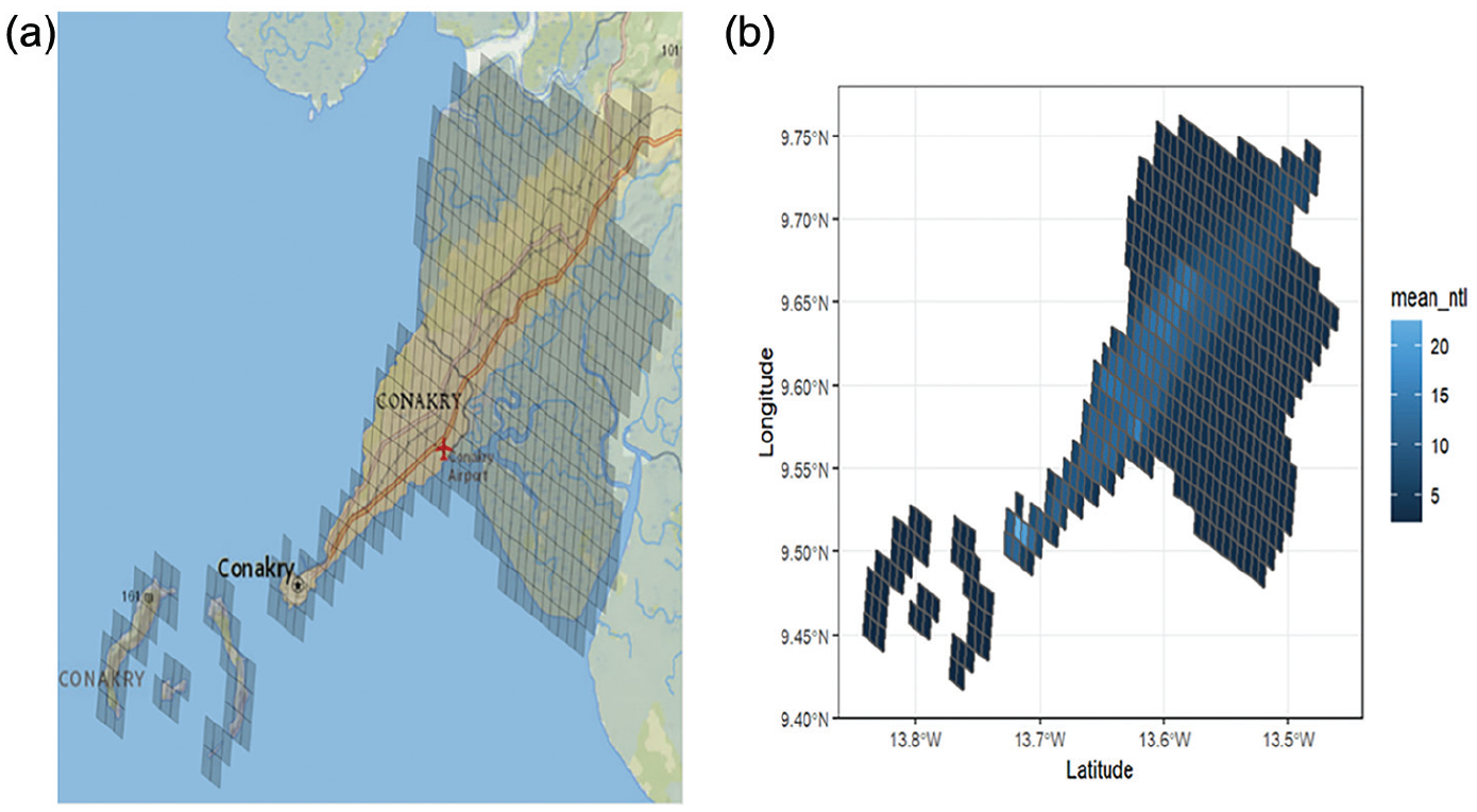
(a) Grid in Conakry, Guinea and (b) average radiance of nighttime lights in Conakry, Guinea.
3. Small Area Estimation Methodology
In this section we present a summary of the small area methodologies we use to estimate headcount poverty rates at the level of the target area in the five countries of interest. We use a version of the Empirical Best Predictor (EBP; Battese et al. 1988; Jiang and Lahiri 2006; Molina and Rao 2010; Tzavidis et al. 2018) under the unit context nested error regression model with households as the unit of analysis and covariates defined by zonal statistics of geospatial variables at grid cell level (centroid of enumeration areas within target areas). Our methodology is similar to the one used by Masaki et al. (2022), which uses small area estimation to estimate non-monetary poverty indicators in Tanzania and Sri Lanka with geospatial covariates, and Newhouse et al. (2022), which applies similar techniques with geospatial covariates to estimate monetary poverty in Mexico. Van der Weide et al. (2022) also examines the performance of poverty estimates with geospatial covariates in Malawi but using a spatial error model with sub-area level estimates of poverty rates as the outcome, and geospatial zonal statistics as covariates.
As mentioned in previous sections, when the census and survey data are collected from around the same time, using household level census covariates is generally preferred, because the census tends to contain richer auxiliary information than geospatial data. When census data are sufficiently old, however, using cluster level covariate aggregates taken from the old census can generate more accurate estimates than using old census household level covariates (Lange et al. 2021). None of these variations of covariate use, however, reflect any changes in the distribution of the census covariates since the last census. Because, except for Burkina Faso, the census data in the focus countries of this paper are not up to date, we explore the use of more current geospatial data as covariates instead of old census data.
We opt for a household level model of welfare over a grid cell level model of poverty rates because it utilizes more detailed information about the distribution of the welfare variable, and it is easier to interpret. In addition, defining the grid cell level poverty rate as the outcome to be estimated, as in the case of an area level model, requires accounting for the corresponding sampling variability, which may be challenging at such a small level of aggregation. We also prefer a household level model to an area level model because the former allows for the use of auxiliary data at the grid cell level rather than at the target area level, which can improve the accuracy and precision of the estimates, as demonstrated in Masaki et al. (2022) and Newhouse et al. (2022).
We model the household log per capita consumption as a linear function of a subset of geospatial covariates selected through Lasso. The procedure is described in detail in Appendix B. The model equation takes the form:

where
The EBP works by repeatedly simulating synthetic populations

where
In this paper we implement a version of the EBP that calculates the expected value of headcount poverty given the estimated model parameters, for each population unit (which in this case is a grid). Under the assumed linear mixed model, this expectation has a closed form. Having fit model Equation (1), the expected poverty rate for each grid is computed as follows:
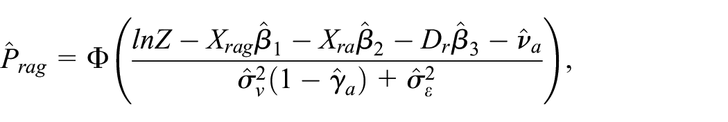
where
An alternative approach to small area estimation with geospatial covariates is modeling directly the poverty rates using an area level model (Fay and Herriot 1979). In this case, both the direct estimates of poverty rates, denoted by

where
3.1. Model Selection and Assessment
The geospatial data listed in Table A1 were used to construct averages of zonal statistics both at the grid cell level and the target area level which are used as covariates in model Equation (1). In addition, we include dummy variables at the region level. For model selection we use Lasso to select a set of predictor variables while avoiding overfitting. Estimation of the Lasso penalty parameter is implemented by minimizing the Bayesian Information Criterion (Zhang et al. 2010). The regional dummies are unpenalized and therefore are guaranteed to be selected in the model. Details are provided in Appendix B.
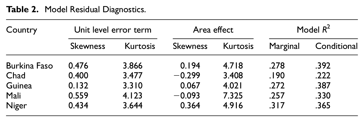
Broadly, the signs and patterns of the coefficients of the unit context model reflect a positive association between population and building density, and a negative association between welfare and remoteness, as proxied by agricultural production and a high prevalence of grassland and shrubland. Fitting model Equation (1) in the five countries under consideration leads to R2 values ranging from .19 in Chad to .32 in Niger. This range is consistent with similar applications in other contexts. In similar household level models with aggregation of geospatial covariates at similar spatial scales, the R2 was .30 in Tanzania and .27 in Sri Lanka when predicting per capita consumption, and .13 in Mexico when predicting per capita income. Geospatial variables do not vary within grids-cells and therefore can only explain variation in welfare across enumeration areas. However, the R2 is not necessarily the most accurate measure of the benefit of incorporating auxiliary data, as small area estimates based on models with weaker predictors can also be of acceptable quality. Overall, the R2 values in the focus countries indicate that the geospatial variables measured at grid cell level (enumeration areas) are moderately predictive of variation in household per capita consumption and can potentially lead to acceptable small area estimates.
Table 2 presents model residual diagnostics under model Equation (1). The error terms appear to be reasonably normal as judged from the skewness and kurtosis, though less so for the unit level error term in Mali. Figure 2 presents quantile-quantile plots for the unit and area estimated model residuals for all five countries. Overall, the results show that the log-transformed model provides a reasonable approximation to the normality of the model error terms. Additional model and residual diagnostics are presented in Appendix C.
Model Residual Diagnostics.
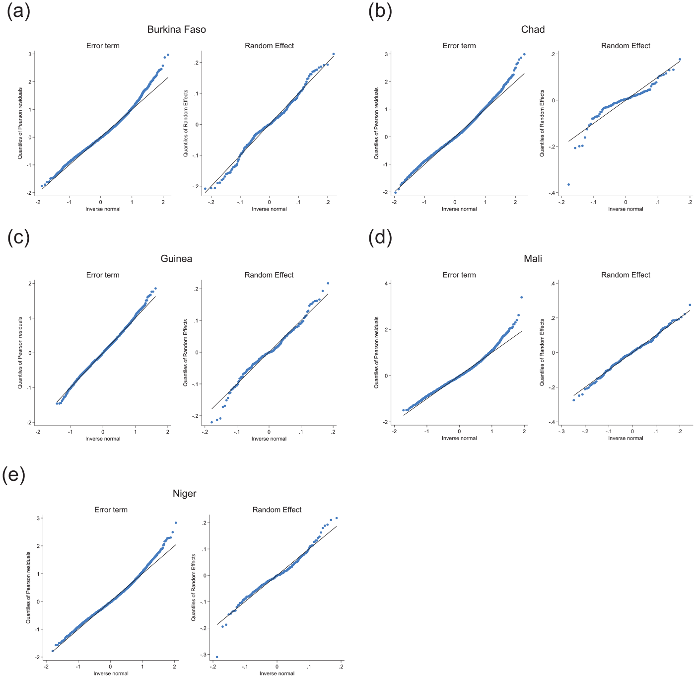
Quantile-quantile plots of unit level error terms and area random effects: (a) Burkina Faso, (b) Chad, (c) Guinea, (d) Mali, and (e) Niger.
4. Evaluation Exercise: Comparison of Geospatial and Census-Based Estimates of Headcount Poverty in Burkina Faso
Before presenting estimates of headcount poverty rates for the four focus countries that lack recent census data, we conduct a sensitivity analysis with data from Burkina Faso. The availability of a recent census in Burkina Faso creates an opportunity to assess the estimates produced with geospatial covariates and the unit context model against officially adopted EBP census-based estimates as described below.
Burkina Faso’s National Institute of Statistics and Demography carried out a census in 2018 which was utilized by the Burkina Faso poverty team of the World Bank to generate small area estimates of poverty for Communes using the EBP census methodology (Molina and Rao 2010) under a two-fold nested error regression model (Marhuenda et al. 2017). Because the census and the survey data are from a similar period, the small area estimates using census auxiliary information are considered the gold standard. Comparing the census-based estimates with estimates produced using geospatial covariates offers an appropriate testing ground for assessing the extent of discrepancies between census-based and geospatial-based estimates. This framework can also be used to compare the estimates produced by different models.
For the purposes of the evaluation exercise, we treat the census-based EBP estimates as the gold standard. The census-based estimates are compared to: (a) small area estimates under both survey weighted and unweighted versions of model Equation (1) with the outcome defined at household level and the geospatial covariates defined at grid cell level; (b) small area estimates under an area level (Fay-Herriot) model, with geospatial covariates aggregated at the target area level; and (c) small area estimates under a grid cell level model where both the outcome and the geospatial covariates are defined at grid cell level. It is important to note that the survey data was collected from the same harmonized survey instrument as the survey data for the other four countries we consider in this paper.
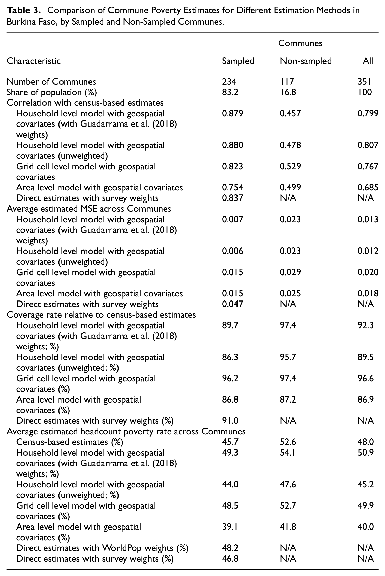
Figure 3 and Table 3 summarize the results of these comparisons. Across all Communes in Burkina Faso, we find a high correlation equal to .799 between the estimates under the household level model with geospatial covariates and those derived under the household level model with census covariates. However, there is a large difference in this correlation between in-sample and out-of-sample Communes. For the 234 Communes included in the sample, which comprise 84% of the population of Burkina Faso according to WorldPop estimates, the correlation between the survey and census-based estimates is .879. In contrast, the correlation for the 117 non-sampled Communes is .457. The in-sample correlation is also remarkably similar to findings from other contexts (Masaki et al. 2022; Newhouse et al. 2022; Van der Weide et al. 2022). The correlation for out-of-sample areas meanwhile, is significantly lower than the out-of-sample correlation of .7 reported between geospatial and census-based estimates in Mexico (Newhouse et al. 2022). This may be explained by differences in the nature of the geospatial covariates used in Mexico, which could lead to better out of sample predictions, as well as differences in the country context. Perhaps, the lower out-of-sample correlations in this case could be explained by the fact that non-sampled Communes are different from the sampled Communes, as they are more remote, and they are not covered by the survey. The household level, grid cell level, and area level geospatial models all benefit from conditioning on the same household survey data that was used for producing the census-based estimates, making the census and geospatial estimates (household and area level) more consistent with each other in sampled areas. On the other hand, for out-of-sample areas prediction is purely based on grid cell aggregated covariates that may not be as predictive of poverty as household census covariates.
Comparison of Commune Poverty Estimates for Different Estimation Methods in Burkina Faso, by Sampled and Non-Sampled Communes.
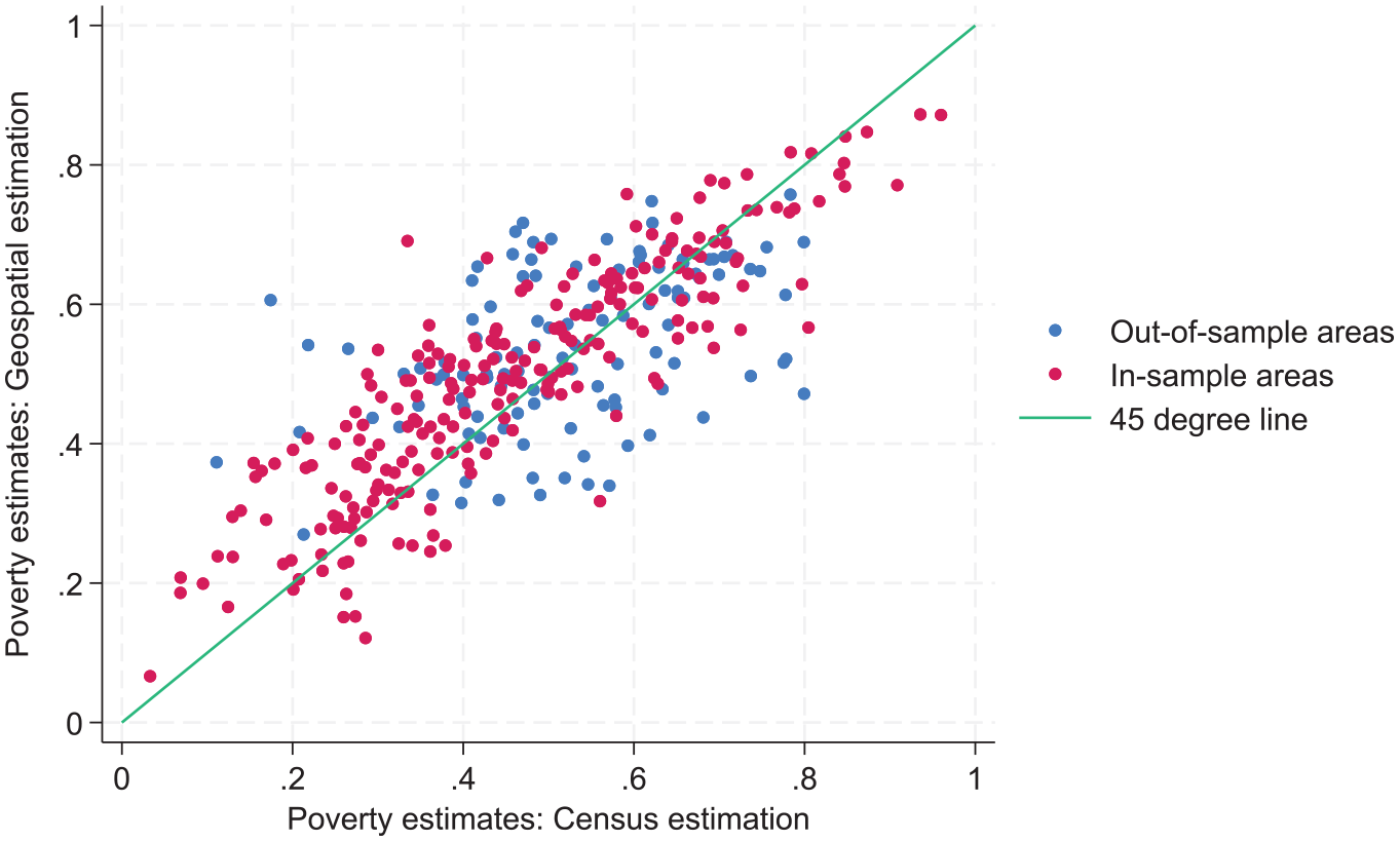
Census-based versus geospatial-based estimates under the unit context model for sampled and non-sampled Communes in Burkina Faso. Red points represent areas (Communes) included in the sample survey, while blue points represent Communes not included in the sample survey.
Looking at the MSE estimates in Table 3, estimates from the household level models have lower MSEs on average compared to the estimates under the grid cell level and area level models. A further comparison between the estimates produced with geospatial covariates and the census-based ones is to compute coverage rates by treating the assumed gold standard census-based estimates as the truth. The coverage rate is the share of Communes for which a 95% normal confidence interval for headcount poverty, defined as the estimate ±1.96 times the square root of the estimated MSE, contains the census-based estimate. Overall, the coverage rate for estimates under the weighted household level model with geospatial covariates is 92.3%. Of course, this is not an ideal test because the census-based estimates are themselves estimates, derived from the same sample data as the geospatial based estimates. Nonetheless, the high coverage rate alleviates concerns about the validity of the estimates produced under the unit context model.
Recent research suggests that machine learning methods that allow for more flexible functional forms can improve small area prediction (Krennmair and Schmid 2022; Merfeld and Newhouse 2023). Exploring whether the use of machine learning methods improves prediction for out-of-sample areas is an area of current research focus. The performance for out-of-sample prediction will depend on the focus country and how well geospatial data predict poverty. Therefore, out-of-sample estimates under the unit context model in the four countries that lack recent census data should be interpreted with great caution and are likely to change when the next round of census-based estimates becomes available.
5. Assessment of Experimental SAE Estimates of Head Count Poverty in Burkina Faso, Chad, Guinea, Mali, and Niger
Having compared geospatial and census-based small area estimates of head count poverty in Burkina Faso, this section describes the generation of experimental small area estimates of head count poverty for all five countries. Estimates are produced using model Equation (1) with geospatial covariates as described in Table A1. Because the estimates we produce are experimental and not official, the results we present do not identify target areas in the focus countries. Model-based estimates under model Equation (1) with geospatial covariates are compared to direct estimates both at target area and at aggregate, regional levels. In addition, MSE estimates of the model-based estimates are compared to the estimated variances of the direct estimates.
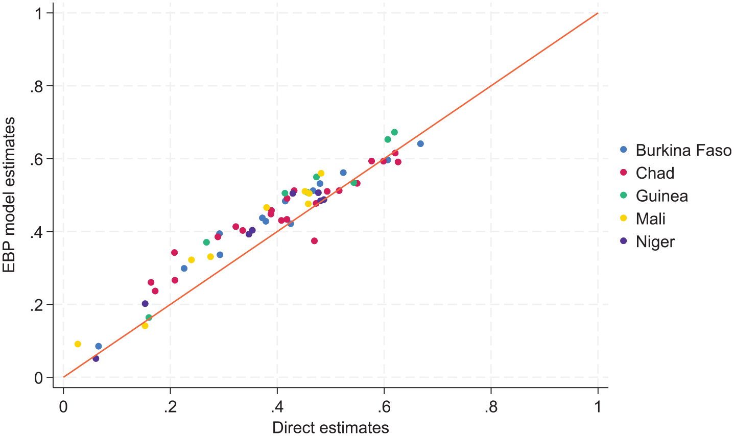
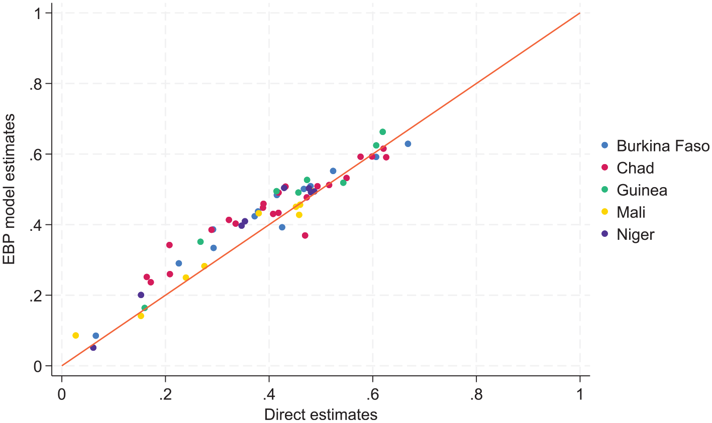
Figure 4 shows the relationship between the EBP estimates under model (1) and the direct estimates at the target area level. In general, model-based estimates are strongly correlated with direct estimates and exhibit less variation than direct estimates, as one would expect due to the impact of shrinkage.
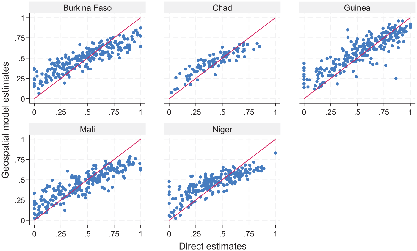
Direct estimates versus model-based (under the unit context model with weighting following Guadarrama et al. (2018)) estimates at target area level.
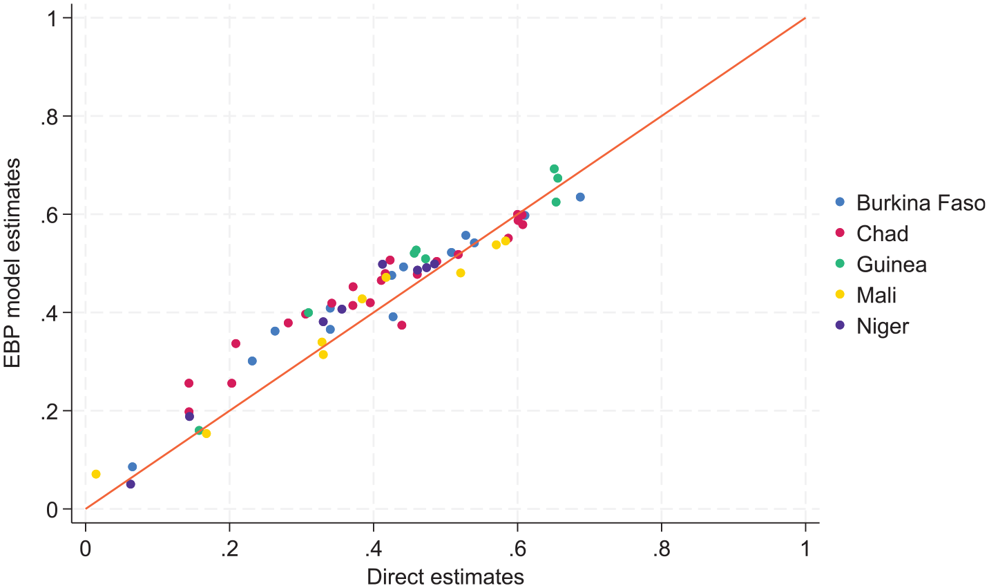
Figure 5 shows the relationship between the EBP estimates under the weighted and unweighted version of model Equation (1). The results show that weighted model-based estimates are systematically higher than the unweighted estimates, while the unweighted estimates are closer to the direct estimates. This may be due to the approach to weighting taken by the Guadarrama et al. (2018) method. In future research it will be interesting to compare the current estimates against estimates obtained by using other weighting methods, including the method that accounts for informative sampling proposed by Cho et al. (2024). For the remaining of this section, we will use the term model-based estimates to refer to those obtained under the unit context model using the weighting proposed in Guadarrama et al. (2018).
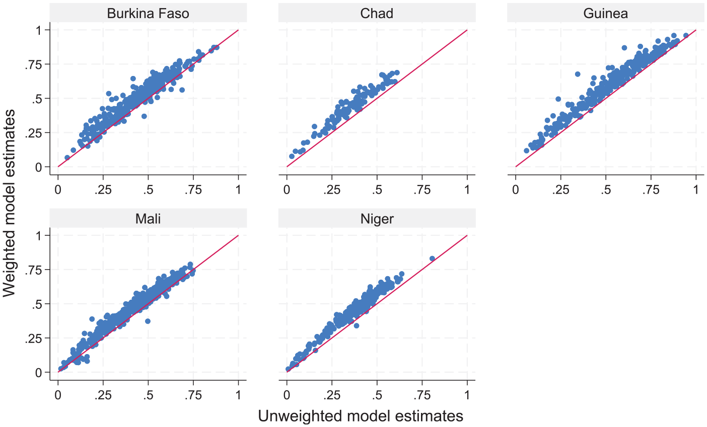
Unweighted model-based estimates versus weighted model-based estimates (under the unit context model with weighting following Guadarrama et al. (2018)) at target area level.
Table 4 presents the median, over target areas, of the coefficient of variation estimated for the model-based versus the direct estimates. Our preferred measure of uncertainty for the direct estimates is based on the Horvitz-Thompson approximation, calculated using the R SAE package, with the sum of the sample weights for each area used to approximate the domain size.
Median cve for Direct and Model-Based Estimates.
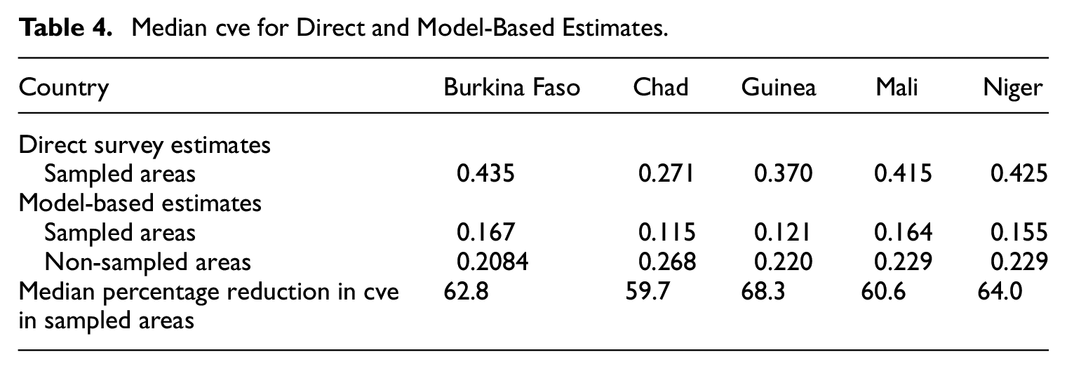
The results in Table 4 show a large reduction in the median cve of the model-based estimates relative to direct estimates. Figure 6 shows reductions in the cve for all but a few target areas. The large efficiency gains from the use of model-based estimates are possibly moderately overestimated. In real data evaluations (e.g., Masaki et al. 2022; Newhouse et al. 2022), coverage rates of confidence intervals produced by using parametric bootstrap MSE estimates are somewhat below the nominal 95%. Nevertheless, even considering this, we expect the model-based estimates to be more efficient than direct estimates.
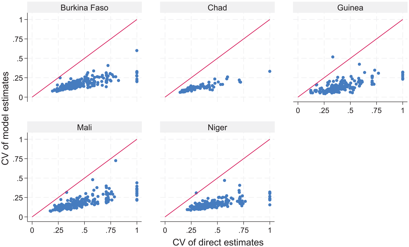
Cve for direct (Horvitz-Thompson approximation) versus cve for model-based estimates for sampled areas by country.
As a further comparison between model-based and direct estimates, we consider a goodness of fit statistic at the target area level, following Brown et al. (2001). The statistic is based on computing Z scores defined as follows,
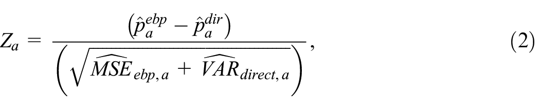
Where
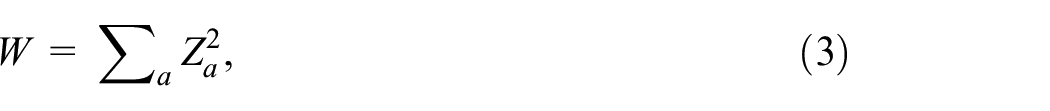
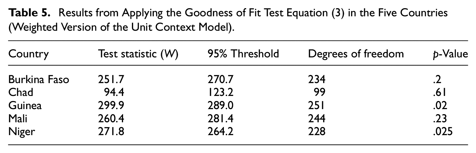
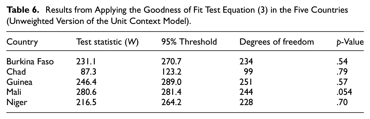
where W has a chi-squared distribution with degrees of freedom equal to the number of areas. A value below the 95% threshold implies a p-value above .05, indicating that the differences are not statistically significant. Table 5 presents the p-value for each country when using the EBP estimates under the weighted version of the unit context model. For Burkina Faso, Chad, and Mali we don’t find statistically significant differences between the model-based and direct estimates. However, this is not the case for Guinea and Niger. Meanwhile, Table 6 presents the p-value for each country when using the EBP estimates under the unweighted version of the unit context model. In this case all p-values exceed .05, indicating that the differences between the direct and EBP estimates are not statistically significant at the 95% level. These results, along with the average poverty estimates reported in Table 3, show the significant impact that weighting can have on model-based estimates and highlight the need for further research on weighting methods.
Results from Applying the Goodness of Fit Test Equation (3) in the Five Countries (Weighted Version of the Unit Context Model).
Results from Applying the Goodness of Fit Test Equation (3) in the Five Countries (Unweighted Version of the Unit Context Model).
Turning now to comparisons at more aggregate levels, Figures 7 to 9 compare the EBP geospatial estimates with direct estimates at the regional level. Figure 8 shows the same results as Figure 7 but excludes out of sample areas when aggregating the EBP estimates at the regional level. We decided to explore this latter approach considering the lower correlation between unit context model estimates and the unit level model estimates for out of sample areas in Burkina Faso. Both Figures 7 and 8 aggregate the model-based estimates using WorldPop weights, while the direct estimates are aggregated using survey weights. Figure 9 remedies this inconsistency by using survey weights when aggregating the model-based estimates from target areas to regions. Overall, the results show that the model-based estimates are aligned well with direct estimates at the regional level. Some discrepancies are to be expected, however, because model-based estimates are affected by shrinkage.
Small area estimates versus direct estimates at regional level (using WorldPop weights for aggregation).
Small area estimates versus direct estimates at regional level (including only in sample target areas and using WorldPop weights for aggregation).
Small area estimates versus direct estimates at regional level (including only in sample target areas and using survey weights for aggregation).
6. Conclusions
This paper describes the methodology used for producing experimental small area estimates of headcount poverty rates in five West African countries where in four of these countries no recent census data are available and zonal statistics from geospatial data sources are available instead. The use of model-based estimation with geospatial covariates offers a pragmatic approach for producing interim model-based estimates because the alternative of using old census data carries risks especially if the distribution of census variables has changed over the intercensal period.
The presence of a recent census in Burkina Faso provided a valuable opportunity to evaluate the results of different models against “gold standard” census-based estimates. In sampled areas, the estimates produced by the unit context model track the census-based estimates well and have lower MSEs than direct estimates. Across all areas, the correlation between the geospatial-based estimates and the census-based estimates is high, but this correlation was much higher in sampled than non-sampled areas. Models specified at the household level generated estimates that were moderately more accurate than those specified at the grid cell level, because the greater variation in per capita consumption allowed for the automated selection of a richer model. Both sets of estimates had lower MSEs than estimates under a model specified at the area level which we think is due to the use of more granular auxiliary data.
Overall, the estimates for the countries without census data show large improvements in MSE reduction compared to direct estimates. In particular, the median cve in sampled areas is reduced between approximately 59% and 68%. The five countries focus of this paper are neighbors and share many economic and social characteristics. Furthermore, all of them implemented highly harmonized surveys concurrently, and the set of geospatial variables available for model selection is identical. However, one cannot be certain that the results for Burkina Faso generalize to the other four West African countries as there are important differences to take into account. Burkina Faso is facing a significant internally displaced people crisis, affecting about 10% of the population, but hosts far fewer refugees than Niger or Chad. Burkina Faso and Guinea lack the large areas of mainly uninhabited desert that characterize Mali, Niger, and Chad. Nonetheless, the relatively low correlation between the geospatial estimates and the census estimates in non-sampled areas observed in Burkina Faso raises the prospect that the estimates for these areas could significantly change when upcoming censuses are collected and combined with survey data to produce updated poverty maps. Given the scarcity of evidence on out-of-sample prediction accuracy in the literature, we recommend treating the out-of-sample estimates in the remaining four countries with a high degree of caution.
There are several additional avenues for further research to inform these types of data integration efforts. These include additional empirical work to validate both point and uncertainty estimates against estimates using recent census data. Zonal statistics derived from geospatial data can be highly correlated. Initial results from current research indicate that the approach used for geospatial data processing and model building with geospatial data can impact on the quality of the produced estimates. Model estimation also matters, it should be possible to improve upon existing methods for estimating mixed models with sampling weights. In addition, exploring the use of machine learning methods to capture complex relationships could improve estimation especially for out-of-sample areas. Despite room for further improvement, the model-based estimates of the type calculated in this paper can provide interim estimates of the spatial distribution of poverty with acceptable uncertainty measures that cannot be obtained with survey data alone.
Footnotes
Appendix A
Appendix B
Appendix C
Appendix D
Acknowledgements
We thank Olivier Dupriez, Jed Friedman, Haishan Fu, Craig Hammer, Johannes Hoogeveen, Gabrela Inchauste, Talip Kilic, Johan Mistiaen, Pierella Paci, and Nobuo Yoshida for their support.
Funding
The author(s) disclosed receipt of the following financial support for the research, authorship, and/or publication of this article: This work was partially supported by the Knowledge for Change Program’s phase IV programmatic research project ‘‘Understanding Trends in Sub-National Differences in Economic Well-Being in Low and Middle- Income Countries’’ Program. The work of Tzavidis, Schmid, and Luna is supported by the Data and Evidence to End Extreme Poverty (DEEP) research programme. DEEP is a consortium of the Universities of Cornell, Copenhagen, and Southampton led by Oxford Policy Management, in partnership with the World Bank - Development Data Group and funded by the UK Foreign, Commonwealth and Development Office. The work of Tzavidis is also supported by the UKRI-ESRC strategic research grant ES/X014150/1 for ‘‘Survey data collection methods collaboration: securing the future of social surveys’’, known as Survey Futures. Survey Futures is a collaboration of twelve organisations, benefitting from additional support from the Office for National Statistics and the ESRC National Centre for Research Methods. Further information can be found at www.surveyfutures.net.
Received: September 2023
Accepted: August 2024