Audit samples are selected by businesses, institutions, government agencies, and other organizations to check the accuracy of financial reports and assess the quality of services provided among other reasons. A standard design used in auditing is stratified simple random sampling. Point estimates and confidence intervals for population values are usual products of an audit. Cochran’s sample size rule and its extension by Sugden, Smith, and Jones provided minimum sample size formulas for a simple random sample to ensure effective normal approximation and adequate coverage for nominal 95% confidence intervals of a standardized or Studentized sample mean. The purpose of this paper is to extend Cochran’s rule and establish a formula for the minimum sample size for the normal approximation and the use of traditional one-sided or two-sided confidence intervals to be acceptable for mean estimation in stratified simple random samples. We concentrate on variables that are at least partially continuous. Simulations are used to examine the performance of our sample size formula with a variety of skewed populations based on ones encountered in auditing.
In audits of financial accounts, patient medical records, program effectiveness, and internal business operations, statistical sampling may be used when a population is too large to economically conduct a census. The International Standard on Auditing (Financial Reporting Council 2022) gives general guidance on audit sampling, including sample size specification. The United Kingdom’s National Health Service allows sampling when assessing how well patient care is given (UH Bristol and Weston Clinical Audit Team 2022). In Canada, sampling can be used in consumer tax audits (Ministry of Finance 2014). In its Revenue Procedure 2011-42 and in other advisory notes issued by the United States Internal Revenue Service (U.S. Internal Revenue Service 2011), the IRS allows statistical sampling to be used to estimate some quantities needed for tax filing. Examples are estimation of stock basis for shares of stock acquired in transfer transactions, establishing the amount of deductible meal and entertainment (M&E) expenses, evaluation of qualified research expenditures in company research and development (R&D) activities, and acceleration of capital assets into different lifespans to depreciate their values over different numbers of years under the tangible property regulations (TPR).
To be acceptable to the US IRS, a taxpayer must adhere to a series of technical requirements. Probability sampling must be used, and the sampling frame must cover the entire relevant population of financial items. IRS then generally requires that a taxpayer use what it terms “the least advantageous 95% one-sided confidence limit” for whatever is being estimated. By “least advantageous” IRS means either the upper or lower limit of the normal approximation confidence interval that results in the least benefit to the taxpayer. An exception to this is if the estimator, , is sufficiently precise. The IRS criterion is that the point estimate can be used if the relative precision of is 0.10 or smaller. IRS defines the relative precision as either (a) , where is the 95th percentile of the Student’s t-distribution with appropriate degrees of freedom (df) and is the estimated variance of , when the total sample size is less than 100, or (b) as when the total sample size is greater than or equal to 100 where 1.645 is the 95th percentile of the standard normal distribution. If the relative precision is between 0.10 and 0.15, a sliding scale between the point estimate and the 95% one-sided confidence limit can be used on a tax return.
The US IRS also restricts the types of sample designs and estimators of means or totals that can be used. Simple random sampling and stratified simple random sampling are permitted along with the expansion estimator, difference estimator, and ratio and regression estimators. The relative precision criterion is premised on a normal approximation confidence interval being appropriate. Because of the penalty imposed for an imprecise estimator, a taxpayer also has an incentive to use a sample size large enough so that the precision standard, , is achieved.
Another implicit requirement is that the sample be large enough that a normal approximation confidence interval (CI) has the desired coverage probability. For example, a one-sided 95% CI should include the population value in 95% of samples if the sampling and estimation procedure were repeated many times. Thus, in addition to meeting the precision criterion above, a sample should be sufficiently large that the normal approximation CIs have the desired coverage rates. Determining that sample size is the subject of this paper.
A common sample design, especially for audit and business surveys, is stratified simple random sampling (STSRS). Methods of allocating a sample to the strata are covered in standard textbooks (e.g., see Cochran 1977; Lohr 2009; Valliant et al. 2018). The methods used in business surveys are reviewed more generally in the collections edited by Cox et al. (1995) and Snijkers et al. (2013).
Section 2 reviews basic results on large sample normality for simple random samples and previous work on determining how large the size of a simple random sample must be to achieve approximate normality of estimators. Section 3 presents Edgeworth approximation theory that leads to a new rule for determining the sample size in STSRS. Section 4 discusses simulation studies that verify the usefulness of the rule. Section 5 is a conclusion.
2. Notation and Basic Results
Let be the quantities that belong to a finite population and be the sample of from . For simple random sampling without replacement (SRSWOR) from a finite population, the sample mean, , is an unbiased estimator of population mean, . The variance of in SRSWOR is , where and . This variance is estimated by , where . Obtaining the exact distribution of or of is difficult, as the distribution of y in the population is often unknown. However, under certain regularity conditions, the finite population central limit theorem (CLT) holds: if the sample size is sufficiently large, the distribution of will be approximately normal. Madow (1948), Erdos and Renyi (1959), Hajek (1960), and Rosen (1972) provided various forms of finite population CLTs for SRSWOR. Also see Lehmann (1999) Theorem 2.8.2 for a detailed derivation of a convenient form. For designs more complex than SRSWOR, authors often assume that first-stage units are selected with replacement to obtain design-based, that is, repeated sampling, results (e.g., see Krewski and Rao 1981; Rao and Wu 1988).
Although asymptotic normality can be established under certain conditions, a practical question that sampling practitioners often ask is: how large of a sample size is sufficient for the normal approximation to be acceptable? Some textbooks of introductory statistics use the “magic” number of as the minimum sample size to ensure the Studentized statistic, , has an approximately normal distribution, which often does not suffice for highly skewed populations.
Cochran (1977, 42) described a crude rule for how large the sample size needs to be for normal approximation as
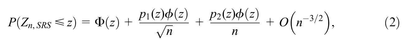
where is Fisher’s measure of skewness. To derive this rule, Sugden et al. (2000) used a three-term Edgeworth expansion of the standardized statistic , assuming both and excess kurtosis are equal to 0. The expansion approximates the cumulative distribution function (CDF) of as
where and are the CDF and probability density function (PDF) of a standard normal random variable respectively, , and . Then by ignoring the error term in Equation (2) and solving the two inequalities and , Cochran’s sample size rule Equation (1) was obtained. Note that the two inequalities are sufficient but not necessary to ensure the coverage probability of the nominal 95% confidence interval is at least 94%, based on the normal distribution approximation with known population variance.
Sugden et al. (2000) also extended Cochran’s rule and provided the minimum SRSWOR sample size for normal approximation of the Studentized statistic, , as
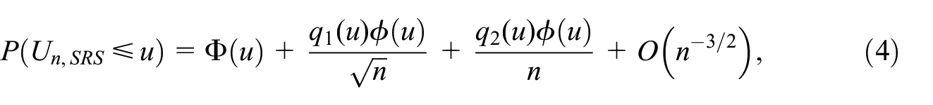
which added 28 extra sampling units to Cochran’s rule, as a penalty for not knowing the true variance of the sample mean. Equation (3) was derived using a three-term Edgeworth expansion of the studentized statistic , obtained in Sugden and Smith (1997) and again assuming both and are equal to 0. The approximation is
where and . Note that Sugden and Smith (1997) used techniques in Hall (1992, Section 2.4) to establish Equation (4) formally, but stated that a further argument invoking say, the non-lattice condition from Robinson (1978) or Cramer’s condition (Cramer 1962, Chapter IV) is needed to establish Equation (4) rigorously as an asymptotic expansion.
Equation (3) was then obtained by again ignoring the error term but alternatively solving a single inequality , which ensures 94% coverage probability for a two-sided 95% nominal confidence interval, based on the normal distribution approximation with sample variance, but does not guarantee coverages for one-sided confidence intervals from either side. Equation (3) then provides a justification for the minimum sample size of 30 in an SRS in many introductory textbooks, assuming the population skewness is small.
The finite population CLT can be extended to the sample mean of a stratified simple random sample (STSRS) with L strata, defined as , where and are the population and sample size in stratum respectively and is the sample mean in stratum , with the being the sample in stratum h. The mean is also an unbiased estimator of the population mean, , where is the population in stratum .
As Lohr (2009, p. 79) mentions, the distribution of will be approximately normal with the support of the finite population CLT, if either (a) within each stratum the sample size is large, or (b) the number of strata is large. Krewski and Rao (1981) give conditions on population moments and other quantities under which a CLT for stratified sampling holds. Some practitioners, especially in tax and audit sampling industries, adhere to a minimum sample size of 30 units per stratum to ensure the normal approximation is deemed acceptable, which again may be insufficient for some cases while excessive for others.
3. Edgeworth Theory for Stratified Sampling
In this section, we use an Edgeworth expansion for a stratified sample to derive a new sample size formula similar to Cochran’s for STSRS with bounded L, with a simplified form by considering Neyman allocation (Neyman 1934), which is common in tax and business sampling as the practitioners have an incentive to minimize the variance of an estimator. The results also hold for other allocations to strata like proportional, equal, and cost-contrained as discussed in the Appendix. The stratified mean, , is a sum of independent, non-identically distributed random variables, unlike the mean in simple random sampling which is a sum of independent, identically distributed (iid) variables. The Edgeworth theory available for the non-iid case is more limited than for the iid case.
3.1. Notations and Assumptions
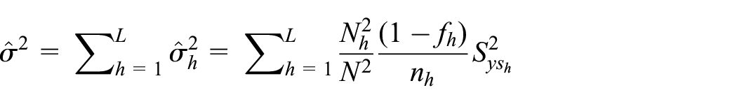
First, we present additional notation. For STSRS with bounded L, let
be the unbiased estimator of the design variance of :
where , , , and is the population mean in stratum h.
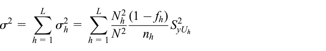
For the asymptotic properties, we assume there is a sequence of finite stratified populations all with strata and population size in each stratum , and sample size as (e.g., see Fuller 2009). For simplicity, the index is suppressed moving forward.
We obtain the Edgeworth expansion needed for the new sample size formula under the conditions below for all (see Chen and Sitter 1993):
and remains bounded as .
is bounded for .
There exist and , which satisfy for some , such that for any fixed , the number of indices for which for all and all integer is greater than for all , where .
and the allocation are all bounded away from 0.
Condition (a) ensures that the standardized statistic of , given by and the Studentized statistic of , given by both converge to a normal distribution when for each stratum , based on Lehmann (1999, Theorem 2.8.2) and Li and Ding (2017, Proposition 1). Conditions (a) and (b) also ensure that and , which is the th population moment of the mean of stratum , are both bounded. Conditions (b) and (c) were presented in Chen and Sitter (1993) as the conditions for the two-term asymptotic Edgeworth expansion for when L is bounded. Although the non-lattice condition (c) seems quite complex, it does have an intuitive interpretation first given by Robinson (1978) for SRSWOR, which is to “ensure the values of ( in our notation) in stratum do not cluster around too few values.” Condition (c) is fine for many quantities collected in audit populations which are continuous expense amounts, but the condition is not suitable for proportion estimation. For example, if y is 1 or 0 depending on whether a reported financial item was erroneous or not, then condition 3 will not hold.
3.2. Edgeworth Expansion for a Standardized Statistic with Known Stratum Variances
With the conditions mentioned above, we will use a two-term Edgeworth expansion for the cumulative distribution of provided by Chen and Sitter (1993). The expansion is written as
where and are the cumulative distribution function (CDF) and probability density function (PDF) of a standard normal distribution respectively, and .
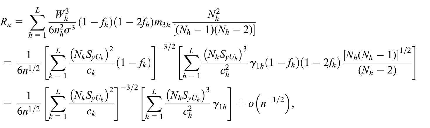
Furthermore, let be the population skewness of stratum , which is also bounded by condition (b). With and bounded away from 0, we have . Thus,
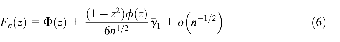
and we can simplify the Edgeworth expansion in Equation (5) into
where and .
Note that Equation (6) is a two-term expansion for contrary to the three-term expansions for in Equation (2), and when , the second term of in Equation (6) is the same as the second term in Equation (2). A three-term Edgeworth expansion for is not available in the literature, implying that the steps used in finding an SRS sample size cannot be entirely replicated. Following the derivation of Cochran’s rule Equation (1) by Sugden et al. (2000), we also use a two-inequality approach: for a small , we require an expansion for the cumulative distribution of , such that
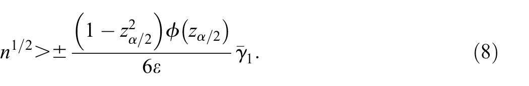
where is the th percentile of the standard normal distribution. This will ensure that a one-sided confidence interval has the coverage probability of at least , and a two-sided confidence interval has the coverage probability of at least . If n is large enough that we can ignore the error term of the expansion in Equation (6), then the distribution function, , will be approximately normal plus the skewness adjustment in the second term. When the term is negligible, the two inequalities in Equation (7) lead to
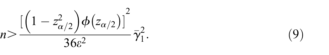
Obviously, depending on the sign of , one of the inequalities will always hold, which indicates, either with lower bound or upper bound, one of the one-sided confidence intervals will always have coverage probability of at least , regardless of how large is. Still, we can unify these two inequalities in Equation (8) by taking a square on both sides:
If we set to 0.05 and to 0.005, which would also make the coverage probability for the two-sided 95% confidence interval at least 94%, Equation (9) becomes . When , this is slightly more conservative than Cochran’s rule Equation (1), as a trade-off of using a two-term instead of a three-term expansion and being easier to calculate the sample size formula with general and .
3.3. Edgeworth Expansion for a Studentized Statistic with Estimated Stratum Variances
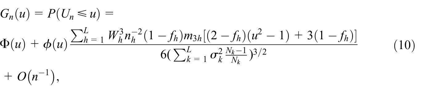
Next, we pivot to the Studentized statistic In practice, is used far more frequently than , as the population variance is usually unknown. Mirakhmedov et al. (2015, Section 3) provided a two-term Edgeworth expansion for , given by
which was established formally using a procedure similar to that outlined in Sugden and Smith (1997).
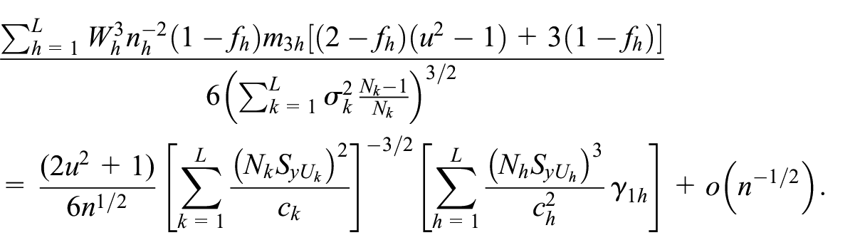
Again assuming that and is bounded away from 0, similar to the deduction process for in (5), the second term on the right-hand side of Equation (10) becomes
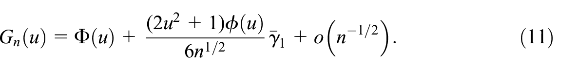
Thus, Equation (10) can be simplified into
where is the same as defined below (6).
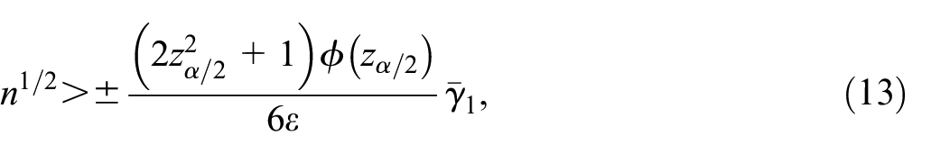
While we cannot use the one-inequality approach of to get the minimum sample size formula for a two-term expansion, we can still use the two-inequality approach used to obtain Equation (1) and Equation (9): for a small , we require an expansion for the cumulative distribution of , such that
When the term is negligible, the two inequalities in Equation (7) become
and we can unify these two inequalities into:
where When , , and , Equation (14) becomes , which is much more conservative than Equation (3). This is also contrary to the relationship between expressions Equation (9) and Equation (1) for the same special case. However, Equation (14) has the benefit of being able to control the coverage probability for both one-sided confidence intervals with lower or upper bound, which is critical in tax sampling regulations. Admittedly, the improvement in coverage for one-sided confidence intervals does not always justify the cost of sample size increase. Nonetheless, in the context of audit sampling, one-sided confidence interval coverage is a necessity due to the auditors’ objective to preclude taxpayers from claiming undue benefits, rather than the converse.
3.4. Neyman Allocation Application
If the sample size in each stratum is determined by Neyman allocation (Neyman 1934), that is , then in Equation (9) and Equation (14), we have and therefore is the weighted average population skewness across all strata. We will focus on the Neyman allocation and examine the performance of rule Equation (14) through simulation illustrated in the next section. However, Equation (9) and Equation (14) are general formulas that apply to a variety of allocations to strata as illustrated in the Appendix.
The rule in Equation (14) gives us a few thoughts: (1) it provides a minimum total sample size for STSRS with a wide variety of allocations. Thus, no matter how many strata there are, as long as the total sample size exceeds the threshold, the coverage probability based on the normal approximation is sufficient; (2) it supports the statement in Lohr (2009, p. 79) that the normal approximation for STSRS works if either the sample size for each stratum is large or the number of strata is large; and (3) stratification, when done efficiently to shrink skewness, can reduce the sample size needed significantly for the normal approximation to work.
4. Simulation
The motivation for our simulation setup is tax and audit sampling. As noted in Section 1, the U.S. Internal Revenue Service (IRS 2011) allows STSRS to be used to estimate some quantities needed for tax filing. We generated several populations that are based on ones encountered in tax auditing work in which the y variable is continuous, but a portion of the items in the population are zeroes, as described in detail below. Samples were repeatedly selected from each of the populations and empirical coverage rates of confidence intervals calculated.
Six populations were used in the simulations and were derived from tax populations that the first author has encountered. Some data points were masked to protect confidentiality. The sampling units in the populations were records (expenses, employees, assets, etc.) with a monetary y-value (invoice values, wages, capital cost, etc.), which are like quantitative variables found in business and institutional populations and are all highly skewed before stratification.
The performance of the minimum sample size rule in Equation (14) was evaluated empirically through simulations. To apply rule Equation (14), the parameter was set to be 0.05 and the error term was set to be either 0.005 or 0.01. The parameter settings should theoretically ensure the undercoverage for two-sided 95% confidence intervals to be less than 1% or 2%, respectively. Also note that in Equation (14), and , which indicates that the parameter settings should also ensure the undercoverage for one-sided 95% confidence interval with lower or upper bound to be less than 0.65% and 1.30% respectively.
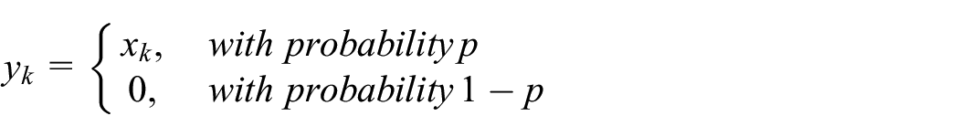
For the sake of simplicity and to closely align with real-world practices, each population was stratified by the range of the positive monetary amount, denoted as , into four to six strata, ensuring that the total monetary amount of each stratum was approximately equal and the population size in each stratum was not too small. The y-variables were generated through an all-or-nothing distribution of
which is very common in tax records and is referred to as a hurdle model in economics (Cragg 1971). A hurdle model satisfies the non-lattice condition (c) in Subsection 3.1; is also termed “partially continuous” here. The prototypical example in a tax population is that some expense items may qualify for a tax credit or deduction when filing an income tax form while others do not. Similar situations occur in populations of consumer purchases of durable goods, for example, automobiles, in a calendar quarter where some consumers make a purchase, but many do not. Similarly, in a calendar quarter, a family may have a medical expense for hospitalization, but others do not.
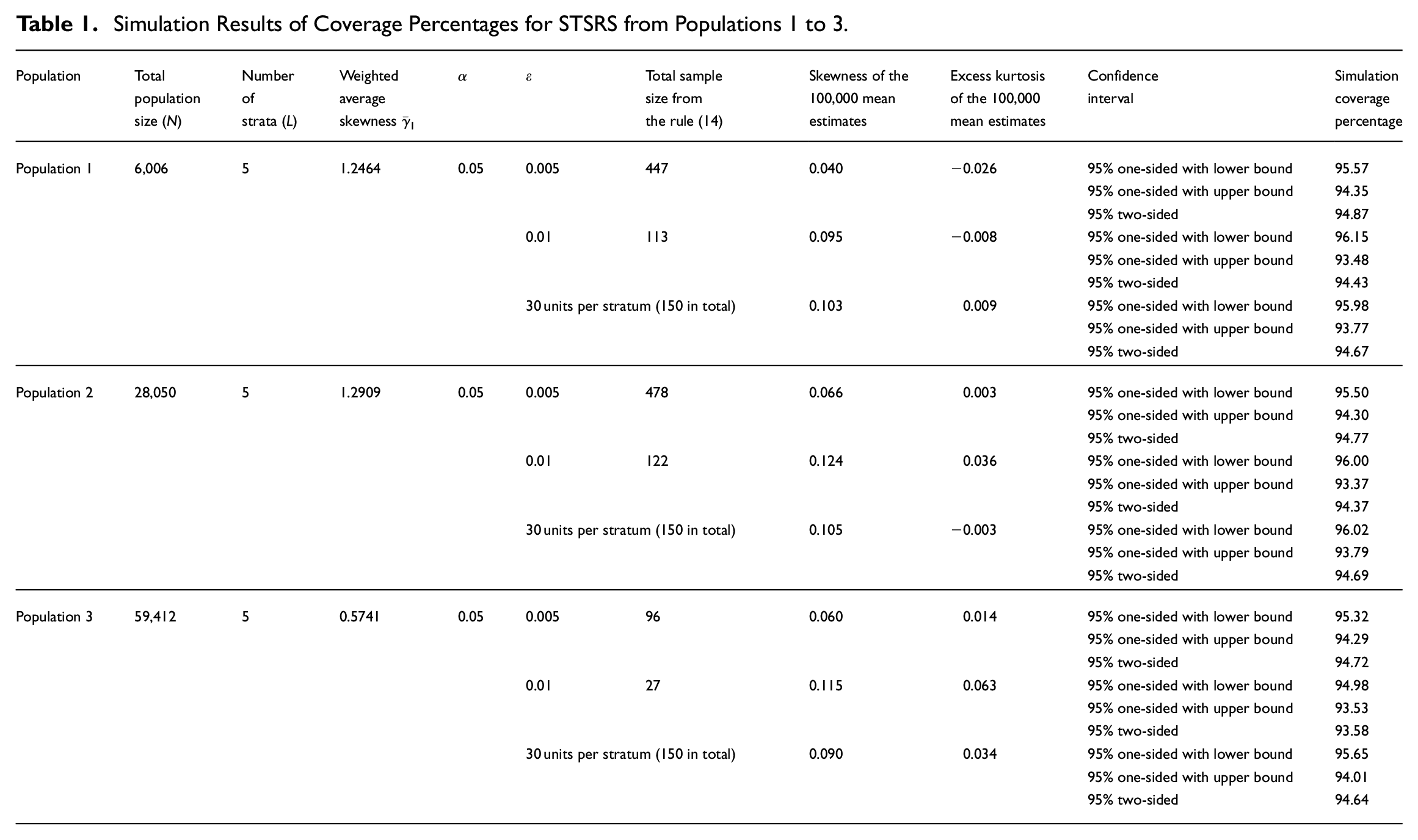
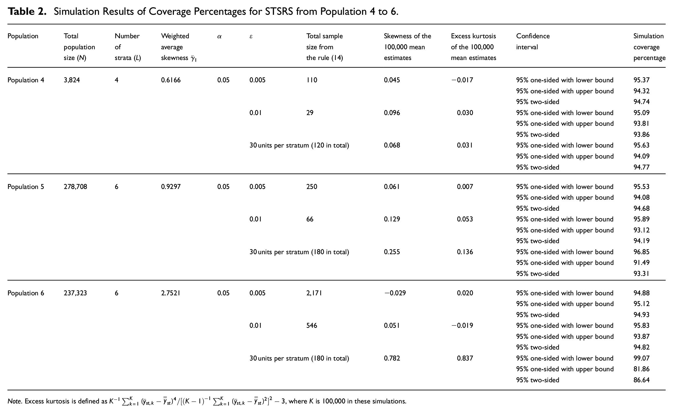
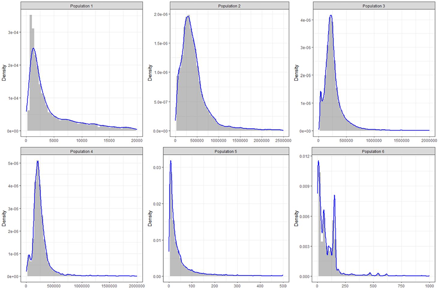
The qualifying probability was set to be 30% for populations 1 and 2, 60% for populations 3 and 4, and 90% for populations 5 and 6. The sizes of the populations are given in Tables 1 and 2. Figure 1 shows the histograms for the six populations used in the simulations. To enhance the clarity and readability of the graphs, extremely large values were excluded from the data prior to plotting; the large values in each population were retained for the simulations. Although Sugden et al. (2000, p. 788) point out that a few outliers can have a damaging effect on coverage probabilities of confidence intervals, the large y values were not so extreme as to affect results here. For each of the six populations, the standard deviation and population skewness in each stratum were calculated, and the sample size for each stratum was determined using the rule Equation (14) as well as the Neyman allocation. In addition, for comparison purposes, an alternative sample size method of 30 units per stratum was used for each sample design. For each population and sample size scenario, 100,000 simulations of STSRS selections were conducted, and the coverage percentages were summarized.
Simulation Results of Coverage Percentages for STSRS from Populations 1 to 3.
Population
Total population size (N)
Number of strata (L)
Weighted average skewness
Total sample size from the rule (14)
Skewness of the 100,000 mean estimates
Excess kurtosis of the 100,000 mean estimates
Confidence interval
Simulation coverage percentage
Population 1
6,006
5
1.2464
0.05
0.005
447
0.040
−0.026
95% one-sided with lower bound
95.57
95% one-sided with upper bound
94.35
95% two-sided
94.87
0.01
113
0.095
−0.008
95% one-sided with lower bound
96.15
95% one-sided with upper bound
93.48
95% two-sided
94.43
30 units per stratum (150 in total)
0.103
0.009
95% one-sided with lower bound
95.98
95% one-sided with upper bound
93.77
95% two-sided
94.67
Population 2
28,050
5
1.2909
0.05
0.005
478
0.066
0.003
95% one-sided with lower bound
95.50
95% one-sided with upper bound
94.30
95% two-sided
94.77
0.01
122
0.124
0.036
95% one-sided with lower bound
96.00
95% one-sided with upper bound
93.37
95% two-sided
94.37
30 units per stratum (150 in total)
0.105
−0.003
95% one-sided with lower bound
96.02
95% one-sided with upper bound
93.79
95% two-sided
94.69
Population 3
59,412
5
0.5741
0.05
0.005
96
0.060
0.014
95% one-sided with lower bound
95.32
95% one-sided with upper bound
94.29
95% two-sided
94.72
0.01
27
0.115
0.063
95% one-sided with lower bound
94.98
95% one-sided with upper bound
93.53
95% two-sided
93.58
30 units per stratum (150 in total)
0.090
0.034
95% one-sided with lower bound
95.65
95% one-sided with upper bound
94.01
95% two-sided
94.64
Simulation Results of Coverage Percentages for STSRS from Population 4 to 6.
Population
Total population size (N)
Number of strata (L)
Weighted average skewness
Total sample size from the rule (14)
Skewness of the 100,000 mean estimates
Excess kurtosis of the 100,000 mean estimates
Confidence interval
Simulation coverage percentage
Population 4
3,824
4
0.6166
0.05
0.005
110
0.045
−0.017
95% one-sided with lower bound
95.37
95% one-sided with upper bound
94.32
95% two-sided
94.74
0.01
29
0.096
0.030
95% one-sided with lower bound
95.09
95% one-sided with upper bound
93.81
95% two-sided
93.86
30 units per stratum (120 in total)
0.068
0.031
95% one-sided with lower bound
95.63
95% one-sided with upper bound
94.09
95% two-sided
94.77
Population 5
278,708
6
0.9297
0.05
0.005
250
0.061
0.007
95% one-sided with lower bound
95.53
95% one-sided with upper bound
94.08
95% two-sided
94.68
0.01
66
0.129
0.053
95% one-sided with lower bound
95.89
95% one-sided with upper bound
93.12
95% two-sided
94.19
30 units per stratum (180 in total)
0.255
0.136
95% one-sided with lower bound
96.85
95% one-sided with upper bound
91.49
95% two-sided
93.31
Population 6
237,323
6
2.7521
0.05
0.005
2,171
−0.029
0.020
95% one-sided with lower bound
94.88
95% one-sided with upper bound
95.12
95% two-sided
94.93
0.01
546
0.051
−0.019
95% one-sided with lower bound
95.83
95% one-sided with upper bound
93.87
95% two-sided
94.82
30 units per stratum (180 in total)
0.782
0.837
95% one-sided with lower bound
99.07
95% one-sided with upper bound
81.86
95% two-sided
86.64
Note. Excess kurtosis is defined as , where is 100,000 in these simulations.
Histograms with density estimates for the six populations used in simulations.
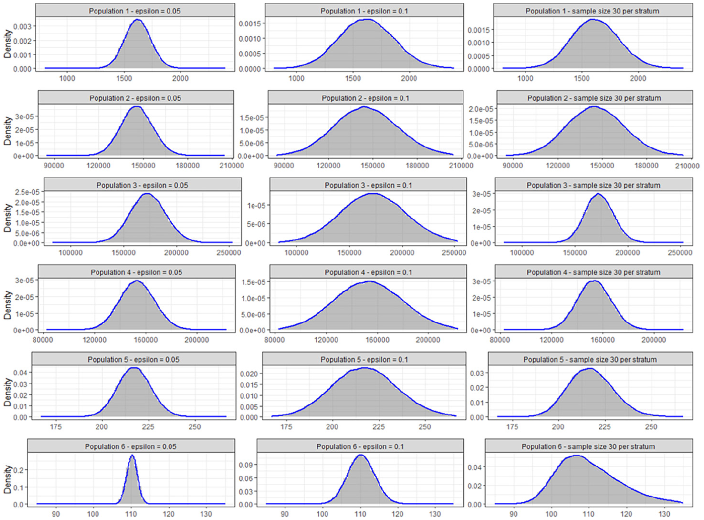
As Tables 1 and 2 show below, for all populations and sample designs in the simulation, the minimum sample size given by rule Equation (14) provided adequate coverage compared to the theoretical value, which is either 94% or 93% for the two-sided 95% confidence intervals, and 94.35% or 93.70% for the one-sided 95% confidence intervals with lower or upper bounds. Also, the skewness and the excess kurtosis of the mean estimates from the 100,000 simulations for each sample size scenario were close to zero when rule Equation (14) is used, demonstrating strong normality. For populations 1 to 4, with significantly smaller sample sizes, the samples with sample size determined by rule Equation (14) when provided similar coverage probability to the samples with 30 units per stratum. For populations 5 and 6, the method of 30 units per stratum failed to provide adequate coverage while our new rule did result in confidence intervals with nearly nominal coverage. In both populations 5 and 6, the skewnesses and excess kurtoses are considerably different from zero for the 30 units per stratum designs. Therefore, rule Equation (14) substantially outperformed the method of 30 units per stratum in achieving normality of the estimator of the mean.
Note that for all the populations, we assume the variable of interest is available for the entire population so that the parameters of standard deviation and the population skewness in each stratum can be calculated. While that is rarely the case in practice, if can be linked to an auxiliary variable , which is available for the population, through a probabilistic model like the all-or-nothing distribution shown above, the parameters of and can be estimated through either analytical derivation or simulations.
Figure 2 below shows the histograms of mean estimates for each of the six populations for the different sample size scenarios. Density estimates were superimposed on each histogram. The first two columns show the distributions of the mean estimates generated by the 100,000 samples with the sample sizes determined by rule Equation (14), while the third column shows the distribution of the mean estimates generated by the samples with 30 sample units per stratum. For population 5 and 6, the distributions of the 100,000 estimates from the method of 30 units per stratum were skewed and depart from normality.
Histograms of the mean estimates from 100,000 simulations for different sample size scenarios.
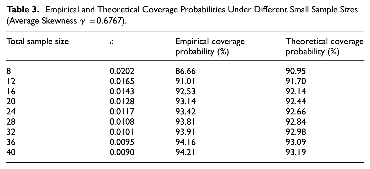
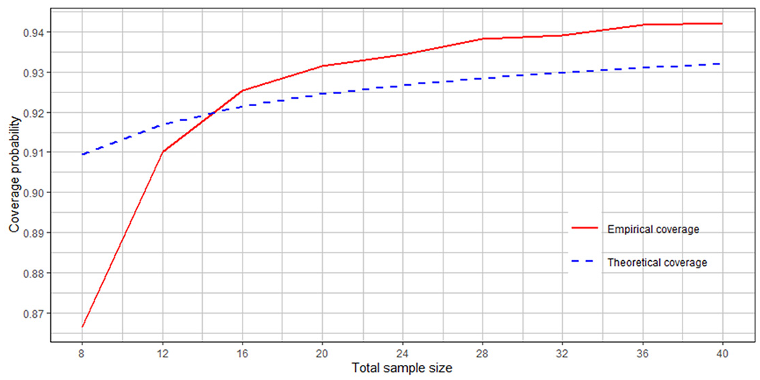
Finally, rule Equation (14) requires that the term be negligible in Equation (11). Population 3 was used as an example to examine the impact of small sample size on this rule. For the simplicity of the stratum sample size determinations, the population was re-designed to have four strata with approximately equal in each stratum, which ensures equal sample size per stratum with Neyman allocation. 100,000 simulations of stratified simple random sample selections were then conducted with total sample sizes ranging from 8 to 40 in increments of 4, which is equivalent to the sample size per stratum ranging from 2 to 10 in increments of 1. The undercoverage error term is calculated by reversing Equation (14): , which provides a benchmark for theoretical undercoverage when compared to the empirical undercoverage. The coverage percentages of two-sided, normal approximation 95% confidence intervals of the sample mean were summarized and are shown in Table 3. Although the sample sizes are small, we use normal approximation confidence intervals since rule Equation (14) is based on the normal distribution. Use of confidence intervals with t-statistics would produce wider intervals and even higher empirical coverage rates.
Empirical and Theoretical Coverage Probabilities Under Different Small Sample Sizes (Average Skewness ).
Total sample size
Empirical coverage probability (%)
Theoretical coverage probability (%)
8
0.0202
86.66
90.95
12
0.0165
91.01
91.70
16
0.0143
92.53
92.14
20
0.0128
93.14
92.44
24
0.0117
93.42
92.66
28
0.0108
93.81
92.84
32
0.0101
93.91
92.98
36
0.0095
94.16
93.09
40
0.0090
94.21
93.19
Figure 3 is a plot of the empirical coverage rates (labeled “Empirical coverage”) and “Theoretical coverage” values calculated as , based on the inequalities in Equation (12), versus the total sample sizes. Figure 3 shows that, for this 4-strata sample design, rule Equation (14) works very well even for small sample sizes. For all sizes greater than or equal to 16, the empirical coverage probability is no worse than the theoretical one.
Empirical versus theoretical coverage probability in population 3 under rule (14).
Conclusion
This paper has developed a rule in Equation (14) that is similar to both Cochran’s original in Equation (1) and the extended rule in Equation (3) provided by Sugden et al. (2000) for the standardized or Studentized sample mean of STSRS for variables that are partially continuous, or that at least do not cluster around too few values. The new rule applies to a stratified sample size determined by a variety of allocations. This rule was derived using a two-term Edgeworth expansion and provided the minimum sample size for sufficient coverage of traditional one-sided or two-sided confidence intervals using the normal approximation.
We examined the performance of the rule through simulations and demonstrated that for a STSRS with Neyman allocation, when the sample size satisfies this rule, the mean estimate has strong normality and the one- and two-sided, normal approximation confidence intervals cover population values at the desired rates, which is an error term away from the nominal coverage probabilities. The error is a tolerance for how close the achieved confidence interval coverage should be to the nominal value. The tolerance can be controlled when calculating the sample size. The performance of the rule was also compared to an alternative, rule-of-thumb method of 30 units per stratum and was shown to significantly outperform the latter approach.
An important caveat is that our sample size formulas do not apply directly to estimates of binary characteristics (as studied, e.g., by Kott and Liu 2009) since the assumptions for the Edgeworth approximation we have used require that the y’s do not cluster on too few values. The rule Equation (14) could potentially be improved by using a three-term Edgeworth expansion for . A three term Edgeworth expansion takes kurtosis and the secondary effect of skewness into consideration and thus potentially provides a more accurate minimum sample size threshold. That development will be left for further research.
Footnotes
Appendix
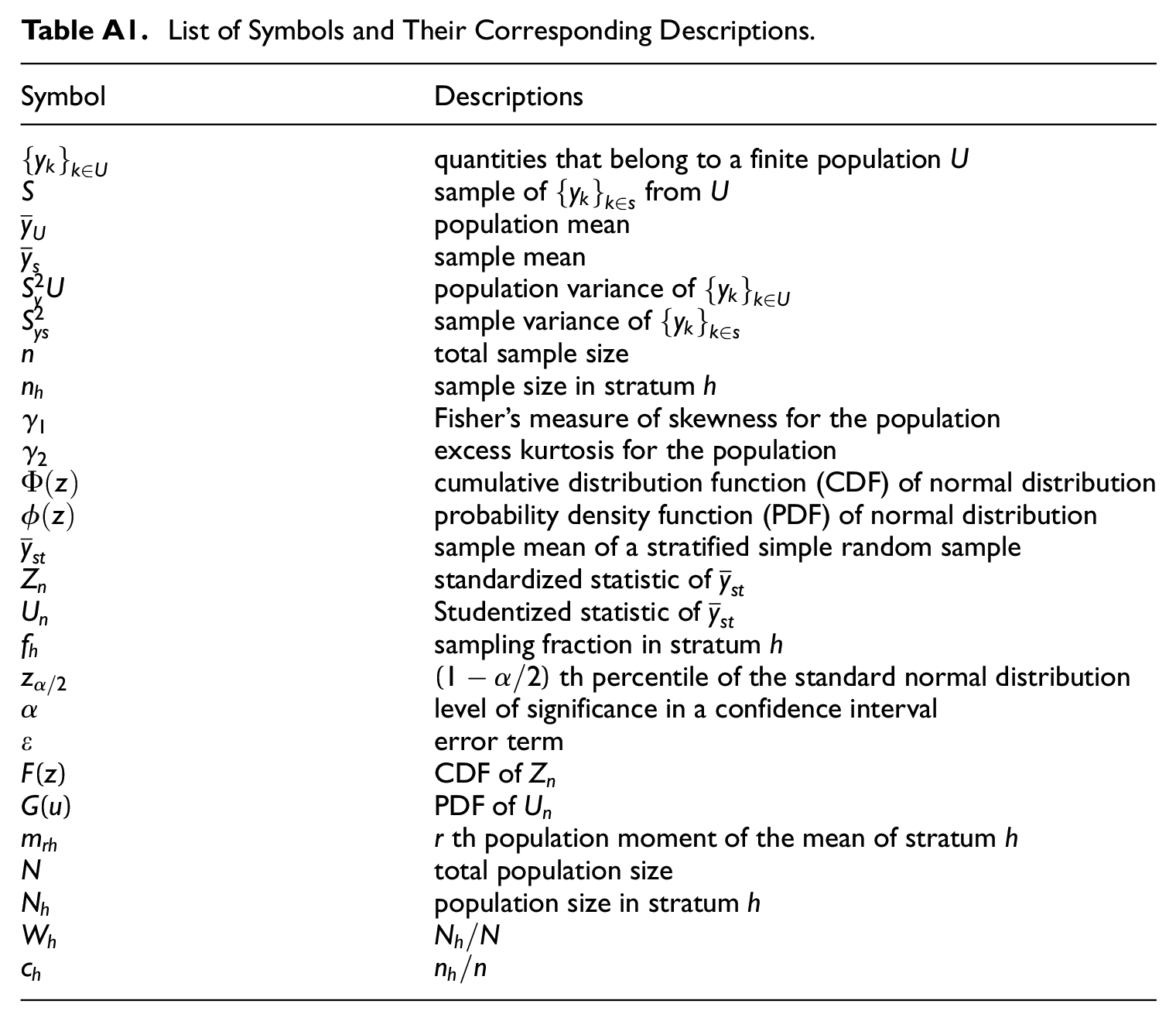
List of Symbols and Their Corresponding Descriptions.
Symbol
Descriptions
quantities that belong to a finite population
sample of from
population mean
sample mean
population variance of
sample variance of
total sample size
sample size in stratum h
Fisher’s measure of skewness for the population
excess kurtosis for the population
cumulative distribution function (CDF) of normal distribution
probability density function (PDF) of normal distribution
sample mean of a stratified simple random sample
standardized statistic of
Studentized statistic of
sampling fraction in stratum h
th percentile of the standard normal distribution
level of significance in a confidence interval
error term
CDF of
PDF of
th population moment of the mean of stratum h
total population size
population size in stratum h
Acknowledgements
The authors are grateful to their colleagues Ryan Petska and Ed Cohen for their valuable input and comments that helped getting the paper to the present form.
Funding
The author(s) received no financial support for the research, authorship, and/or publication of this article.
ORCID iD
Siyu Qing
Received: November 2023
Accepted: March 2024
References
1.
ChenJ.SitterR.1993. “Edgeworth Expansion and the Bootstrap for Stratified Sampling Without Replacement from a Finite Population.”The Canadian Journal of Statistics21 (4): 347–57. DOI: https://doi.org/10.2307/3315699.
2.
CochranW. G.1977. Sampling Techniques. 3rd ed. New York, NY: Wiley.
3.
CoxB. G.BinderD. A.ChinnappaB. N.ChristiansonA.ColledgeM. J.KottP. S.1995. Business Survey Methods. New York, NY: John Wiley & Sons.
4.
CraggJ. G.1971. “Some Statistical Models for Limited Dependent Variables with Application to the Demand for Durable Goods.”Econometrica39 (5): 829–44. DOI: https://doi.org/10.2307/1909582.
5.
CramerH.1962. Random Variables and Probability Distributions. 2nd ed. Cambridge: Cambridge University Press.
6.
ErdosP.RenyiA.1959. “On the Central Limit Theorem for Samples from a Finite Population.”Publications of the Mathematical Institute of the Hungarian Academy of Sciences4: 49–61.
HajekJ.1960. “Limiting Distributions in Simple Random Sampling from a Finite Population.”Publications of the Mathematical Institute of the Hungarian Academy of Sciences5: 361–74.
10.
HallP.1992. The Bootstrap and Edgeworth Expansion. New York, NY: Springer.
11.
KottP. S.LiuY.2009. “One-Sided Coverage Intervals for a Proportion Estimated from a Stratified Simple Random Sample.”International Statistical Review77 (2): 251–65. https://www.jstor.org/stable/27919726.
12.
KrewskiD.RaoJ. N.1981. “Inference from Stratified Samples: Properties of the Linearization, Jackknife and Balanced Repeated Replication Methods.”The Annals of Statistics9 (5): 1010-9. https://www.jstor.org/stable/2240615.
LiX.DingP.2017. “General Forms of Finite Population Central Limit Theorems with Applications to Causal Inference.”Journal of the American Statistical Association112: 1759–69. DOI: https://doi.org/10.48550/arXiv.1610.04821.
MadowW. G.1948. “On the Limiting Distributions of Estimates Based on Samples from Finite Universes.”The Annals of Mathematical Statistics19: 535–45. https://www.jstor.org/stable/2236020.
MirakhmedovS.JammalamadakaS.EkstromM.2015. “Edgeworth Expansions for Two-Stage Sampling with Applications to Stratified and Cluster Sampling.”The Canadian Journal of Statistics43 (4): 578–99. DOI: https://doi.org/10.1002/cjs.11266.
19.
NeymanJ.1934. “On the Two Different Aspects of the Representative Method: The Method of Stratified Sampling and the Method of Purposive Selection.”Journal of the Royal Statistical Society97: 558–625. DOI: https://doi.org/10.2307/2342192.
20.
RaoJ. N. K.WuC. F.1988. “Resampling Inference with Complex Survey Data.”Journal of the American Statistical Association83: 231–41. DOI: https://doi.org/10.2307/2288945.
21.
RobinsonJ.1978. “An Asymptotic Expansion for Samples from a Finite Population.”Annals of Statistics6: 1005-11. DOI: https://doi.org/10.1214/aos/1176344306.
22.
RosenB.1972. “Asymptotic Theory for Successive Sampling with Varying Probabilities Without Replacement, Parts I and II.”The Annals of Mathematical Statistics43: 373–97, 748–76. https://www.jstor.org/stable/2240374.
23.
SnijkersG.HaraldsenG.JonesJ.WillimackD. K.2013. Designing and Conducting Business Surveys. Hoboken, NJ: John Wiley & Sons. DOI: https://doi.org/10.1002/9781118447895.
24.
SugdenR. A.SmithT. M. F.1997. “Edgeworth Approximations to the Distribution of the Sample Mean Under Simple Random Sampling.”Statistics & Probability Letters34: 293–9. DOI: https://doi.org/10.1016/S0167-7152(97)00193-4.
25.
SugdenR. A.SmithT. M. F.JonesR. P.2000. “Cochran’s Rule for Simple Random Sampling.”Journal of the Royal Statistical Society: Series B (Statistical Methodology)62 (4): 787–93. DOI: https://doi.org/10.1111/1467-9868.00264.
U.S. Internal Revenue Service. 2011. 26 CFR 601.105: Examination of Returns and Claims for Refund, Credit or Abatement: Determination of Correct Tax Liability. Washington, DC. https://www.irs.gov/pub/irs-drop/rp-11-42.pdf.
28.
ValliantR.DeverJ. A.KreuterF.2018. Practical Tools for Designing and Weighting Survey Samples. 2nd ed. New York, NY: Springer. DOI: https://doi.org/10.1007/978-3-319-93632-1.