
Abstract
There is growing interest in synthetic data generation as a means of allowing access to useful data whilst preserving confidentiality. In particular, synthetic microdata generation could allow increased access to census and administrative data. An accurate understanding of the comparative performance of current synthetic data generators, in terms of the resulting data utility and disclosure risk for synthetic microdata, is important in allowing data owners to make informed decisions about the choice of method and parameter settings to use. Synthesizing microdata can present challenges as the data typically contains predominantly categorical variables that standard statistical methods may struggle to process. In this paper we present the first in-depth evaluation of four state-of-the-art synthetic data generators originating from the statistical (synthpop, DataSynthesizer) and deep learning (CTGAN, TVAE) communities and each capable of dealing with microdata. We use four real census microdatasets (Canada, Fiji, Rwanda, UK) to systematically validate and compare the synthetic data generators and their parameter settings in terms of the utility and disclosure risk of the resulting synthetic data using statistical metrics and the risk-utility map for visualization. Our analysis shows that the performance of the synthetic data generators considered depends on their parameter settings and the dataset.
1. Introduction
The ability of organizations and government agencies to make data available is important for transparency, policy development and research. In line with this, many national statistical agencies release samples of census microdata to researchers and sometimes publicly. To facilitate this greater accessibility, statistical disclosure control (SDC; Hundepool et al. 2012) methods are applied, which alter or remove disclosive information from the data, making it safer for release. However, as noted by Reiter (2003a) and Purdam and Elliot (2007), SDC methods can also distort relationships amongst the attributes in a dataset, and where applied with high intensity (which is likely to be required as intruders become more sophisticated and computing power increases) the resulting data may be of reduced quality (Drechsler and Reiter 2010). Conversely, as shown by Dwork et al. (2017), even with SDC applied, data may still be vulnerable to re-identification attacks.
An alternative to SDC is data synthesis (Little 1993; Rubin 1993). There is debate over whether data synthesis is an alternative to SDC or a type of SDC. SDC manipulates the original data, whereas full data synthesis creates new data, therefore we consider it to be an alternative to SDC. The data synthesis methodology uses models based on the original data to generate artificial data with the same structure and statistical properties. In the case of full synthesis, the synthetic data does not contain any of the original records and consequently it should present very low disclosure risk. More specifically, as Taub et al. (2018) note, the risk of re-identification for fully synthetic data is not meaningful as the link between the data subjects and the data units is broken by the synthesis process. However, there is still likely to be a residual attribution risk.
Fully synthesized data can allow the inclusion of attributes (such as geographical area or income), which might be suppressed, aggregated, or top-coded in orthodox SDC processes, providing better analytical completeness (Purdam and Elliot 2007). However, synthesizing census microdata can present challenges—such data typically contains predominantly categorical variables that standard statistical methods may struggle to process. Skewed distributions and high record volumes may also present problems. Whilst the focus of this paper is census microdata, sample survey data also tends to possess similar properties and therefore pose similar challenges.
Machine Learning (ML) methods are showing increasing promise as an approach to synthetic data generation for microdata. The synthpop package, developed by Nowok et al. (2016), can apply both standard parametric methods and those considered to be ML, such as decision trees and random forests. However, deep learning methods such as Generative Adversarial Networks (GANs; Goodfellow et al. 2014) and Variational Autoencoders (VAE; Kingma and Welling 2014) are the focus of much of the recent ML research literature, although as detailed by Wang et al. (2020) their use has focused predominantly on image data.
This study builds on previous work (Little et al., 2021; Little et al., 2022). which mapped synthetic census microdata on a risk-utility (R-U) map (Duncan et al. 2004) and considers four open-source state-of-the-art data synthesis software implementations (synthpop, DataSynthesizer, CTGAN, and TVAE), each capable of dealing with predominantly categorical data but using different algorithms for the synthesis. Default parameter settings are commonly used for synthetic data generators but these may work well for a particular type of dataset only. This study extends previous work by systematically testing different parameter settings for each of the four software implementations in terms of their effect on the utility and disclosure risk of the generated synthetic data. We limit the validation of the synthesizers to four census microdata sets, varying in size and variable type composition (these are the UK, Canada, Fiji, and Rwanda Census microdatasets). We adopt a holistic view when measuring the performance of the synthesizers investigated, accounting for both the utility and risk associated with the resulting synthetic dataset.
The purpose of this study is to understand which, if any, of the synthesizers are best suited for synthetic microdata generation, and within this, which parameter settings can produce synthetic data that is high in utility whilst (ideally) minimizing the disclosure risk. Given there is a trade-off between utility and risk, we expect there will be sweet spots in terms of algorithm/parameter suitability depending on the preferences of the data owner with respect to utility and risk. Each of the four considered data synthesizers will be evaluated in terms of performance (quantified using several statistical metrics and the risk-utility map for visualization), ease of implementation, and computational feasibility. This will provide a greater understanding of the software implementations, increase the confidence of data owners in using the software by allowing them to make a more informed choice of method and parameter settings, and ultimately allow more timely and wider-ranging access to useful data. An open-source repository (https://github.com/clairelittle/comparative_synthesis_methods) and detail of the data synthesis software, performance metrics and methods for the visualization will be made available to the community for the purpose of reproduction and further research.
As far as we are aware there is currently no research that directly compares these software implementations and the effect of their parameter settings on risk and utility. Analysis by Venugopal et al. (2022) includes the four methods (although using different implementations of synthpop and TVAE), as do Pathare et al. (2023; using different implementations of all but CTGAN) but both consider only utility, and do not consider the impact of different parameter settings. Hittmeir et al. (2019) and Dankar et al. (2022) compare synthpop and DataSynthesizer, however Dankar et al. (2022) in terms of utility only and whilst Hittmeir et al. (2019) also consider privacy, this is measured using the Euclidean distance between synthetic and original data, which would normally be considered as a measure of utility. Stadler et al. (2022) consider DataSynthesizer and CTGAN and experiment with different differential privacy
The remainder of this paper is structured as follows. Section 2 provides a brief introduction to the data synthesis problem, particularly for microdata, and an introduction to the methods. Section 3 outlines the design of the study, describing the synthesizers (and parameters) and the census data used. Section 4 provides the results and an overall comparison of the synthesizers. Section 5 considers the implications of the results and issues related to synthesizing census microdata, and Section 6 concludes with thoughts about the direction for future research.
2. Background
This section introduces the data synthesis problem, followed by a more focused discussion about synthetic census microdata and deep learning methods for data synthesis.
2.1. Data Synthesis
In general, data synthesis involves using a model to learn the underlying distribution of an original dataset and then drawing from that model to construct a synthetic dataset. Rubin (1993) introduced the idea of synthetic data, proposing the use of multiple imputation on all variables such that none of the original data was released. At the same time, Little (1993) proposed an alternative that simulated only sensitive variables, thereby producing partially synthetic data. The idea was slow to be adopted, as noted by Raghunathan et al. (2003), who along with Reiter (2002, 2003a, 2003b) formalized the synthetic data problem. As the field developed new approaches emerged using non-parametric methods, such as classification and regression trees and random forests (e.g., Reiter (2005) and Drechsler and Reiter (2010, 2011)), Bayesian methods (e.g., Hu et al. (2014) and Zhang et al. (2017)), and more recently deep learning methods (e.g., GANs (Goodfellow et al. 2014) and VAE (Kingma and Welling 2014)) and—with great success—the use of diffusion models (Ho et al. 2020; Sohl-Dickstein et al. 2015; Song and Ermon 2019) and large language models (Radford et al. 2019) for image synthesis. Drechsler and Haensch (2023) provide a review of the development of data synthesis, describing the various approaches proposed over the last thirty years, and discussing the various methods of measuring the utility and disclosure risk of the generated data. One of the reasons that so many different approaches have been developed is that data synthesis presents a difficult statistical problem, in that it is difficult to develop a joint model for mixed type and high-dimensional data (which is typical of confidential microdatasets). As a consequence synthetic data research has produced a variety of different methods and software packages and each of these has a variety of different parameters that can be set. Consequently, benchmarking exercises such as the one reported here are a valuable form of stock-taking for the field.
There are usually two competing objectives when producing synthetic data: high data utility (i.e., ensuring that the synthetic data is useful, with a distribution close to the original) and low disclosure risk. Balancing this trade-off can be difficult, as, in general, reducing disclosure risk comes at a cost in utility. The trade-off can be visualized by considering the risk-utility (R-U) map developed by Duncan et al. (2004). Whilst there are multiple measures of utility, ranging from comparing summary statistics, correlations, and cross-tabulations, to measuring data performance using predictive algorithms, there are fewer measures of disclosure risk that are relevant for synthetic data. As noted by Taub et al. (2018), much of the SDC literature focuses on re-identification risk, which is not meaningful for fully synthetic data, rather than the risk of attribution, which is relevant. Re-identification can occur when an identity can be attached to a data unit (or record), however since fully synthetic data is artificial data, it should not contain any of the “real” records and so re-identification should not be a concern. However, attribution risk is still present. Attribution (which can happen independently of identification) occurs when data can be used to infer the attributes of a population unit. For example, if one learns that all women aged eighty-six in a particular geographical area have dementia—even though the synthetic data contains no “real” records, because it does contain useful information about the population it represents it could still in principle be used to disclose sensitive information through attribution. The Targeted Correct Attribution Probability (TCAP) developed by Elliot (2014) and Taub et al. (2018) can be used to assess attribution risk and is described in Subsection 3.3.
2.2. Statistical Methods for Generating Synthetic Census Microdata
Since census microdata is predominantly categorical it requires methods that can effectively process categorical data. Classification and Regression Trees (CART), a non-parametric method developed by Breiman et al. (1984), can handle mixed type (and missing) data, and can capture complex interactions and non-linear relationships. CART recursively partitions the predictor space, using binary splits, such that the partitions are relatively homogeneous; the splits can be represented visually as a tree structure, meaning that models can be intuitively understood (where the tree is not too complex). Reiter (2005) used CART to generate partially synthetic microdata, as did Drechsler and Reiter (2010), who replaced sensitive variables in the data with multiply imputed variables and then sampled from these populations. Random forests, developed by Breiman (2001), is an ensemble learning method and an extension to CART in that the method grows multiple trees. Random forests were used by Drechsler and Reiter (2011) to synthesize a sample of the Ugandan Census and by Caiola and Reiter (2010) to generate partially synthetic microdata.
synthpop, an open source package written in the R programming language, developed by Nowok et al. (2016), uses CART as the default method of synthesis (although there are other options, such as random forests and parametric alternatives). synthpop uses an open-source implementation of the algorithm provided by the rpart package (Therneau et al. 2023). synthpop synthesizes the data sequentially, one variable at a time; the first is sampled, then the following are synthesized using the previous variables as predictors. synthpop therefore uses sequential modeling, whilst the other synthesizers considered in this paper use joint modeling (which aims to capture the joint distribution of the variables simultaneously). Whilst an advantage of synthpop is that it requires little tuning and generally performs quickly, a disadvantage is that it (and tree-based methods in general) can struggle computationally with variables that contain many categories. As suggested by Raab et al. (2017), methods to deal with high-dimensional categorical variables include aggregation, stratifying the data into smaller subgroups (and synthesizing them independently), changing the sequence order of the variables, and excluding variables with many categories from being used as predictors. synthpop has been used for synthetic longitudinal microdata generation (e.g., Nowok et al. (2017)) and census microdata generation (e.g., Taub et al. (2020) and Pistner et al. (2018)).
Another method that can process mixed type data is the PrivBayes algorithm developed by Zhang et al. (2017). Although it should be noted that, whilst PrivBayes can handle mixed variable types, its method of doing so is to discretize continuous variables (using a simple binning approach) into ordered categorical variables, therefore there is likely to be some information loss. PrivBayes constructs a Bayesian network that models the correlations in the data. A Bayesian network (Niedermayer 2008) is a directed acyclic graph that represents each variable in the data as a node and models the conditional independence among those variables using directed edges; Figure 1 contains an example of a Bayesian network over five variables as described in Zhang et al. (2017). For any two variables (
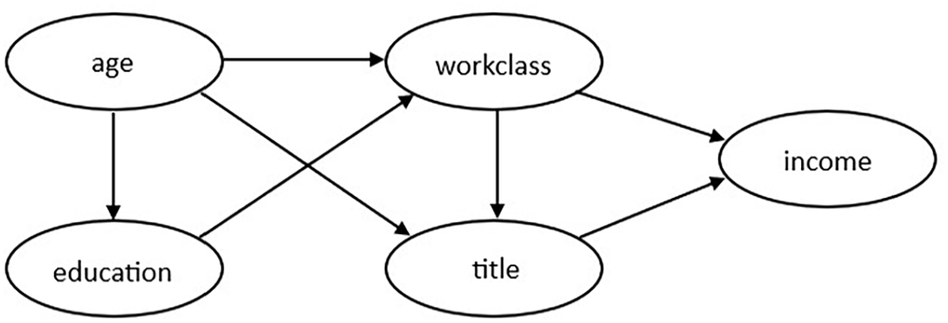
Bayesian network over five attributes, as shown in Zhang et al. (2017).
The Bayesian network allows approximation of the distribution using a set of low-dimensional marginals. Noise is injected into each marginal to ensure differential privacy, and the noisy marginals and Bayesian network are then used to construct an approximation of the data distribution. PrivBayes then draws samples from this to generate a synthetic dataset. DataSynthesizer, developed by Ping et al. (2017), is a Python package that implements a version of PrivBayes. Data–Synthesizer also allows the use of
Differential Privacy (DP; Dwork and Roth 2014) is a definition of privacy based on a quantifiable guarantee when releasing data. An algorithm (or mechanism) is fully differentially private if, from the output alone, it is not possible to ascertain whether data from a specific individual was included in the computation. Satisfying DP is therefore a statement about the algorithm (or mechanism), rather than the data (or output) itself. In order to satisfy
In practical work, National statistical agencies have released synthetic versions of microdata using forms of multiple imputation. The United States Census Bureau released a synthetic version of the Longitudinal Business Database (SynLBD; Kinney et al. 2011), the Survey of Income and Program Participation (SIPP) Synthetic Beta (Benedetto et al. 2018), and the OnTheMap application (Machanavajjhala et al. 2008). Whilst government organizations have not so far released synthetic microdata created using deep learning methods, research in this area is ongoing (e.g., Kaloskampis et al. (2020) and Joshi (2019)).
2.3. Deep Learning for Categorical Data Synthesis
Deep learning (LeCun et al. 2015) is a subset of the broader field of ML and uses artificial neural networks to learn models from data. Neural networks (NNs) are made up of a series of stacked layers of neurons joined by weighted connections (the term “deep” refers to the number of hidden layers; a “shallow” NN may contain only one or two layers). In general, a NN is trained and learns iteratively by backpropagating the loss or error, through the network and adjusting the weights to reach an optimal solution. As described by LeCun et al. (2015), deep learning methods can discover the underlying structure in complex, high-dimensional data and have been responsible for performance improvements in areas such as speech recognition, image recognition, object detection, natural language understanding and genomics.
GANs (Goodfellow et al. 2014) and VAE (Kingma and Welling 2014) are generative methods that use NNs to model the distribution of the data. Broadly, the methods aim to probabilistically describe how a dataset is generated, therefore allowing new data to be generated by sampling from the model. A typical GAN, as shown in Figure 2, trains two NN models: a generative model that captures the data distribution and generates new data samples, and a discriminative model that aims to determine whether a sample is from the model distribution or the data distribution. The models are trained together in an adversarial zero-sum game framework (i.e., one’s gain is the other’s loss), such that the generator goal is to produce data samples that fool the discriminator into believing they are real and the discriminator goal is to determine which samples are real and which are fake. Training is iterative, using backpropagation (Rumelhart et al. 1986) to feed the errors (or gradient of the loss function) back through the layers of each NN in order to adjust the weights for the next round of training. Ideally during training both models improve over time, with the goal being a situation where the discriminator can no longer distinguish which data is real or fake.
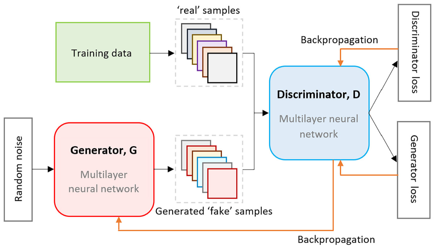
Structure of a typical GAN (Generative Adversarial Network).
GANs have many adjustable parameters—from the number of layers in each NN (and the number of nodes in each layer), to the loss function (to calculate the distance between the distribution of the real data and the generated data, e.g., mean squared error, Wasserstein loss), to the learning rate (controlling how much the weights are updated during backpropagation), to the number of epochs (or iterations) to train for—with so many options, it can be difficult to determine the optimal setup. It can also be challenging to optimize a GAN, in that it can be difficult to balance the training of both models (generator and discriminator); if they do not learn at a similar rate then the feedback may not be useful. GANs can be susceptible to issues such as vanishing gradients (where the discriminator does not feedback enough information for the generator to learn), mode collapse (e.g., the generator finds a small number of samples that fool the discriminator and only produces those, leading to the gradient of the loss function to collapse to near 0), and failure to converge.
VAE (Kingma and Welling 2014) consist of two linked but independently parameterized NN models, which support each other: the encoder (or recognition) model and the decoder (or generative model; Kingma and Welling 2019). The encoder compresses the original data into a latent distribution, then the decoder tries to transform the distribution back into a meaningful representation of the original data. The objective of VAE training is to minimize the error in this process. VAE can be used to generate synthetic data because it can capture the lower-dimensional dependencies in the original dataset and then produce new data which is similar, but not the same, as the original data (Wan et al. 2017). However, as detailed by Huang et al. (2018) and Wang et al. (2020) at least in terms of image production, VAE tend to produce images that lack detail, whereas GANs can usually generate sharper images (albeit they may face greater challenges in terms of training stability).
VAEs have been used predominantly for augmentation or synthesis of image data (e.g., Laptev et al. (2021), Turénko et al. (2020), and Wan et al. (2017)). However, these usages focus on homogeneous data, and as noted by Ma et al. (2020) and Nazabal et al. (2020), vanilla VAEs (i.e., those corresponding to Kingma and Welling’s (2014) original description) generally perform poorly on mixed type data and/or data with missing values. This is because data of mixed type (e.g., categorical, continuous) may be modeled poorly if all variables are treated in the same way (regardless of type) rather than adapted to optimize the different types. To counter this Ma et al. (2020) proposed the Variational Auto-Encoder (VAEM) for heterogeneous mixed type data, which trains an individual VAE for each variable and then trains a dependency network to connect them all (which models the inter-variable statistical dependencies), and Nazabal et al. (2020) proposed a similar framework but trains the VAEs jointly as opposed to in two stages.
Like VAEs, GANs have been used extensively for image generation and tend to deal with numerical, homogeneous data; they must be adapted in order to be able to handle categorical data. Several studies have done this by adapting the GAN architecture, these adaptations are often referred to as tabular GANs (e.g., Camino et al. (2018), Park et al. (2018), Zhao et al. (2021), and Chen et al. (2019)). Conditional Tabular GAN (CTGAN), developed by Xu et al. (2019) uses “mode-specific normalization” to overcome non-Gaussian and multimodal distribution problems, and employs oversampling methods (“training-by-sampling”) and a conditional generator to handle class imbalance in the categorical variables. Briefly, the conditional generator can explicitly condition on specific categories of a variable: if a variable has a category that covers the majority of cases (say
3. Research Design
In this study, the performance of four state-of-the-art data synthesis software implementations (synthpop, DataSynthesizer, CTGAN, TVAE) on census microdata was compared by systematically exploring the effect of different parameter settings on the disclosure risk and utility of the resulting synthetic data. Each synthesizer was tested on four different census microdata sets (Canada, Fiji, Rwanda, UK). For each individual parameter setting, five models were generated (with different random seeds) each producing one dataset. For each of these groups of five datasets, the means of the disclosure and utility metrics (described in Subsections 3.3 and 3.4) were calculated. The following section describes the synthesizers, parameter selection, census datasets, and the evaluation metrics. Figure 3 contains an overview of the workflow from preparation to evaluation.
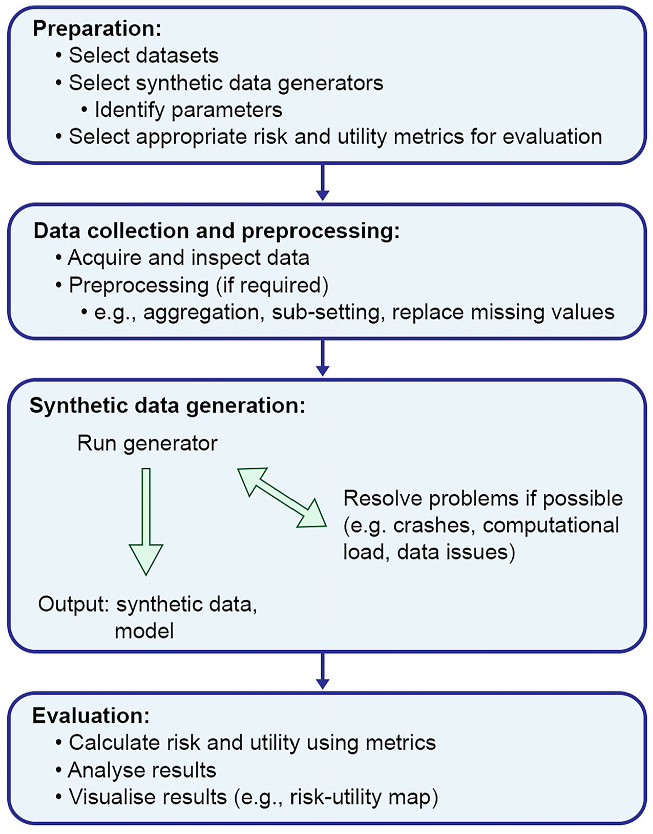
Analytical pipeline adopted in this study.
3.1. System and Parameter Selection
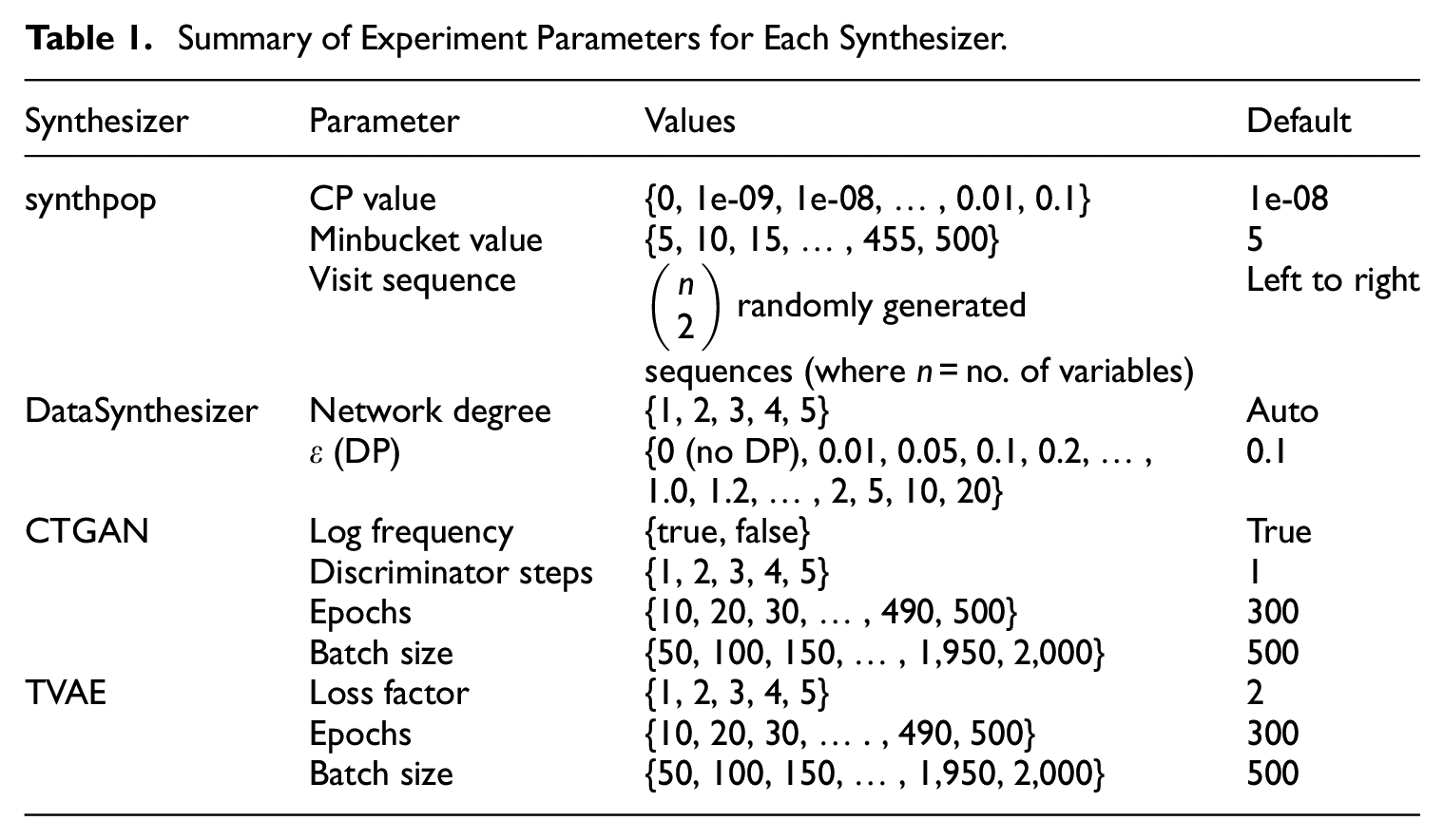
The data synthesis software implementations used were synthpop (Nowok et al. 2016), DataSynthesizer (Ping et al. 2017), CTGAN and TVAE (both proposed by Xu et al. 2019). These were selected as they are established, open-source implementations that should produce good quality data. Initial pilot experiments also included TableGAN (Park et al. 2018), however this was found to perform badly (falling into mode collapse) and it was therefore not included in further experiments. For each experiment, one parameter of interest was varied while using the default parameters settings for others. We obtained default parameter settings from the source papers, code repositories, and documentation published by the authors. We experiment only with parameters that were designed to be changeable, that is, we do not edit the source code of any of the synthesizers. Table 1 summarizes the parameters experimented with, whilst the following section describes them in more detail.
Summary of Experiment Parameters for Each Synthesizer.
3.1.1. synthpop
Version 1.6-0 of synthpop was used for all experiments. Default parameter settings were obtained from the package documentation (Nowok et al. 2022). As described in Section 2.2, synthpop (using the default method of CART) allows the sequence order of the variables (called the visit sequence) to be set by the user, by default the ordering is set such that the columns are read from left to right. The visit sequence experiments attempt to determine the importance of ordering. The census microdata used for these experiments is predominantly categorical, with some variables containing many (>20) categories. It is known that the performance of synthpop can become very slow as the trees become more complex (which happens when variables contain many categories); to deal with this, Raab et al. (2017) suggest moving variables with many categories to the end of the sequence. The visit sequence for the other two experiments were therefore set so that variables were ordered by the minimum to maximum number of categories, with numerical variables first (and a tie decided by alphabetical ordering) in order to minimize overall complexity. Experiments were performed with three parameter settings:
• Complexity Parameter (CP): The CP value, between 0 and 1, controls tree size. Smaller values grow larger, more complex trees (a value of zero grows a full tree) whereas larger values grow less complex trees (e.g., with fewer splits).
• Minbucket Size: The minbucket value controls the minimum size of (or minimum number of observations in) the final node of each tree, which may help to control disclosure risk.
• Visit Sequence: The order in which the variables are processed. Whilst for compute time it may be optimal to place the categorical variables with many levels at the end of the sequence, this may not be optimal for data quality. It was not feasible to try every possible visit sequence combination (e.g., the number of combinations for the UK dataset, with fifteen variables, would be greater than a trillion), for each census dataset, sequences were generated such that all possible combinations of the variables in the first two places (e.g., {1,2}, {1,3}, {1,4}, … , {15,14}, where there are fifteen variables) were used, then the remaining were generated randomly. Randomly generated sequences were used, as the focus was to demonstrate whether the ordering affects the results, rather than to specify particular orderings which would only be valid for those particular datasets. In practice, those generating synthetic data should choose visit sequences strategically.
3.1.2. DataSynthesizer
Version 0.1.9 of DataSynthesizer (described in Section 2.2) was used for all experiments in Correlated Attribute mode (which implements the PrivBayes (Zhang et al. 2017) algorithm). Parameter details were obtained from the code repository (DataResponsibly 2023). Experiments were performed with two settings:
• Differential Privacy (DP): DP is controlled by the
• Network Degree: For the degree of the Bayesian network, which is the maximum number of parents of a Bayesian network node (higher values increase complexity), values of 1, 2, 3, 4, and 5 were used. Using the default value (0) for this means the algorithm automatically calculates the degree.
3.1.3. CTGAN
Version 0.4.3 of CTGAN was used for all experiments. CTGAN as described in Subsection 2.3, is a Conditional GAN implemented in Python. Information on the default parameters was obtained from Xu et al. (2019), the code repository (sdv-dev 2024a) and website documentation (SDV 2022a). As noted in Subsection 2.3, GANs tend to have many settable parameters, to decrease complexity we chose not to change the architecture of the GAN (e.g., changing the number and size of layers in the generator and discriminator), instead concentrating on parameters that could affect the performance of CTGAN as is. Experiments were performed on the following parameters:
• Log Frequency (LF): As described in Subsection 2.3 CTGAN uses a conditional generator and “training-by-sampling” to deal with imbalanced classes in the categorical variables (in a traditional GAN, minority classes may simply be ignored if the GAN does not account for this). CTGAN samples the data during training and counts the frequency of the category levels. The LF parameter controls whether (true) or not (false) the log frequency of categorical levels is used in conditional sampling. It therefore affects how the model processes the frequencies of categorical values. The documentation states that changing this to False could in some cases improve performance.
• Discriminator Steps: The number of discriminator updates performed for each generator update.
• Number of Epochs: The number of cycles for which the model trains.
• Batch Size: The number of records in each batch of data used whilst training the model.
3.1.4. TVAE
Version 0.12.1 of the sdv Python package containing TVAE was used for all experiments. TVAE as described in Subsection 2.3, is a Variational Autoencoder implemented in Python. As with CTGAN to decrease complexity we chose not to change the architecture of the model (e.g., changing the number and size of layers in the NNs), instead concentrating on parameters that could affect the performance of TVAE as is. Default parameter values were used (obtained from the code repository (sdv-dev 2024b) and code documentation (SDV 2022b) whilst varying one of the following parameters:
• Number of epochs: The number of cycles for which the model trains.
• Batch size: The number of records in each batch of data used whilst training the model.
• Loss factor: Simply stated, the encoder NN of TVAE maps a lower-dimensional representation of the original data, and the decoder NN attempts to reconstruct the original data from that representation. The model is trained to minimize the reconstruction loss (or error), that is, the difference between the original data distribution and the data reconstructed by the decoder. The overall combined loss for the model is the sum of two parts, the reconstruction loss and Kullback-Liebler divergence loss. The loss factor parameter scales (or weights) the reconstruction loss and therefore affects the combined loss result. This is used to calculate the gradients in the backpropagation step and affects how the model learns (if the gradients are too small or too large the model may stop learning). The default loss factor value is 2.
3.2. Data
Census microdata from four different countries, that is, Canada, Fiji, and Rwanda (obtained from IPUMS (Minnesota Population Center 2020)) and UK (obtained from ONS (Office for National Statistics, Census Division, University of Manchester, Cathie Marsh Centre for Census and Survey Research 2013)) were used, with each dataset from a different continent to optimize diversity. Each dataset is a sample of individual records, pertaining to both adults and children. The variables include demographic information, such as age, sex, and marital status (i.e., variables that are often considered key identifiers) and a broad selection of variables pertaining to employment, education, ethnicity, family, etc. The exact set of variables was different for each country, reflecting differences in culture and data collection processes, but the subsets analyzed here contain a common core set of variables (e.g., age sex and marital status) and other variables related to the same overall themes (such as employment and education). The purpose of using multiple datasets was not to directly compare the countries, but rather to determine whether any patterns or relationships uncovered during the experiments were replicated on similar (but not identical) datasets.
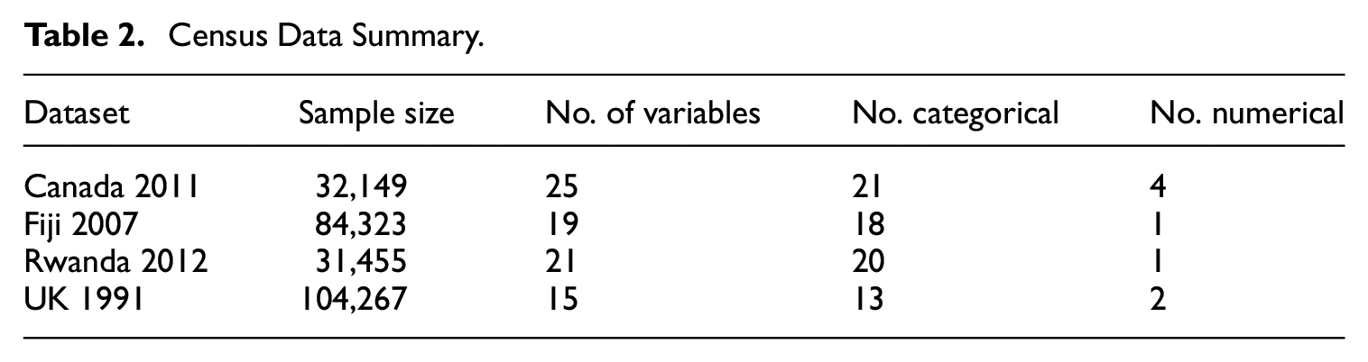
Each dataset contained categorical variables with many categories, numerical variables and variables with imbalanced distributions. Whilst there is a temptation to aggregate variables with many categories into fewer categories (which computationally might make synthesis simpler), the aim of these experiments was to attempt to capture the entire distribution of the data (whilst also determining the limitations of the synthesizers), therefore no variable was aggregated. However, three of the datasets (UK, Canada, and Rwanda) were sub-setted on a randomly selected geographical region to reduce computational load and also to naturally reduce the categories for some of the variables (the exception was Fiji, for which the entire sample was used). For all datasets (synthetic or original, the same approach was adopted for both), missing values were retained. That is, no values were imputed and where required for analysis missing values constituted an extra category (for categorical data). Table 2 describes the data used for the experiments in terms of sample size and features; more detail can be found in Appendix A.
Census Data Summary.
For each of the four datasets, we created a “baseline” dataset containing the same number of records and variables as the original, with each variable randomly drawn from the univariate probability distributions of the original data (independently of the other variables). This represents the minimal level of meaningful utility, as the univariate distributions of each variable in the baseline datasets were similar to the original but the relationships between the variables in the original data were not replicated. The rationale for these datasets is that since aggregate univariate census statistics are routinely publicly available, a baseline dataset like this could therefore be constructed. To ensure robustness of the results, 1,000 baseline datasets were generated for each country. The utility and disclosure metrics (described in the next section) were applied to these (as they were to the synthesized data, by comparing to the original dataset) and the mean calculated to produce overall baseline utility and disclosure risk scores for each country. “Random” datasets were also generated, in the same way, but using uniform instead of the observed unvariate distributions (e.g., if a variable had two categories, they would be split 50/50). The baseline and random data points are plotted on the R-U map for each experiment result.
3.3. Measuring Disclosure Risk Using TCAP
For the experiments within this article, we refer to the attribute disclosure risk simply as the disclosure risk, since this is the main form of disclosure risk associated with synthetic data (as discussed in Subsection 2.1). Elliot (2014) and Taub et al. (2018) introduced a measure for the disclosure risk of synthetic data called the Correct Attribution Probability (CAP) score. The disclosure risk is calculated using an adaptation used by Taub and Elliot (2019) called the Targeted Correct Attribution Probability (TCAP). TCAP is based on a scenario whereby we assume that an intruder has partial knowledge about a particular individual and they wish to infer the value of a sensitive variable (the target) for that individual. Specifically we assume that they:
• know the individual is in the original dataset (that was used to generate the synthetic data)
• know the individuals’ values for some of the variables in the dataset (the keys).
• match the known values against the synthetic dataset
The TCAP metric is then the probability that those matched records (on the keys) yield a correct value for the target variable (i.e., that the intruder makes a correct attribution inference). These are strong assumptions, which have the benefit of then dominating most other scenarios, with the one possible exception being a membership inference attack. However, for census microdata, because they are a random sample of a country’s population, membership is not itself informative; unlike, for example, membership of a dataset of people that have a particular illness where membership itself is a form of attribute disclosure.
The TCAP measure is used because it is easily computable across all methods (since it simply compares matching records from the original and synthetic datasets), which is a benefit over other measures such as that proposed by Hu et al. (2014) which could be computationally intractable for larger datasets and relies on the very strong assumption that the intruder knows every case but one.
Following Taub and Elliot (2019), TCAP is calculated as follows: define

Likewise,

The Within Equivalence Class Attribution Probability (WEAP) score for the synthetic dataset is then calculated. The WEAP score for the record indexed j is the empirical probability of its target variables given its key variables
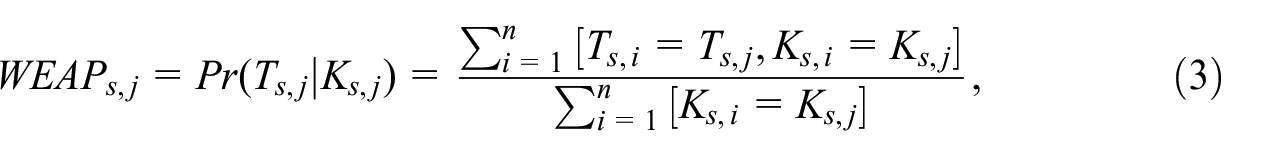
where the square brackets are Iverson brackets,
The TCAP for record j based on a corresponding original dataset do is the same empirical, conditional probability but derived from do,
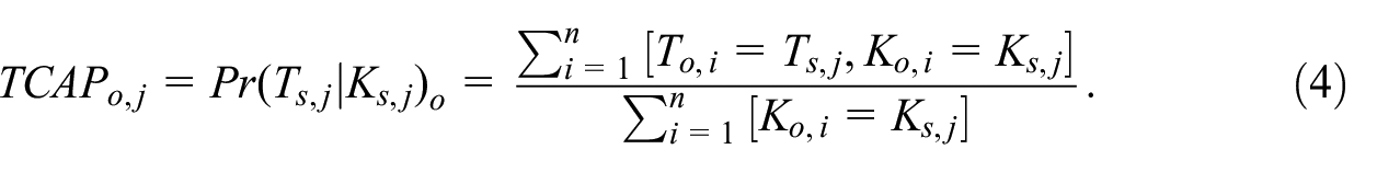
For any record in the synthetic dataset for which there is no corresponding record in the original dataset with the same key variable values, the denominator in Equation (4) will be zero and the TCAP is therefore undefined.
TCAP has a value between 0 and 1; a low value would indicate that the synthetic dataset carries little risk of disclosure, whereas a TCAP score close to 1 indicates a higher risk. With the same rationale as with the baseline datasets, a baseline risk value can be calculated (essentially the probability of the intruder being correct if they drew randomly from the univariate distribution of the target variable). The TCAP baseline is included in all of the R-U plots.
For each census dataset, three targets and six key variables were used, and the corresponding TCAP scores calculated for sets of 3, 4, 5, and 6 keys (based on the standard key variable sets produced by Elliot et al. (2020)). The overall mean of the TCAP scores was then calculated as the overall disclosure risk score. Where possible, the selected key/target variables were consistent across each country. Full details of the target and key variables are in Appendix B.
3.4. Evaluating Utility
Following Taub et al. (2020) and Little et al. (2021), the utility of the synthetic data was assessed with a basket of measures using confidence interval overlap (CIO), ratios of counts (ROC), and propensity score mean squared error (pMSE) approaches. The CIO is considered a specific (or narrow) utility measure whereas the pMSE is considered a general (or broad) measure. Specific utility measures compare the difference between results for specific analyses using both the original and synthetic data, whereas general measures provide summaries of the differences between the distributions of the original and synthetic data (Snoke et al. 2018). Including the different types of measures in this basket approach aims to provide a more complete picture of the utility than any single measure could.
The CIO (using 95% confidence intervals) was used for the coefficients from regression models. The CIO, proposed by Karr et al. (2006), is defined as:
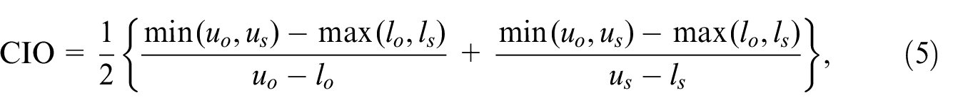
where
Frequency tables and cross-tabulations were evaluated using the ROC, which is calculated by taking the ratio of the synthetic and original data estimates (where the smaller is divided by the larger one). Thus, given two corresponding estimates (e.g., the number of records with sex = female and age = 29 in the original dataset, compared to the number in the synthetic dataset), where
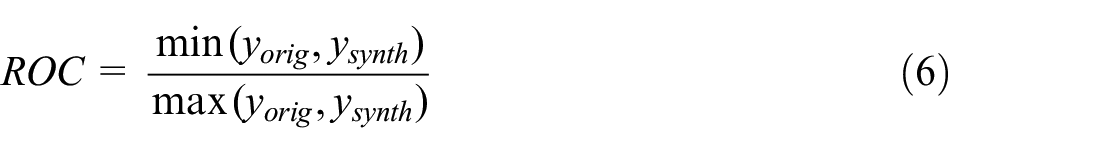
If
The pMSE, developed by Woo et al. (2009) and Snoke et al. (2018), is a measure of data utility designed to determine how easy it is to discern between two datasets based upon a classifier. It is calculated by merging the original and synthetic datasets and creating a variable
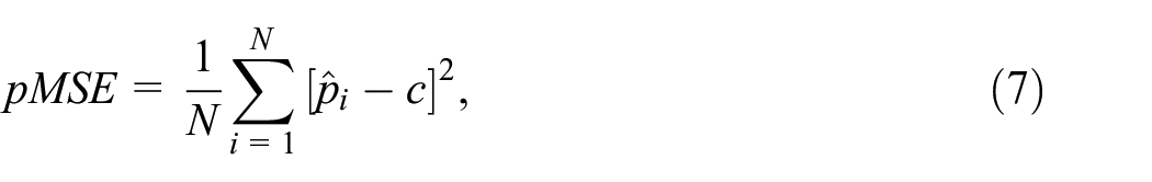
where
As suggested by Bowen and Snoke (2021) and Raab et al. (2021), the pMSE for this study is calculated using CART (rather than logistic regression) as it can model more complex relationships in the data. Following Bowen and Snoke (2021), the null mean pMSE was estimated using the original data. To do this twice the number of rows was bootstrapped from the original data with labels of 0 assigned to half and 1 to the other half, the pMSE was calculated, and this was repeated one hundred times; the average value is the null pMSE which was then used to calculate the pMSE-ratio. To align with the other utility measures used for this study (where a score close to 1 indicates high utility), the pMSE-ratio was scaled to between 0 and 1 (by dividing by the maximum score across all experiments performed on that census dataset, and then subtracting from 1), with a higher score meaning higher utility.
To create an overall utility score for comparing against the overall disclosure risk score (TCAP), the mean of the ROC scores, the CIO, and the pMSE-ratio was calculated—a score closer to zero would indicate lower utility whereas a score closer to 1 would indicate higher utility. Each of the measures (bivariate ROC, trivariate ROC, CIO, and pMSE-ratio) were given equal weight when calculating the mean, an avenue for future research would be to experiment with different weightings, or a multi-objective approach.
4. Results
For each experiment, we generated fully synthetic datasets the same size as the original. No post-processing of the data was performed (aside from correcting some of the DataSynthesizer output for the Canada data, see Subsection 4.3.1). To account for any problems with computational load, all models were given forty-eight hours to run before they were terminated. In the event that a model crashed, it would be given one more run before discarding.
The results obtained with the default parameters are presented first, then grouped by method followed by an overall comparison. Each of the plots of the R-U map include a line marking the TCAP baseline. They also contain a point representing the original data (necessarily with utility = 1 and risk (TCAP) = 1) and a point representing the baseline and random datasets for that country (discussed in Subsection 3.2). The baseline utility and disclosure risk scores for each country are contained in Appendix D. Whilst not included in the plots, we refer in the analysis to a notional R-U gradient—this is the diagonal line between the original data point and the origin. It is not plotted because it is arbitrary and dependent upon the particular risk and utility measures used, but it can provide a simple rule of thumb—points to the right of this line could indicate that the utility loss is lower than the reduction in risk.
4.1. Default Parameters
Figure 4 plots the results using the default parameter settings of the four data synthesizers, indicating what is possible without changing parameters. The plot illustrates that, irrespective of the particular dataset, synthpop produced data with the highest utility compared to the other synthesizers, albeit with high risk. synthpop was the only synthesizer with results to the right of the notional R-U gradient (not plotted, the diagonal line between the origin and original data point). DataSynthesizer had consistently the lowest utility, close to data that was randomly generated (yet with higher risk). CTGAN and TVAE produced results that occupied similar areas on the R-U map for all but the Canada data. This may be because the distribution of the Canada data was more difficult to learn for those synthesizers; the Canada data had more variables (25) than any of the other datasets which may have been a factor.
R-U plots of the results for each synthesizer when using default parameters (each point is the mean of 20 runs of the particular synthesizer, standard error <0.017 for all measures), for each census dataset.
4.2. synthpop
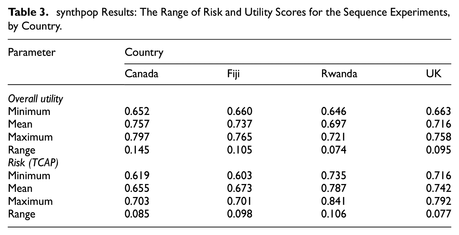
To illustrate how the overall utility and risk scores are calculated an example detailing the individual utility metrics and TCAP results, using the synthpop CP parameter experiment, is contained in Appendix E. Figure 5 plots the results for each of the three parameter experiments for the UK Census data. Individual plots for each experiment and country are contained in Appendix F. The results visualized in Figure 5 show that changing the parameters has a bigger effect on utility than risk, and the CP value had the greatest effect on risk and utility (producing a wider range of results) compared to the other parameters. Utility and risk reduced as the minbucket value increased, therefore it is possible that setting this slightly higher (up to about 50) than the default value of 5 might allow some fine-tuning whereby risk could be reduced without too much utility loss. Simply changing the order of the visit sequence, which is a setting that could be overlooked, can make a difference to both utility and risk as shown in Table 3, which lists the range of results in terms of risk and utility for the visit sequence experiments.
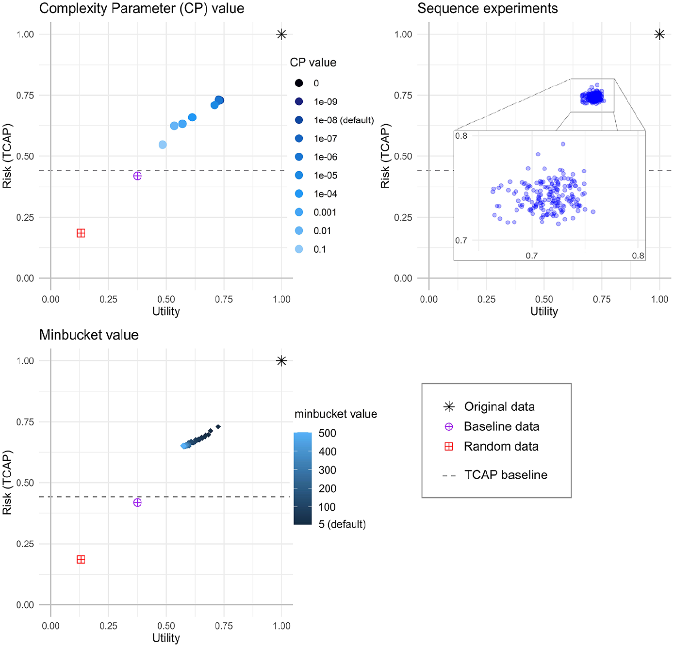
R-U plots of the synthpop results (each point is the mean of 5 runs of the synthesizer, standard error <0.007 for all measures) for UK 1991 Census data.
synthpop Results: The Range of Risk and Utility Scores for the Sequence Experiments, by Country.
4.2.1. Experimental Observations
synthpop was simple to use, with good documentation. It was the quickest to run, with average running time (using default parameter settings) ranging from 1.5 minutes (for the Rwanda data) to 31 minutes (for the Fiji data). However, variables with many categories did prove to be a problem, in that experiments where those variables were placed nearer the beginning of the visit sequence did not manage to complete the run (they were given forty-eight hours to complete and then terminated), and the experiments had to be adapted to deal with this. For the UK, Canada and Rwanda data, the birthplace variable (having >36 categories) had to be affixed to the end of the visit sequence (and therefore excluded as a predictor). For the Fiji data, four variables (each with >28 categories) were excluded as predictors. These changes allowed the models to run and results to be generated. However, if the inclusion of such variables is particularly important to an analysis, then one might consider aggregation, stratification, or the use of a different method.
4.3. DataSynthesizer
Figure 6 plots the results for the two parameter experiments for the UK Census data. Individual plots for each experiment and country are contained in Appendix G. The majority of experiments produced data with low utility, below the baseline—only where DP was turned off (or also
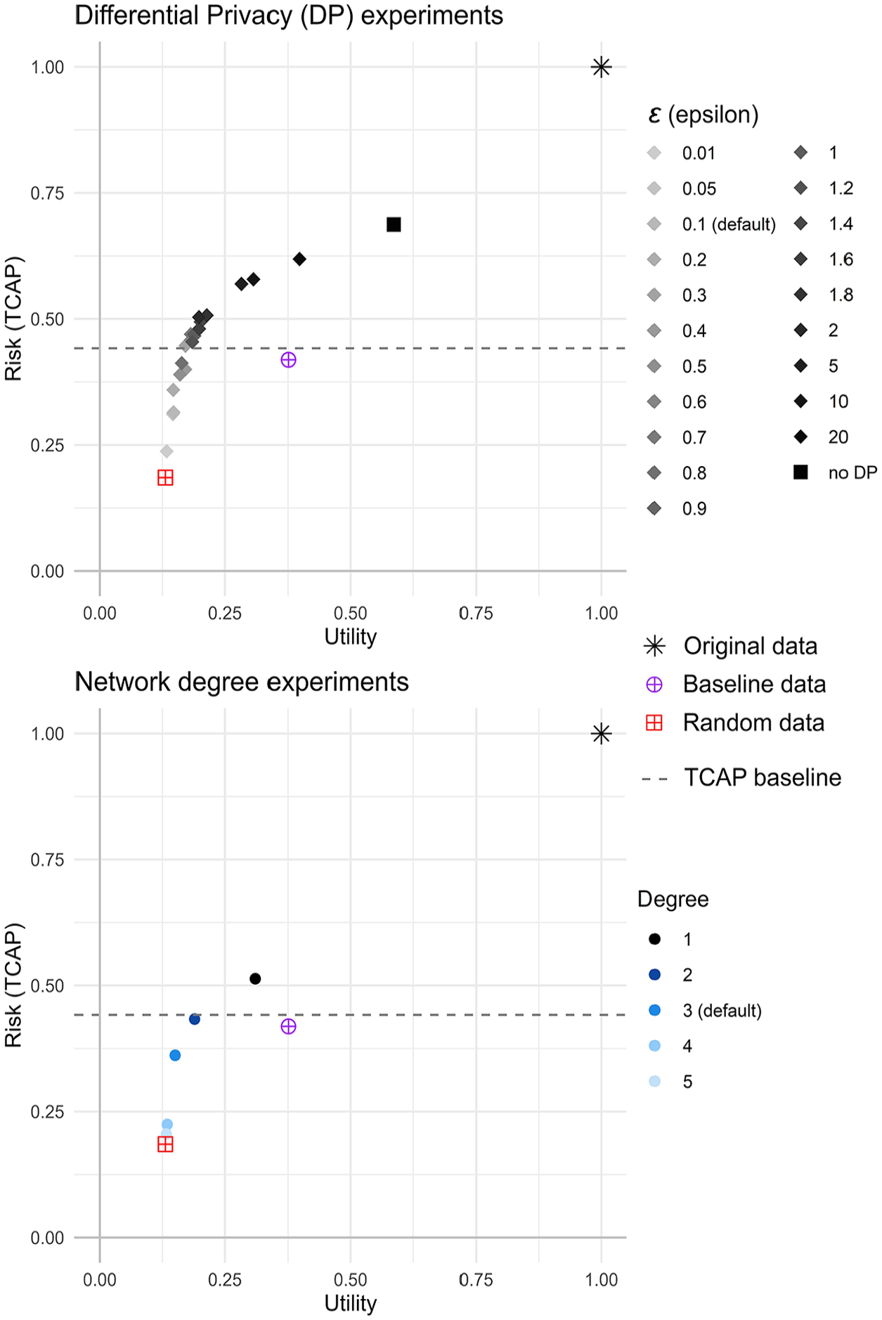
R-U plots of the DataSynthesizer results (each point is the mean of 5 runs of the synthesizer, standard error <0.041 for all measures) for UK 1991 Census data.
4.3.1. Experimental Observations
DataSynthesizer was typically quicker to run than the deep learning synthesizers (CTGAN and TVAE) but slower than synthpop. The average running time (using default parameter settings) ranged from thirty-six minutes (for the UK data) to eighty-nine minutes (for the Fiji data). The DP experiments attempted to use the default value for the network degree (0, which would automatically calculate it), however this resulted in the Rwanda and Canada DP experiments not completing due to excessive computational load. The PrivBayes algorithm was designed to use low-degree Bayesian networks to approximate high-dimensional data, therefore the degree value should be low (Zhang et al. 2017); a value above 5 introduces high computational load. Whilst for the UK and Fiji data the degree value was automatically calculated as 3, for Rwanda it was automatically calculated as 10, and for Canada as 12, which meant the models for Canada and Rwanda did not complete (the models were given forty-eight hours before they were terminated). To allow results to be collected for those countries, the degree value was set at 3. It should also be noted that no results were returned for the Fiji network degree experiments when using a network degree value of 5; this was because the models produced were so large that the computational load became too high (this is likely because the Fiji data was complex, with five out of the nineteen variables containing >20 categories). DataSynthesizer also occasionally produced inconsistent errors, which appeared to stem from misidentifying data types (identifying categorical text as a social security id type); this meant that models occasionally needed to be rerun (if the model crashed, it was given one more run), and for some experiments the Canadian data required post-processing as one of the variable categories was different (although still identifiable) to the original data.
4.4. CTGAN
Figure 7 plots the results for the four parameter experiments for the UK Census data. Individual plots for each experiment and country are contained in Appendix H. The number of epochs had the greatest effect on risk and utility; utility and risk increased as the number of epochs increased (in general utility and risk rose quite quickly up to about fifty epochs, then utility tended to rise very slowly whereas risk remained fairly steady). The other three parameter settings had a smaller effect: there was no consistent pattern across the different census datasets for the log frequency setting or the batch size; and a higher number of discriminator steps resulted in a very small increase in utility.
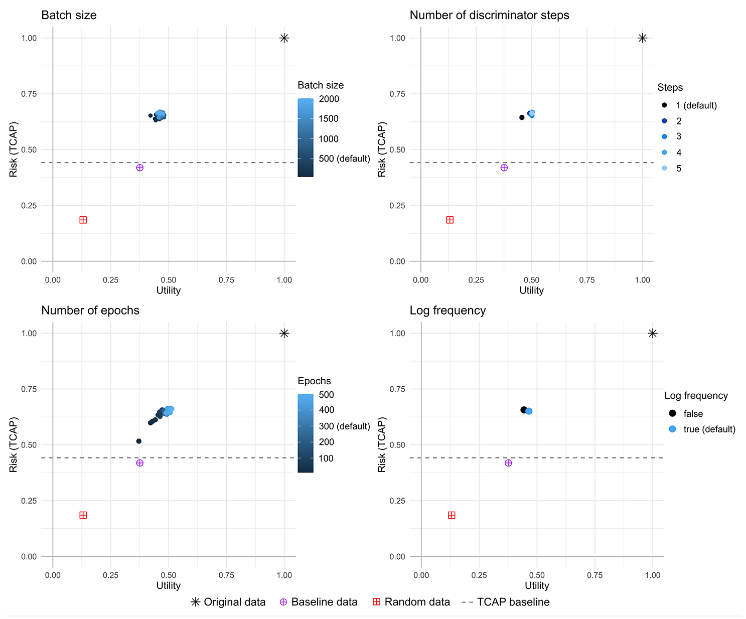
R-U plots of the CTGAN results (each point is the mean of 5 runs of the synthesizer, standard error <0.017 for all measures) for UK 1991 Census data.
4.4.1. Experimental Observations
CTGAN was relatively simple to use, with good documentation and no problems were encountered when running the experiments. CTGAN took the longest to run, with average running time (using default parameter settings) ranging from 120 minutes (for the Rwanda data) to 504 minutes (for the Fiji data). As might be expected the running time was longer the more epochs were used, or the smaller the batch size.
4.5. TVAE
Figure 8 plots the results for the three parameter experiments for the UK Census data. Individual plots for each experiment and country are contained in Appendix I. All three parameter settings had a noticeable effect on the utility and risk. As the number of epochs was increased the utility also did, and in general the risk decreased. Both these effects leveled out as the epochs increased. The batch size had the most effect on the utility of the data, with a smaller batch size resulting in higher utility, and for all datasets other than Fiji the risk was fairly flat. A value of 1 for the loss factor resulted in data with highest risk and lowest utility, whereas higher values had lower risk and higher utility. In general, a loss factor value higher than the default of 2 produces data with higher utility and lower risk. For the epochs, generally using more than the default of three hundred results in a small increase in utility with little effect on the risk. And for the batch size, a value higher than the default of 50, between about 100 and 200 produces data with slightly higher utility and comparable risk. For some of the experiments TVAE exhibited the unexpected result of reducing risk and increasing utility; it is possible this is related to TVAE using the original data as part of the training process (the encoder produces a lower-dimensional representation of the original data). However, these experiments still tended to display higher risk (compared to the other synthesizers), and relatively low utility, which is generally not desirable.
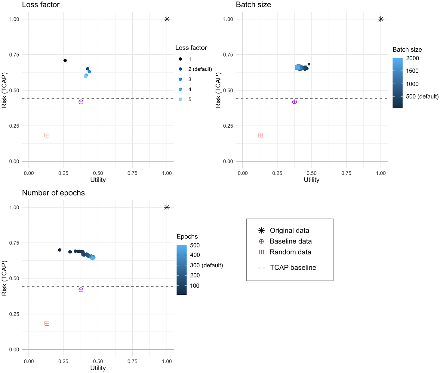
R-U plots of the TVAE results (each point is the mean of 5 runs of the synthesizer, standard error <0.020 for all measures) for UK 1991 Census data.
4.5.1. Experimental Observations
TVAE was relatively simple to use, with good documentation and no problems were encountered when running the experiments. Average running time (using default parameter settings) ranged from twenty-four minutes (for the Canada data) to ninety-four minutes (for the UK data).
4.6. Overall Performance
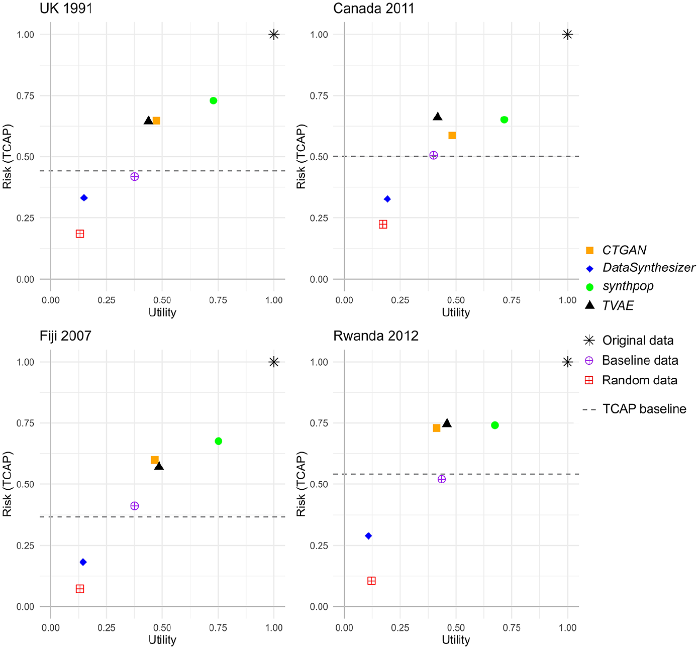
Figure 9 shows the results for all synthesizers and parameter experiments on one plot, by country. This is shown to highlight the different areas of the R-U map that each method covers, and to illustrate the range of results when parameters are changed from the default. Whilst there are differences between the census datasets, the overall pattern is similar across all four.
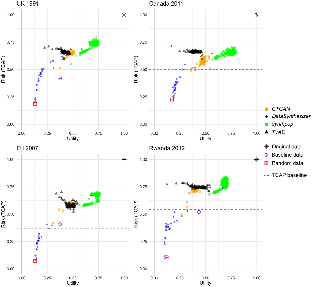
R-U plots of the results for all four synthesizers, by country. Each point is the mean of five runs of the synthesizer (with standard error <0.041 across all points).
Points that appear to the right of the notional R-U gradient (not plotted, a diagonal line between the origin and original data point) might be considered optimal in terms of the risk-utility trade-off, in that the utility is greater than the risk. The plot highlights that across all synthesizers synthpop produced most results to the right of the R-U gradient, whereas CTGAN and TVAE had none, and whilst DataSynthesizer had a few of these results all had utility close to that of a random dataset (and well below baseline).
4.6.1. “Best” Parameter Settings
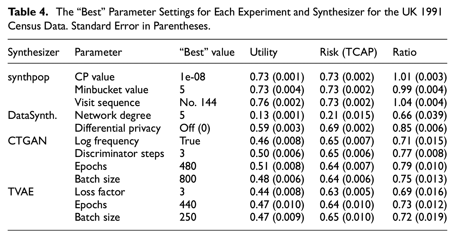
Here, we consider the “best” parameter setting (for each parameter) and the best overall setting for each synthesizer. The “best” result is subjective; different users may have different requirements in terms of setting an acceptable level of risk or utility. In this case, the “best” result is chosen as the one that has the highest utility/risk ratio (we recognize there are many other ways to specify “best”). Table 4 lists the “best” parameter setting for each experiment (only the UK data is shown for clarity). For instance, Table 4 shows that the “best” CP value for synthpop (on the UK data) was 1e-08. We can then look at each of the “best” parameter results for synthpop and see that the visit sequence parameter experiment (using sequence number 144, out of the 182 tried) resulted in the overall best result (the highest ratio across all of the synthpop parameter experiments considered together).
The “Best” Parameter Settings for Each Experiment and Synthesizer for the UK 1991 Census Data. Standard Error in Parentheses.
The overall “best” result for each method is plotted on the R-U map in Figure 10. Each “best” result is compared against the result using the default parameter settings. For all but DataSynthesizer the “best” and default points are fairly close together, and the “best” generally has higher utility and lower or comparable risk than the default. For the UK and Canada data the DataSynthesizer points are far apart, with the “best” having both higher utility and risk, for Fiji and Rwanda the “best” is comparable to the random dataset (the utility was so low for some of the experiments that it resulted in a very low risk score and hence the utility/risk ratio was high).
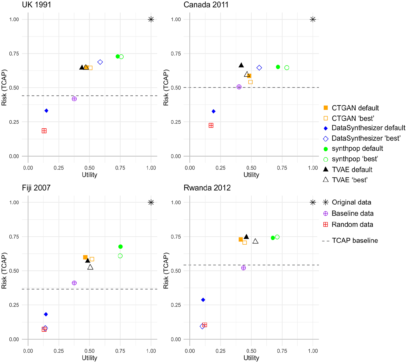
R-U plots of the “best” parameter setting compared to the default parameter setting, for all four synthesizers, by country.
Welch’s independent t-tests were calculated to compare experiments performed with the “best” setting (n = 5) to experiments performed with the default settings (n = 20). The discrepancy in size is because for each parameter setting an experiment was performed five times, so there were five results for each experiment, but in order to make sure that the estimates for the default were stable (because each experiment is compared to that) a larger value of 20 was chosen. T-tests were performed on the utility and risk (TCAP) scores separately. For example, the utility of the “best” experiments was compared to the utility of the experiments using the default settings, and the risk (TCAP) of the “best” experiments was compared against the risk of experiments using the default settings. For all but the Fiji TVAE experiment, the “best” settings demonstrated significantly better utility or risk (or both utility and risk for seven out of sixteen experiments) than the default at the 5% (α = .05) significance level.
Across all countries the “best” synthpop parameter setting came from the visit sequence parameter (i.e., changing the ordering of the data). For DataSynthesizer, changing the DP parameter gave the “best” results across all countries (simply turning it off for the UK and Canada data, or setting it so low (
5. Discussion
In terms of computational performance, modifications had to be made to some of the synthpop and DataSynthesizer experiments in order for them to return results. The CTGAN and TVAE synthesizers did not encounter any problems. For synthpop, the visit sequence experiments had to be modified such that variables with many categories were placed at the end of the sequence in order to reduce the computational load. As discussed, there are methods to deal with this (such as aggregation and stratifying), but if it is particularly important to a user that data with many categories are included completely then synthpop (using the default CART method) may not be the best choice. However, it should be noted that these experiments used the default CART synthesis implementation, and synthpop has the option of various alternative synthesis methods which may produce different results. Overall, synthpop was the only synthesizer that produced datasets that all had utility above the baseline; the trade-off was that the risk was also generally higher than for the other synthesizers.
In terms of privacy risk, DataSynthesizer was the only synthesizer that had a settable privacy parameter (
Of the two deep learning synthesizers, CTGAN showed the least effect when parameters were changed, with the number of epochs providing most change in risk and utility. Each of the three parameters of TVAE made a more noticeable difference. For all but the Canada data, the TVAE and CTGAN results tended to overlap on the R-U map, with TVAE generally having higher risk and comparable or slightly lower utility. CTGAN and TVAE in many cases had risk comparable to some of the synthpop datasets but much lower utility.
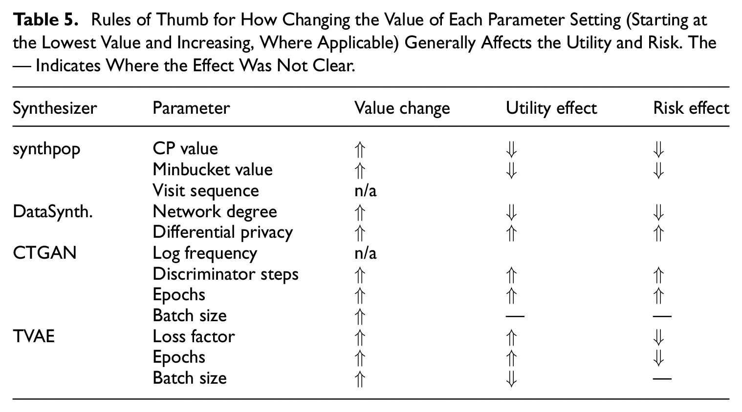
Table 5 lists a set of basic rules of thumb, that is, the general effect of increasing the value of each parameter setting. This aims to provide an overall view of the general trend observed during these experiments, and is applicable only to the four census datasets used in this study, different datasets may produce different results. The synthpop visit sequence experiment and CTGAN log frequency experiment are marked as n/a (not applicable) as their parameter values were not numeric, but a takeaway from the synthpop visit sequence experiments is that simply changing the ordering of the variables has the potential to provide some improvement in the utility or risk scores.
Rules of Thumb for How Changing the Value of Each Parameter Setting (Starting at the Lowest Value and Increasing, Where Applicable) Generally Affects the Utility and Risk. The — Indicates Where the Effect Was Not Clear.
It is worth noting that the census datasets used in these experiments may have been simplified via SDC techniques in order to allow their release. Therefore we do not know whether the experiments would replicate, or what effect it may have, to perform them on the underlying data—this would be an avenue for future work, if possible. It should also be considered that whilst we have systematically experimented with changing the parameter settings by differing one at a time (whilst all others were set at default), there may be combinations (including parameters that we did not experiment with) that provide “better” results. It is also noted that “better” is subjective, relying on what the individual user considers are acceptable levels of risk and utility, and that the choice of utility and risk measures also feeds into this.
Another point to raise is that the experiments conducted here were not constrained by practical situational requirements. In practice, a producer of synthetic data may have a maximum level of risk and/or a minimum level of utility that is considered acceptable. This will create a window on the overall R-U map that will be acceptable. In other cases—for example, the production of datasets for teaching purposes—there may be a requirement that the synthetic data reproduces specific analyses very well but requires only a broad similarity on many features (i.e., high use case specific utility but low fidelity data). The relationships between specific applications and the general study we report here is another potential area for future work.
6. Concluding Remarks
This study has examined four synthetic data generators and compared their performance in terms of risk and utility on four different census microdata sets. A greater understanding of these synthesizers can allow data owners to make informed decisions on the choice of method and parameter settings to use, and also provide a realistic view on what is achievable when generating synthetic data. The results show that for all synthesizers improvements can be made (increasing utility, decreasing risk) when different parameter settings are used, rather than simply using the default settings. The results also showed that the performance of the synthetic data generators was dependent upon the dataset as well as the parameter settings. Plotting the results on the R-U map highlighted the range of results that are available across the different synthesizers and indicate the type of results that each synthesizer might provide in terms of risk and utility. Future work would involve exploring a multi-objective (risk and utility) approach to synthetic microdata generation, whereby both could be optimized during the generation process.