Sage Journals: Discover world-class research

Abstract

It is widely appreciated that population forecasts are inherently uncertain. Researchers have responded by quantifying uncertainty using probabilistic forecasting methods. Yet despite several decades of development, probabilistic forecasts have gained little traction outside the academic sector. Therefore, this article suggests an alternative and simpler approach to estimating and communicating uncertainty which might be helpful for population forecast practitioners and users. Drawing on the naïve forecasts idea of Alho, it suggests creating “synthetic historical forecast errors” by running a regular deterministic projection model many times over recent decades. Then, borrowing from perishable food terminology, the “shelf life” of forecast variables, the number of years into the future the forecast is likely to remain “safe for consumption” (within a specified error tolerance), is estimated from the “historical” errors. The shelf lives are then applied to a current set of forecasts and presented in a simple manner in graphs and tables of forecasts using color-coding. The approach is illustrated through a case study of 2021-based population forecasts for Australia. It´s concluded that the approach offers a relatively straightforward way of estimating and communicating population forecast uncertainty.

Keywords

population forecasts shelf life forecast uncertainty Australia

1. Introduction

It is well known that population forecasts almost always differ to some extent from the population trends which eventually occur. Many studies have documented the extent, patterns, and determinants of forecast error (e.g., Bongaarts and Bulatao 2000; Gleditsch et al. 2021; Keilman 2001, 2008, 2019; Office for National Statistics (ONS) 2015; Rayer et al. 2009; Rees et al. 2001; Smith and Tayman 2003; Statistics New Zealand 2016; Wilson 2007; Wilson et al. 2018). As a general rule, error increases the further into the future the forecast extends and decreases with increasing population size (though there is little change in error above a certain size) (Tayman 2011). Errors at the youngest childhood ages and at the oldest ages, influenced considerably by births and deaths respectively, are often relatively large (Keilman 2019). Populations subject to high rates of migration often experience large errors in the young adult peak migration ages (Wilson 2012). Throughout this article I make the common definitional distinction between population forecasts, defined as predictions, and the broader term population projections, defined as the outcomes of calculations according to specified projection assumptions (Smith et al. 2013, 2–3). Forecasts always experience some degree of error; projections do not (unless there has been a calculation error).

Researchers have endeavored to both improve forecast accuracy and provide information on the uncertainty of forecasts. Over the last few decades, considerable effort has been devoted to improving the accuracy of demographic forecasts, especially for mortality (Ediev 2020; Janssen 2018). Many researchers have proposed methods aimed at improving fertility forecasting, but there is no single dominant method or approach and unfortunately fertility has proved stubbornly difficult to predict accurately (Bohk-Ewald et al. 2018; Gleditsch et al. 2021). Migration forecasting, both internal and international migration, generally presents the greatest challenge and is often subject to considerable amounts of uncertainty (Asoze et al. 2016; Bijak et al. 2019; de Valk et al. 2022; Fuchs et al. 2021). The coverage and quality of migration data is often lower than that for fertility and mortality, and migration trends can be highly volatile, being influenced by policy changes, the economic cycle, and major global events, all of which are very hard to predict. At the small area scale, migration can be heavily shaped by urban planning and the development of new suburbs. In internal migration projections research, much of the focus remains on model specification rather than parameter forecasting (e.g., Dion 2017; Vandresse 2016).

In terms of supplying information about uncertainty, the dominant approach has been to create probabilistic population forecasts. The stream of research on probabilistic methods has expanded hugely over the last three decades (Keilman 2020; Raftery and Ševčíková 2021), and in recent years increasingly sophisticated Bayesian approaches have been proposed (e.g., Billari et al. 2014; Graziani 2020; Raftery et al. 2012). Undoubtedly, research on probabilistic forecasting has contributed many important and valuable advances in demographic forecasting methodology. Importantly, there is also demand from users for information about forecast uncertainty. In an online survey and set of focus groups in Australia, forecast users expressed interest in receiving uncertainty information about population forecasts to aid decision-making, especially if it is communicated simply in plain language (Wilson and Shalley 2019).

Yet, there is a problem. Very few demographers in government and business who produce population forecasts use probabilistic methods. Many prefer high and low population scenarios, where the high-low difference is used to represent forecast uncertainty. But such high-low ranges are problematic because the scenarios are often based on arbitrary projection assumptions, there are no probabilities attached to the high-low intervals, and they contain statistical inconsistencies (Keilman et al. 2002). Statistics New Zealand (2022), Statistics Netherlands (2021), and Istat (2022) of Italy, along with the United Nations Population Division (2022), are among the few statistical agencies which currently publish probabilistic population forecasts. Some researchers have proposed simplified versions of probabilistic methods based on variant scenarios (e.g., Billari et al. 2012; Van Duin 2017) but use of these methods has been limited to date. The vast majority of government agencies and private sector organizations create forecasts with deterministic models. There are many possible reasons for this state of affairs. Probabilistic methods may be seen as highly complex, data-hungry, too demanding of staff time and budgets, or incompatible with other demographic forecasts produced by the same organization. Perhaps it is too difficult to decide between the many approaches and packages available for probabilistic forecasting. There may be a perception that users do not want probabilistic forecasts, or that they would be too difficult to communicate. Or perhaps there is concern that wide prediction intervals accompanying forecast variables will be interpreted by users as a sign of forecasting incompetence. Whatever the reasons, it is clear that probabilistic methods for forecasting population have been adopted by few outside the academic sector.

Therefore, I suggest an alternative, simpler approach to estimating and communicating population forecast uncertainty. It brings together Alho’s (1990) idea of estimating uncertainty from the errors of forecasts created for past periods, the concept of a “shelf life” borrowed from perishable food labeling (Wilson 2018), and traffic lights color-coding as a simple way of indicating reliability (Bijak et al. 2019). Primarily, the communication of uncertainty is achieved through visual means, taking the “less-is-more approach” recommended by Spiegelhalter et al. (2011) to appeal to a broad range of users. Importantly, my alternative approach does not require probabilistic modeling and can be implemented fairly easily with existing deterministic population projection models and existing input data. It is demonstrated using the example of 2021-based population forecasts for Australia prepared with a standard deterministic cohort-component model. Section 2 describes the approach and the data required to implement it. Section 3 presents population forecasts for Australia with the shelf life of the forecasts for selected population variables marked out on the graphs. The discussion and conclusions in Section 4 consider the strengths and weaknesses of the approach along with suggestions for further research.

2. Data and methods

2.1. Shelf Life Estimation

The approach to measuring forecast uncertainty draws on the ideas of Keyfitz (1981) and Stoto (1983), who estimated uncertainty from the errors of previously published forecasts, and also Alders et al. (2007) who made use of errors of published population projections produced by national statistical offices. My approach most closely follows that of Alho (1990), who generated a set of “naïve forecasts” of fertility for historical periods by assuming no change in fertility rates in the future. Calculating the deviations of these “forecasts” from observed values creates a distribution of “historical” errors. Rather than create naïve forecasts, the approach taken here is to prepare what might be termed “synthetic historical forecasts” in which the current projection model and assumption-setting approach is used to prepare forecasts for past periods. It produces the forecasts which would have been obtained if the current model and assumption-setting approach had been applied in the past.

Errors from many historical forecasts are used to calculate the number of years into the future the historical forecasts remained accurate (leaving aside for the moment how accuracy is defined). Borrowing terminology from perishable food labeling, this period of time is termed the “shelf life” of the forecast. The shelf life of food is the “period of time for which it remains safe and suitable for consumption, provided the food has been stored in accordance with any stated storage conditions” (New Zealand Ministry for Primary Industries 2016, 7). For population forecasts, it denotes the length of forecast horizon it is likely to remain sufficiently accurate for use. In fact, there are multiple shelf lives in any set of population forecasts because error varies according to the forecast variable, and will be different for the total population, age-sex-specific populations, proportions of the population in certain age groups, projected births, deaths and migration, and so on.

The shelf life of each population variable is then applied to the latest set of forecasts–both graphically and in tables–to provide users with a simple indication of how far into the future the forecasts should remain usable. It is based on the key assumption that the magnitude and patterns of error from the past will apply in the future. This is clearly an approximation, though several studies of forecasts made over many decades have found little or no improvement in forecast accuracy over time (e.g., Keilman 2008; Smith and Sincich 1988; Wilson 2007). However, the bias of forecasts–whether they tend to be too high or too low overall–is very difficult to predict (Tayman 2011). The approach described here incorporates only error, and not bias.

The process for preparing shelf life estimates for a current set of population forecasts can be summarized as follows.

Step 1. A set of forecasts starting from the most recent year for which there are population estimates is created using a deterministic cohort-component projection model. These are designated the “current” set of forecasts.

Step 2. Then a set of synthetic historical forecasts is created, starting from at least thirty years ago up to the present and repeated starting one year later each time. For example, the forecasts might cover 1991 to 2021, 1992 to 2021, 1993 to 2021, and so on. The historical forecasts must be prepared using the same projection model and, as far as is practicable the same assumption-setting approach as for the current set of forecasts, which is described in Subsection 2.2.

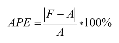
Step 3. Absolute Percentage Errors (APEs) are calculated for each of the synthetic forecasts by age group and any other variables required (e.g., total population; population by five year age groups; percentage of the population aged 65+; dependency ratio; median age; births, deaths, net migration). APE is defined as:

A P E = \frac{| F - A |}{A} * 100 %

where $F$ = forecast and $A$ = actual value.

Step 4. APEs for each variable are arranged by length of forecast horizon in years, and the 80th percentile values are calculated by year up to twenty years out. There are too few error values beyond twenty years. An error tolerance is selected, in this case 5% APE, and the number of whole years into the forecast horizon where the 80th percentile APE remains below the error tolerance is recorded. This is the shelf life of the forecast variable.

Although other error thresholds could have been selected, 5% was chosen in this case because previous focus group research found that 3 to 5% error was regarded as acceptable by forecast users (Wilson and Shalley 2019). Alternative error thresholds could be chosen if desired. The 80th percentile is selected because the number of data values is small and it is best to avoid including very large errors. As an example, Figure 1 below shows the shelf life for the total population of Australia calculated from past errors. The APEs of the thirty synthetic historical forecasts are shown by the gray lines. At ten years out the 80th percentile APE was 4.9%, while at eleven years it was 5.4%. The shelf life is therefore ten years. Note that it is at least 80% likely that forecasts within the shelf life are within 5% error. At the end of the shelf life 80% of forecasts are likely to be within 5% error, while earlier in the shelf life it is greater than 80% (Figure 1), hence the use of the phrase “at least 80% likely” when applied to forecasts later in the article.

Figure 1.

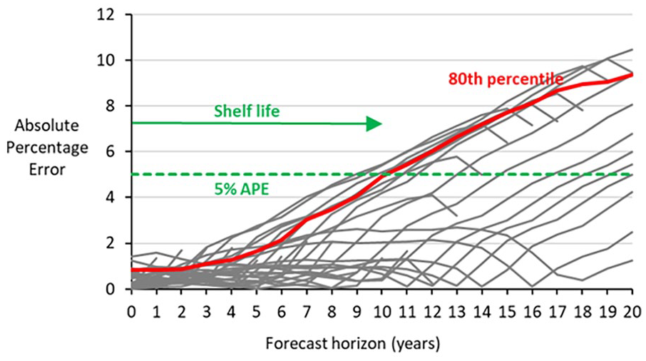
Synthetic historical forecast errors and shelf life for the total population of Australia.

Step 5. For each variable in the current set of population forecasts, a shelf life is applied. For example, if the errors of the synthetic historical forecasts indicate that for age group x the 80th percentile APE is within 5% for up to seven years ahead, then the 2021-based forecast for age group x is allocated a seven year shelf life. Graphs are created in which the shelf life is marked on the current forecasts as a dashed green line. This effectively tells users: “these forecasts are at least 80% likely to be within the chosen error tolerance and should be accurate enough for most purposes.”

Forecasts beyond the shelf life are depicted by a dotted orange line or a red line. The orange line depicts forecasts where the 80th percentile APE has passed 5% error but not 10% (twice the value of the shelf life error threshold). Beyond the 10% cut-off, forecasts are shown by a red line which warns users “be careful: errors could be high.” Similarly, tables or spreadsheets of population data can be shown using green for forecasts within the shelf life and orange and red for those further out.

It should be emphasized that not all forecasts within the shelf life are guaranteed to lie within the selected error tolerance. Because the 80th percentile APE has been selected, some forecasts can be expected to exceed the error tolerance (see Figure 1, for example). In addition, forecasts depicted in orange and red will not necessarily be highly erroneous. The error distribution is relatively wide for these forecasts, especially in the red when the 80th percentile APE has exceeded 10%. These forecasts might be highly erroneous, but they could also turn out to be quite accurate as well.

2.2. Data and Methods for Preparing Forecasts

Both current and synthetic historical population forecasts for Australia were prepared using a cohort-component projection model in which the population was divided by sex and single years of age (Wilson and Rees 2021). There is a small difference with a “standard” cohort-component model in the way international migration is handled. Preliminary international migration is projected using age-specific emigration rates multiplied by populations-at-risk with immigration projected directly as flows; proportional adjustments are then applied to these preliminary migration projections by the projection program to achieve consistency with an assumed total net international migration level (e.g., 200,000 net migration per year). There is a long history in Australia of formulating high-level migration assumptions in terms of annual net international migration totals.

For the current set of forecasts, the jump-off populations consisted of preliminary 2021 Estimated Resident Populations (ERPs) published by the Australian Bureau of Statistics (ABS 2022a). These are based on 2021 Census counts but adjusted for the small proportion of people missed by the census and the small timing difference between census night and the mid-year reference date of ERPs. The long-run Total Fertility Rate (TFR) was set at 1.60, fractionally below TFRs observed in recent years due to expectations of sustained low fertility in Australia (McDonald 2020). Indications of a short-term recovery in fertility after a brief drop during the COVID lockdowns (ABS 2022a) meant that the TFR was set a little above the long-run assumption for the first two years of the forecasts. Net international migration was assumed to be 225,000 per year from 2025- 2026 onwards, close to the pre-COVID annual average of the last decade (ABS 2022a), but slightly above it due to the recent election of a federal government which implemented a short-term increase to the number of places in the Migration Program (O’Neil 2022). Life expectancy at birth was projected using Ediev’s (2008) extrapolative model of mortality, with a small adjustment made over the first two years of the forecast horizon for an expected short-term drop in life expectancy due to COVID deaths (ABS 2022b). After that, long-run trends in mortality are assumed to continue.

The synthetic historical population forecasts were prepared with an assumption-setting approach as close as possible to the current set of forecasts. It excluded the use of any additional forecaster judgment in the assumptions because this is very difficult to replicate for past time periods. The assumption-setting approach taken for all synthetic historical forecasts was as follows. For each historical forecast (1991-based, 1992-based, 1993-based, etc.), the Total Fertility Rate was assumed to remain constant at the average rates of the last three years. For international migration, the average annual net international migration gain of the last ten years was assumed to remain constant into the future. A ten year period was selected due to the considerable volatility of migration in Australia. For mortality, the extrapolative model of Ediev (2008) was applied up to the year before each jump-off year and the resulting projected life expectancies and age-specific deaths rates were used. The jump-off year ERPs were those available one year after the jump-off reference date. These populations differ slightly from the latest time series dataset of ERPs because of adjustments made following subsequent censuses and a one-off adjustment for years 1991 to 2011 made by the ABS after the 2011 Census (ABS 2013).

Jump-off populations and data to calculate forecast assumptions were obtained from the ABS. TFRs and net international migration totals were sourced from the ABS publication National, State and Territory Population (ABS 2022a) and its predecessor Australian Demographic Statistics (ABS 2019). Births and deaths by age and sex were obtained from the ABS Data Explorer tool at https://explore.data.abs.gov.au/, which provides data for recent decades; deaths data prior to the 1970s were obtained from the Australian Demographic Databank (Smith 2009). Immigration and emigration by age and sex were estimated by adjusting initial immigration and emigration numbers to be consistent with cohort population change over the most recent intercensal interval for each set of forecasts. These five-year intervals are bounded by two sets of ERPs based on census counts and broken down by age and sex. Immigration and emigration were proportionally adjusted to match cohort residual net migration, calculated as cohort population change after accounting for deaths. Past ERPs by age and sex were obtained from National, State and Territory Population or Australian Demographic Statistics for 2005 onwards; for years 1991 to 2004 ERPs were published in Population by Age and Sex, Australian States and Territories (ABS 2004).

3. Results

3.1. Estimated Shelf Lives

Shelf lives were calculated for a selection of variables based on the Absolute Percentage Errors (APEs) from the synthetic historical population forecasts. These are illustrated in Figure 2. Using the chosen cohort-component population projection model and assumption-setting approach described above, 80% of past forecasts were within 5% APE for ten years into the forecast horizon for the total population. Therefore, the forecast of Australia’s total population is considered to have a ten year shelf life.

Figure 2.

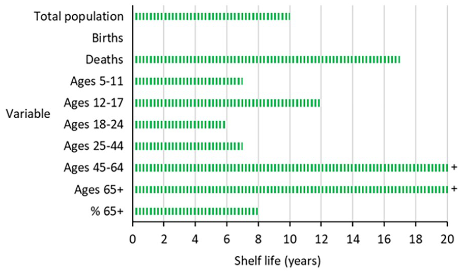
The shelf lives of population forecasts for Australia for selected variables.

For births, there is a shelf life of zero years! Even for the first projection interval the 80th percentile of APE is (just) outside the 5% APE cut-off. This is disappointing, but it underscores the difficulty of forecasting births. It is influenced by errors of age-specific fertility rates and the size of the childbearing-age female population, both of which are hard to forecast. In contrast, mortality usually exhibits relatively stable trends, which is reflected in a seventeen year shelf life for deaths.

For forecasts of primary school children aged 5 to 11 the shelf life is seven years, while for secondary school children aged 12 to 17 it is twelve years. From five years into the forecast horizon, the population of 5 to 11 year olds starts to include birth cohorts which were not born at the jump-off year, so the forecast is affected by the uncertainty of birth forecasts from this time onwards. In fact, the 80th percentile APE line (not shown) is non-linear, the values are quite low until five years out and then rise rapidly over the next few years of the forecast horizon.

The Australian population of 18 to 24 years old, those in education or training, or new labor force entrants, can only be reliably forecast for six years ahead. The forecast for those aged 25 to 44 is similar, with a shelf life of just seven years. These relatively short shelf lives largely reflect the high rates and high volatility of international migration to and from Australia, which is concentrated in the young adult ages. However, the population aged 45 to 64 can be forecast with much greater success, having a shelf life of more than twenty years.

The two variables at the bottom of Figure 1 illustrate the reliability of population aging forecasts. The number of people aged 65+ has a forecast shelf life of more than twenty years. At these ages, migration rates are relatively low and mortality rates become increasingly important with rising age. The dominance of a demographic process (mortality) which can be forecast relatively accurately for quite a few years into the future means that forecasts of the 65+ population are also likely to be quite accurate for many years ahead. However, the percentage of the population aged 65+ has a shorter shelf life of just eight years. This is due to much more uncertainty in the forecast of the population aged 0 to 64 years old in the denominator of the 65+ percentage when it is expressed as

\frac{P_{65 +}}{(P_{0 - 64} + P_{65 +})} * 100 %

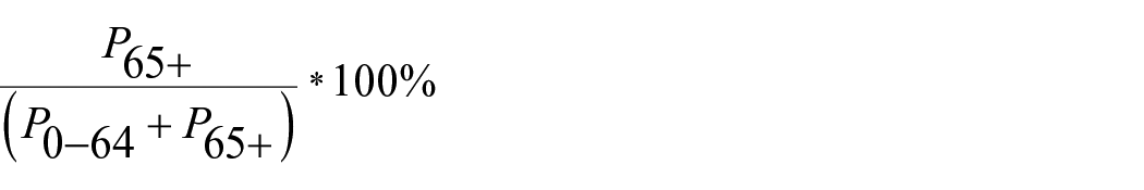
where $P$ = population.

The shelf lives of population forecasts for Australia by five year age group are shown in Figure 3. The shelf lives of forecasts for age groups 55 to 59 years old and above are more than 20 years, reflecting low migration rates and increasing mortality rates with age. The shortest shelf lives are for young children (ages 0–4) and young adults in the peak migration age groups (especially ages 25–29). Interestingly, the age pattern of shelf lives approximates the inverse of the typical migration age pattern. In fact, it largely reflects the relative importance of demographic processes occurring at each age and their degree of uncertainty: at the youngest childhood ages, births and reasonably high rates of migration (both uncertain); at the young adult ages, high rates of migration (uncertain); at the older working ages, migration (uncertain) and mortality (fairly certain) but with both at low rates; and at the oldest ages, mortality. In addition, the shelf lives are influenced to some extent by uncertainty propagating up the ages as cohorts get older over time.

Figure 3.

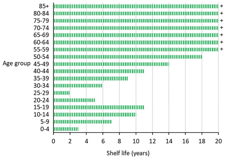
The shelf lives of population forecasts for Australia by five year age group.

3.2. Visualizing the Uncertainty of 2021-Based Forecasts for Australia

A selection of the shelf lives described above, along with traffic lights color-coding, are now shown applied to the current 2021-based population forecasts for Australia. Figure 4 presents observed and forecast total populations of Australia out to 2041. Forecasts within the ten year shelf life are shown by the dashed green line while those beyond it are depicted by the dotted orange line. The 2021 population of 25.7 million is forecast to increase to 29.0 million by the end of the shelf life in 2031. Forecasts within the shelf life are likely to be within 5% error during the shelf life and thus deemed “safe for consumption.” “Likely” in this context means: if error patterns of the future remain the same as those of the past, at least 80% of forecasts will be within 5% error during the shelf life. So it is important to emphasize that errors could still exceed 5% within the shelf life. By 2041 the forecast population is 32.4 million, a figure which could well be in error by more than 5%, though it is unlikely to exceed 10% error.

Figure 4.

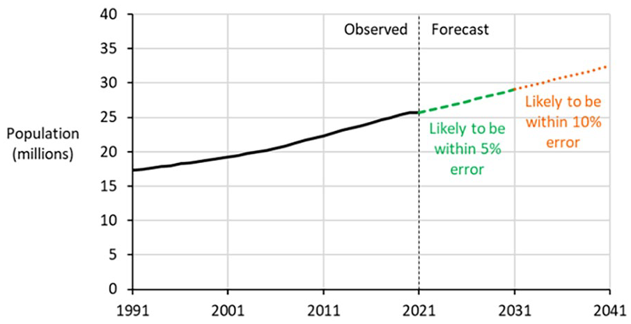
Forecasts of the total population of Australia, 2021 to 2041.

Figure 5 presents forecasts of the population aged 65 and above, with the top graph showing the numbers aged 65+ and the bottom graph the percentage of the population in this age group. The population aged 65+ is forecast to increase from 4.3 million in 2021 to 6.7 million by 2041. Given that the shelf life exceeds twenty years, this forecast is likely to be within 5% error for the whole 2021 to 2041 forecast horizon. The percentage of the population aged 65+ is forecast to increase from 16.8% in 2021 to 19.0% by the end of the shelf life in 2029. By 2041, the percentage is forecast to have risen to 20.6%, but this figure is subject to greater uncertainty (though it is likely to be within 10% error).

Figure 5.

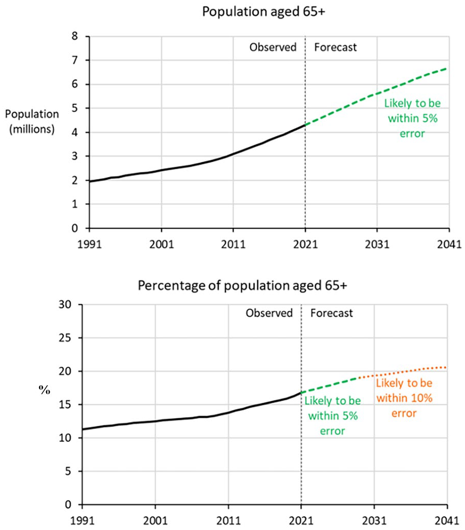
Forecasts of the population of Australia aged 65+, 2021 to 2041.

Forecasts of births and deaths are shown in Figure 6. For births, the magnitude of errors from the synthetic historical forecasts is such that the 80th percentile APE exceeds 5% from the very start of the forecast horizon. The shelf life is zero years and forecasts of the annual number of births should be used with caution. Births are likely to be within 10% error for the first three years, but then could be subject to higher errors after that (shown by the thick red line). The seventeen year shelf life for deaths suggests that the forecast annual number of deaths should be fairly accurate out to the 2037-2038 projection interval, the end of the shelf life. However, it is possible that COVID may interfere with the assumed constancy of error patterns. In the current set of forecasts, a short-term increase in deaths is forecast for the immediate term because of the considerable number of deaths currently occurring due to COVID (ABS 2022b). It is based on the assumption that “normal” trends in mortality will resume after two years into the forecast horizon, an assumption which has had to be made using judgment rather than strong evidence.

Figure 6.

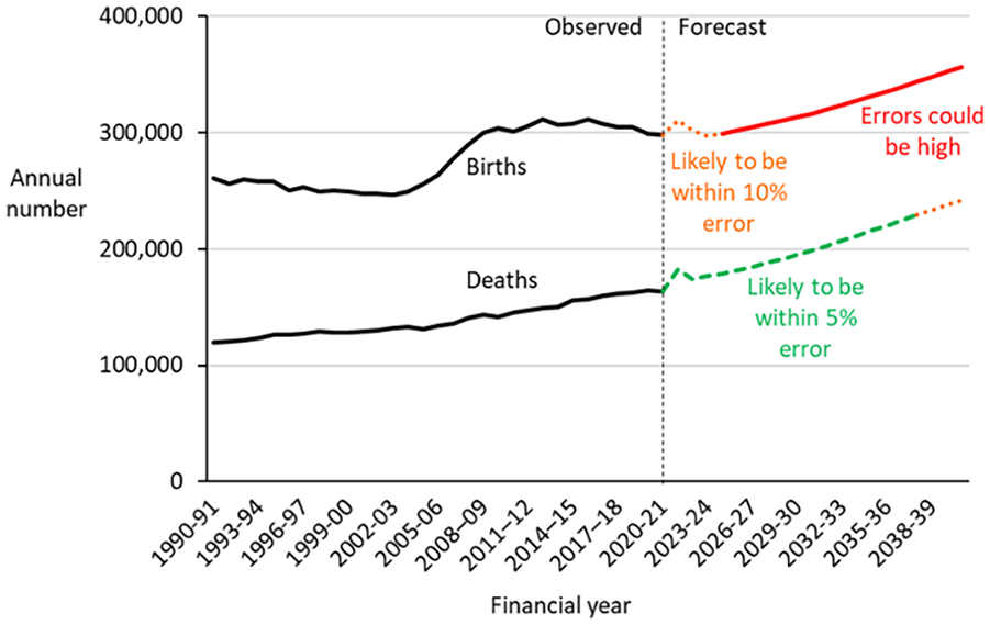
Forecasts of births and deaths in Australia, 2021 to 2041.

Forecasts in tabular or spreadsheet form can be presented using the same general approach but with background shading to indicate whether forecasts are within the shelf life or not. As an example, Figure 7 shows a small section of a spreadsheet with selected variables from the 2021-based Australian population forecasts. The green cells indicate forecasts within the shelf life, whilst the orange cells indicate forecasts likely to be within 10% error. Red colored cells warn users that forecasts could well exceed 10% error. Cells containing population variables without shading (in column B) indicate observed data.

Figure 7.

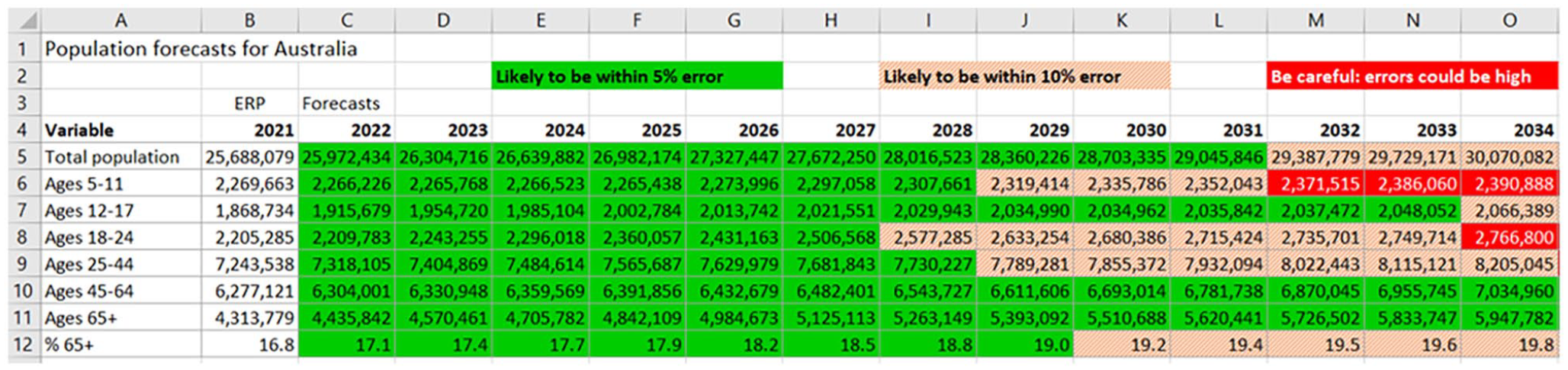
Population forecasts for Australia for selected variables.

4. Discussion and Conclusions

4.1. Value and Uses of the Approach

The main contribution of this article is an approach to estimating population forecast shelf lives based on synthetic historical forecast errors, and the application and illustration of shelf lives for current forecasts. The approach is relatively simple and makes use of existing deterministic models and their data inputs. The easily understood concept of the shelf life of perishable foods transfers easily to forecasts, referring to the period of time into the future during which a population forecast is likely to be “safe to consume.” The historical forecast error/shelf life approach provides a simple means of communicating forecast uncertainty where probabilistic methods cannot be implemented. The visualization of population forecast shelf lives provides users with basic information about forecast uncertainty. Graphs can be simple and easily interpretable. Users can clearly see how far into the future forecasts are at least 80% likely to remain within 5% error (or a different error tolerance if necessary) and when they are not. Color coding and formatting of forecasts within the shelf life (green) and beyond (orange and red) can be applied both graphically and in tables and spreadsheets. Some users might wish to interpret population numbers within the shelf life as forecasts, and label those appearing further into the future as projections.

Shelf lives are not only useful for indicating how far into the future a population is likely to be accurately forecast. They also underscore how forecast uncertainty differs between variables. Comparisons of the shelf lives of births and deaths, and the number of people aged 65+ and the percentage of the population aged 65+, emphasize how some variables can be forecast far out into the future with reasonable accuracy whilst others cannot. It is also important to stress that even in circumstances when the total population shelf life does not extend far into the future, it does not mean that the entire forecast should be discarded beyond that. It could well be that the shelf life of the key population variable of interest (e.g., the population aged 75+) might extend far enough into the future to be of use.

There are several avenues for further exploration and application. The approach may highlight where data and projection methods need improvement. Very short shelf lives, such as that for births in the case study presented earlier, could indicate problems with input data and / or forecasting methods. It is certainly the case that fertility rates are challenging to forecast, even in the short term. The fact that preliminary births data in Australia is based on the number of birth registrations over a defined period (ABS 2022a), rather than the number of births which actually occurred, may also be a contributing factor. Registration delays and catch-ups can affect the apparent trend in fertility.

Comparisons between two different models for projecting the same population could be made by creating synthetic historical forecasts and comparing errors and shelf lives. If a new forecasting method is proposed, such as for fertility, then it could be evaluated against the current method using this approach. The focus of the comparison becomes: does the new method lower forecast errors and extend shelf lives?

The historical forecast error/shelf life approach could be applied to other countries and expanded to sub-national geographies. It would be useful for the many users of state and territory population forecasts to have information on the shelf lives of those forecasts. It would also be interesting to see how shelf lives vary between jurisdictions and forecast variables. In applications to other countries, forecasts for populations generally experiencing more volatile migration trends would probably have shorter shelf lives. Countries which have experienced large changes in life expectancy trends over recent decades would probably have shorter shelf lives of deaths and populations at the oldest age groups than shown in the case study of Australia.

Finally, the approach could also be used in conjunction with, rather than as an alternative to, probabilistic population forecasts. Shelf lives could be applied to probabilistic forecasts and marked out on graphs and tables of prediction intervals. The shelf life could be defined as the period into the future where the 80 percent prediction interval of the probabilistic forecast remains within a specified percentage of the median forecast. These shelf lives could also act as a plausibility check on probabilistic forecasts generated by statistical models and/or expert judgment. If the differences with the length and pattern of shelf lives based on synthetic historical forecast errors were considerable, then modelers would need to decide whether the differences were acceptable or plausible.

4.2. Strengths and Limitations

There are, of course, some limitations of the suggested approach. The assumption of past error patterns remaining unchanged into the future will probably be violated to some extent. Demographic trends may become more, or perhaps less, volatile in the future. Changes to migration policy can hugely influence population growth and development. Major events such as the COVID pandemic, economic depression, and war can massively disrupt demographic trends. Should past forecast errors be adjusted or calibrated in some manner to allow for this? Possibly, but it would be challenging to make those adjustments, and it might come at the cost of lower user understanding and confidence in how the uncertainty measures were calculated. In addition, even if error patterns do remain constant into the future, some errors will still exceed the specified error tolerance due to the use of an 80th percentile APE cut-off. Shelf lives are therefore best regarded as guidance about uncertainty rather than anything definitive.

Furthermore, shelf lives are calculated from the errors of a relatively small sample of synthetic “historical” forecasts which may differ from the error pattern had it been possible to create a much larger sample of errors. And these historical forecasts, while not difficult to create, will require a non-trivial amount of an analyst’s time to complete. Furthermore, the graphs (and tables) of population forecasts displaying shelf lives only convey limited information about uncertainty to users. There is no indication of the magnitude of uncertainty as there is with “fan diagrams” (or tables) of probabilistic forecasts which present forecast values at the upper and lower bounds of selected prediction intervals. It should also be noted that historical error values, and therefore shelf life estimates, are specific to a particular projection model, assumption-setting approach, and population. Shelf life estimates are not transferable to other populations or projection methods.

Despite these limitations, I believe the approach has many strengths and potential for application. As noted above, the graphs are fairly simple and easy to comprehend. For many users, a basic distinction between that part of a forecast which is likely to be “reasonably accurate” and that which is not will be sufficient. The way in which forecasts are presented is similar to current approaches. This should make the introduction of forecasts depicting shelf lives relatively straightforward and not require users to undergo a substantial shift in their thinking about forecasts. In addition, forecast uncertainty illustrated through shelf lives is based directly on past error patterns and not from prediction intervals generated via complex statistical models and / or expert judgment. Some users may view the latter as a statistical black box and find the idea of shelf lives calculated from past errors more digestible. Importantly, the use of the current model and assumption-setting approach in creating historical errors ensures that error patterns are relevant to the current set of forecasts.

For population forecasters, the preparation of forecasts with shelf lives does not require any complex statistical modeling of uncertainty. It only requires the deterministic projection model and assumption-setting approach commonly employed by many practitioners and researchers today. It just needs demographic data for the population of interest extending back sufficiently in time to create a set of synthetic historical forecasts. The staff time, input data, and technical expertise required are not nearly as high as that needed if switching to probabilistic forecasts, thereby keeping costs manageable.

The approach can also be easily applied to sub-national geographies so long as there is a sufficiently long time series of past data on current regional boundaries to create the historical forecasts. In Australia, this would include the States and Territories (though it would be more challenging for some sub-state geographies). Given the limited development of probabilistic forecasting methods for sub-national populations, the historical errors / shelf life approach offers a relatively easy way of estimating and communicating forecast uncertainty for these populations.

4.3. Concluding Remarks

The purpose of this article was to set out a relatively simple approach to estimating and communicating population forecast uncertainty to a broad range of users. One key message is that presenting uncertainty graphically using shelf lives and color coding offers a simple way of communicating uncertainty to a broad range of users. A second key point is that, for any population, forecast uncertainty varies according to the demographic variable of interest. It is not possible to simply describe a population forecast as being reliable (however defined) for x number of years into the future. Some forecast variables, such as the population aged 65+, might be reliably forecast long into the future, while others, such as the number of 0 to 4 years old, probably will not.

Ideally, all population forecasts would be accompanied by easily understood information about their uncertainty. This should be seen as “completing the forecast” (Committee on Estimating and Communicating Uncertainty in Weather and Climate Forecasts 2006). If forecasts and their uncertainty are not communicated effectively, then they are much diminished in value. Effective communication of uncertainty in forecasts helps users make better decisions and become more trustful of forecasts (Raftery 2016). I hope the approach described in this article will prove useful for practitioners and users of population forecasts in understanding forecast uncertainty and incorporating it into decision-making.

Footnotes

Acknowledgements

The author thanks the editors and anonymous reviewers for the helpful comments and suggestions which improved the article significantly.

Funding

The author disclosed receipt of the following financial support for the research, authorship, and / or publication of this article: This work was supported by the Australian Research Council Centre of Excellence in Population Ageing Research (project number CE1101029).

Received: January 2023

Accepted: September 2023

References

Alders

Keilman

Cruijsen

2007. “Assumptions for Long-Term Stochastic Population Forecasts in 18 European Countries.” European Journal of Population 23: 33–69. DOI: https://doi.org/10.1007/s10680-006-9104-4.

Alho

J, M.

1990. “Stochastic Methods in Population Forecasting.” International Journal of Forecasting 6 (4): 521–30. DOI: https://doi.org/10.1016/0169-2070(90)90030-F.

Asoze

J. J.

Ševčíková

Raftery

A. E.

2016. “Probabilistic Population Projections with Migration Uncertainty.”

Proceedings of the National Academy of Sciences

113 (23): 6460–5. DOI: https://doi.org/10.1073/pnas.1606119113.

ABS (Australian Bureau of Statistics). 2004. Population by Age and Sex, Australian States and Territories. Available at: https://www.abs.gov.au/AUSSTATS/abs@.nsf/allprimarymainfeatures/58E1FA8F39B39547CA2570D8001B84CC? (accessed December 2022).

ABS (Australian Bureau of Statistics). 2013. Australian Demographic Statistics. Available at: https://www.abs.gov.au/AUSSTATS/abs@.nsf/Lookup/3101.0Main+Features1Dec%202012?OpenDocument (accessed December 2022).

ABS (Australian Bureau of Statistics). 2019. Australian Demographic Statistics. Available at: https://www.abs.gov.au/AUSSTATS/abs@.nsf/Lookup/3101.0Main+Features1Jun%202019 (accessed December 2022).

ABS (Australian Bureau of Statistics). 2022a. National, State and Territory Population. Available at: https://www.abs.gov.au/statistics/people/population/national-state-and-territory-population/mar-2022 (accessed December 2022).

ABS (Australian Bureau of Statistics). 2022b. Provisional Mortality Statistics. Available at: https://www.abs.gov.au/statistics/health/causes-death/provisional-mortality-statistics/latest-release (accessed December 2022).

Bijak

Disney

Findlay

A. M.

Forster

J. J.

Smith

P. W. F.

Wiśniowski

2019. “Assessing Time Series Models for Forecasting International Migration: Lessons from the United Kingdom.” Journal of Forecasting 38: 470–87. DOI: https://doi.org/10.1002/for.2576.

10.

Billari

F. C.

Graziani

Melilli

2012. “Stochastic Population Forecasts Based on Conditional Expert Opinions.” Journal of the Royal Statistical Society: Series A (Statistics in Society) 175 (2): 491–511. DOI: https://doi.org/10.1111/j.1467-985X.2011.01015.x.

11.

Billari

F. C.

Graziani

Melilli

2014. “Stochastic Population Forecasting Based on Combinations of Expert Evaluations Within the Bayesian Paradigm.” Demography 51 (5): 1933–54. DOI: https://doi.org/10.1007/s13524-014-0318-5.

12.

Bohk-Ewald

Myrskylä

2018. “Forecast Accuracy Hardly Improves with Method Complexity When Completing Cohort Fertility.” Proceedings of the National Academy of Sciences 115 (37): 9187–92. DOI: https://doi.org/10.1073/pnas.1722364115.

13.

Bongaarts

Bulatao

R. A.

, eds. 2000. Beyond Six Billion: Forecasting the World’s Population. Washington, D.C.: The National Academies Press. DOI: https://doi.org/10.17226/9828.

14.

Committee on Estimating and Communicating Uncertainty in Weather and Climate Forecasts. 2006. “Completing the Forecast: Characterizing and Communicating Uncertainty for Better Decisions Using Weather and Climate Forecasts.” Washington D.C., USA: The National Academies Press. DOI: https://doi.org/10.17226/11699.

15.

De Valk

H. A. G.

Acostamadiedo

Guan

Melde

Mooyaart

Sohst

R. R.

Tjaden

2022. “How to Predict Future Migration: Different Methods Explained and Compared.” In Introduction to Migration Studies, edited by Scholten

, 463–82, Cham: Springer. DOI: https://doi.org/10.1007/978-3-030-92377-8_28.

16.

Dion

2017. “An Alternative to Fixed Transition Probabilities for the Projection of Interprovincial Migration in Canada.” Population Research and Policy Review 36: 871–901. DOI: https://doi.org/10.1007/s11113-017-9440-6.

17.

Ediev

D. M.

2008. “Extrapolative Projections of Mortality: Towards a More Consistent Method. Part I: The Central Scenario.” Vienna Institute for Demography Working Paper 3/2008. Available at: https://www.oeaw.ac.at/fileadmin/subsites/Institute/VID/PDF/Publications/Working_Papers/WP2008_03.pdf.

18.

Ediev

D. M.

2020. “Mortality Projection.” In Encyclopedia of Gerontology and Population Aging, edited by Gu

Dupre

M. E.

: 1–9. Cham: Springer. DOI: https://doi.org/10.1007/978-3-319-69892-2_557-1.

19.

Fuchs

Söhnlein

Vanella

2021. “Migration Forecasting—Significance and Approaches.” Encyclopedia 1 (3): 689–709. DOI: https://doi.org/10.3390/encyclopedia1030054.

20.

Gleditsch

R. F.

Rogne

A. F.

Syse

Thomas

2021. The Accuracy of Statistics Norway’s National Population Projections. Discussion Papers No. 948, Statistics Norway, Oslo. Available at: https://www.ssb.no/en/forskning/discussion-papers/the-accuracy-of-statistics-norways-national-population-projections.

21.

Graziani

2020. “Stochastic Population Forecasting: A Bayesian Approach Based on Evaluation by Experts.” In Developments in Demographic Forecasting, edited by Mazzuco

Keilman

, 21–42. Cham: Springer. DOI: https://doi.org/10.1007/978-3-030-42472-5_2.

22.

Istat. 2022. Households and Population Projections–Base 1/1/2021. Available at: https://www.istat.it/en/archivio/274900 (accessed December 2022).

23.

Janssen

2018. “Advances in Mortality Forecasting: Introduction.” Genus 74 (21). DOI: https://doi.org/10.1186/s41118-018-0045-7.

24.

Keilman

2001. “Data Quality and Accuracy of United Nations Population Projections, 1950–95.” Population Studies 55 (2): 149–64. DOI: https://doi.org/10.1080/00324720127686.

25.

Keilman

2008. “European Demographic Forecasts Have Not Become More Accurate Over the Past 25 Years.” Population and Development Review 34 (1): 137–53. DOI: https://doi.org/10.1111/j.1728-4457.2008.00209.x.

26.

Keilman

2019. “Erroneous Population Forecasts.” In Old and New Perspectives on Mortality Forecasting, edited by Bengtsson

Keilman

, 95–111. Cham: Springer. DOI: https://doi.org/10.1007/978-3-030-05075-7_9.

27.

Keilman

2020. “Uncertainty in Population Forecasts for the Twenty-First Century.” Annual Review of Resource Economics 12 (1): 449–70. DOI: https://doi.org/10.1146/annurev-resource-110319-114841.

28.

Keilman

Pham

D. Q.

Hetland

2002. “Why Population Forecasts Should be Probabilistic—Illustrated by the Case of Norway.” Demographic Research 6 (15): 409–54. DOI: https://doi.org/10.4054/DemRes.2002.6.15.

29.

Keyfitz

1981

“The Limits of Population Forecasting.”

Population and Development Review 7 (4): 579–93. DOI: https://doi.org/10.2307/1972799.

30.

McDonald

2020. “A Projection of Australia’s Future Fertility Rates.” Centre for Population Research Paper, Australian Government, Canberra, ACT, Australia. Available at: https://population.gov.au/research/research-fertility.

31.

New Zealand Ministry for Primary Industries. 2016. How to Determine the Shelf Life of Food. Wellington: Ministry for Primary Industries. Available at: https://www.mpi.govt.nz/dmsdocument/12540-how-to-determine-the-shelf-life-of-food-guidance-document.

32.

Office for National Statistics (ONS). 2015. National Population Projections Accuracy Report. London, UK: Office for National Statistics. Available at: https://www.ons.gov.uk/peoplepopulationandcommunity/populationandmigration/populationprojections/methodologies/nationalpopulationprojectionsaccuracyreport.

33.

O’Neil

2022. “Australia’s Migration Future.” Available at: https://minister.homeaffairs.gov.au/ClareONeil/Pages/australias-migration-future.aspx (accessed December 2022).

34.

Raftery

A. E.

2016. “Use and Communication of Probabilistic Forecasts.” Statistical Analysis and Data Mining 9: 397–410. DOI: https://doi.org/10.1002/sam.11302.

35.

Raftery

A. E.

Ševčíková

Heilig

G. K.

2012. “Bayesian Probabilistic Population Projections for All Countries.”

Proceedings of the National Academy of Sciences

109 (35): 13915–21. DOI: https://doi.org/10.1073/pnas.1211452109.

36.

Raftery

A. E

Ševčíková

2021. “Probabilistic Population Forecasting: Short to Very Long-Term.” International Journal of Forecasting 39 (1): 73–97. DOI: https://doi.org/10.1016/j.ijforecast.2021.09.001.

37.

Rayer

Smith

S. K.

Tayman

2009. “Empirical Prediction Intervals for County Population Forecasts.” Population Research and Policy Review 28 (6): 773–93. DOI: https://doi.org/10.1007/s11113-009-9128-7.

38.

Rees

Kupiszewski

Eyre

Wilson

Durham

2001. The Evaluation of Regional Population Projections for the European Union. Eurostat Working Paper 3/2001/E/no. 9. Available at: https://ec.europa.eu/eurostat/web/products-statistical-working-papers/-/ks-ap-01-041.

39.

Smith

2009. “The Australian Demographic Data Bank, 1901–2003.” Canberra, ACT, Australia: Australian Social Science Data Archive, The Australian National University.

40.

Smith

S. K.

Sincich

1988. “Stability Over Time in the Distribution of Population Forecast Errors.” Demography 25 (3): 461–74. DOI: https://doi.org/10.2307/2061544.

41.

Smith

S. K.

Tayman

2003. “An Evaluation of Population Projections by Age.” Demography 40 (4): 741–57. DOI: https://doi.org/10.1353/dem.2003.0041.

42.

Smith

S. K.

Tayman

Swanson

D. A.

2013. A Practitioner’s Guide to State and Local Population Projections. Dordrecht: Springer.

43.

Spiegelhalter

Pearson

Short

2011. “Visualizing Uncertainty About the Future.” Science 333: 1393–400. DOI: https://doi.org/10.1126/science.1191181.

44.

Statistics Netherlands. 2021. Forecast: Population Growth Picks Up Again. Available at: https://www.cbs.nl/en-gb/news/2021/50/forecast-population-growth-picks-up-again (accessed December 2022).

45.

Statistics New Zealand. 2016. How Accurate Are Population Estimates and Projections? An Evaluation of Statistics New Zealand Population Estimates and Projections, 1996–2013. Available at: https://www.stats.govt.nz/methods/how-accurate-are-population-estimates-and-projections (accessed December 2022).

46.

Statistics New Zealand. 2022. National Population Projections: 2022(base)–2073. Available at: https://www.stats.govt.nz/information-releases/national-population-projections-2022base2073/ (accessed December 2022).

47.

Stoto

M. A.

1983. “The Accuracy of Population Projections.” Journal of the American Statistical Association 78 (381): 13–20. DOI: https://doi.org/10.2307/2287094.

48.

Tayman

2011. “Assessing Uncertainty in Small Area Forecasts: State of the Practice and Implementation Strategy.” Population Research and Policy Review 30 (5): 781–800. DOI: https://doi.org/10.1007/s11113-011-9210-9.

49.

United Nations Population Division. 2022. “World Population Prospects 2022.” Available at: https://population.un.org/wpp/

50.

Vandresse

2016. Projection of Internal Migration Based on Migration Intensity and Preferential Flows. Working Paper 10-16, Federal Planning Bureau, Belgium. Available at:https://www.plan.be/publications/publication-1630-en-projection_of_internal_migration_based_on_migration_intensity_preferential_flows.

51.

Van Duin

2017. Quasi Stochastic Population Forecasts. Discussion Paper 2017-01, Statistics Netherlands, The Hague. Available at: https://www.cbs.nl/en-gb/background/2017/04/quasi-stochastic-population-forecasts.

52.

Wilson

2007. “The Forecast Accuracy of Australian Bureau of Statistics National Population Projections.” Journal of Population Research 24 (1): 1–27. DOI: https://doi.org/10.1007/BF03031880.

53.

Wilson

2012. “Forecast accuracy and uncertainty of Australian Bureau of Statistics state and territory population projections.” International Journal of Population Research. DOI: http://doi.org/10.1155/2012/419824.

54.

Wilson

2018. “Communicating Population Forecast Uncertainty Using Perishable Food Terminology.” Research Brief RB03/2018, Northern Institute, Charles Darwin University. Available at: https://researchers.cdu.edu.au/en/publications/communicating-population-forecast-uncertainty-using-perishable-fo.

55.

Wilson

Brokensha

Rowe

Simpson

2018. “Insights From the Evaluation of Past Local Area Population Forecasts.” Population Research and Policy Review 37 (1): 137–55. DOI: https://doi.org/10.1007/s11113-017-9450-4.

56.

Wilson

Rees

2021. “A Brief Guide to Producing a National Population Projection.” Australian Population Studies 5 (1): 77–101. DOI: https://doi.org/10.37970/aps.v5i1.84.

57.

Wilson

Shalley

2019. “Subnational Population Forecasts: Do Users Want to Know About Uncertainty?” Demographic Research 41 (13): 367–92. DOI: https://doi.org/10.4054/DemRes.2019.41.13.

Visualizing the Shelf Life of Population Forecasts: A Simple Approach to Communicating Forecast Uncertainty

Abstract

Keywords

1. Introduction

2. Data and methods

2.1. Shelf Life Estimation

2.2. Data and Methods for Preparing Forecasts

3. Results

3.1. Estimated Shelf Lives

3.2. Visualizing the Uncertainty of 2021-Based Forecasts for Australia

4. Discussion and Conclusions

4.1. Value and Uses of the Approach

4.2. Strengths and Limitations

4.3. Concluding Remarks

Footnotes

Acknowledgements

Funding

References