
Abstract
The labor force surveys (LFS) of all EU countries underwent a substantial redesign in January 2021. To ensure coherent labor market time series for the main indicators in the Norwegian LFS, we model the impact of the redesign. We use a state-space model that takes explicit account of the rotating pattern of the LFS. We also include auxiliary variables related to employment and unemployment that are highly correlated with the LFS variables we consider. The results of a parallel run are also included in the model. The purpose of the article is to quantify the structural breaks due to the redesign. This article makes two contributions to the literature on the effects of redesign in surveys with a rotating panel, such as the LFS. First, we suggest a symmetric specification of the process of the wave-specific effects. Second, we account for substantial fluctuations in the labor force estimates due to the COVID-19 pandemic in the time around the LFS redesign by applying time-varying hyperparameters for both the LFS variables and the auxiliary variables. The specification with time-varying hyperparameters shows a better fit compared to the specification with time-invariant hyperparameters.
1. Introduction
Time series from LFS that describe the situation in the labor market are valuable for many users. These series provide important information for fiscal and monetary policy and wage bargaining in Norway, either directly or indirectly through the National Accounts. Therefore, they must be comparable over time, as it is otherwise difficult to interpret them. From time to time, it is necessary to redesign the surveys, for instance, in connection with international regulations. Such changes require correcting time series to make them comparable over time. The purpose of this article is to quantify the structural breaks in the Norwegian LFS due to a redesign.
From the beginning of 2021, the LFS in 34 European countries underwent a substantial redesign in accordance with the new regulation for integrated European social statistics (IESS). The redesign took place in all member states of the European Union, the three EFTA countries (Iceland, Norway, and Switzerland), as well as in four candidate countries (Montenegro, North Macedonia, Serbia, and Turkey). The purpose of the redesign was to standardize definitions and thereby increase comparability between countries. The redesign implied a modified questionnaire, where question sequences, formulations, and answer alternatives have changed. In addition to the changes that followed from IESS regulation, further changes were made in the Norwegian LFS. The sampling unit was changed from family to person, and indirect interviewing was ended.
How to best quantify and implement corrections related to redesign depends on the information at hand: for instance, whether one has parallel surveys or auxiliary variables at one’s disposal. One approach is to have parallel data collection where the data under the old and new survey designs are collected side by side for some period. Ideally, this should be arranged as a randomized experiment. With adequate sample sizes, estimates of structural breaks can be made by contrasting design-based sample estimates under the different designs. These estimates can be made right after the period of data collection, to get timely break estimates. This is an approach with low risk, but expensive, and requires that the survey organization manages to have two sizable surveys running at the same time.
Time series models can also be applied in connection with repeated surveys. Repeated surveys may be either non-overlapping or overlapping. In the former case, the same observational unit is only observed once and in the latter case, it is observed more than once. If one has overlapping data at hand, one may account for the autocorrelation in survey errors stemming from the fact that an observational unit occurs more than once. The main reason for using time series models is related to small sample sizes, that is, one is not willing to trust the pure estimates based on the surveys alone but prefers to draw on extra information. Such additional information is provided by the history of the target series, data from other domains and information from auxiliary variables that are correlated with the variables of concern.
For general articles about time series modeling of repeated surveys reference is made to Scott and Smith (1974) and Scott et al. (1977) (see also the survey by Pfeffermann 2022). These authors were the first to suggest using time series models not only for survey errors, but also for population values. Pfeffermann (1991) and Pfeffermann et al. (1998) made an important extension by decomposing the population value into trend, seasonal, and irregular components alongside modeling the autocorrelation in survey errors due to a design based on rotating panel data. A common approach is to use structural time series models utilizing the state-space form, see for instance Harvey (1989).
We have a narrower aim in this article since we do not intend to use time series models to estimate population values but only to obtain estimates of the structural break brought about by the redesign of the LFS. To this end, it is important to have a model that captures different properties of the time series and which also incorporates information from auxiliary time series and parallel runs for the LFS data. Intervention effects which are aimed at capturing the effect of redesigns are added to the structural time series model.
The Norwegian LFS follow a rotating design, whereby each respondent participates (in the absence of nonresponse) eight times over a two-year period, making it possible to divide the sample into eight waves. The modeling strategy follows a disaggregated approach in that the modeling is conducted for different domains. We consider four domains by distinguishing between young men and women (15–24 years), and “older” persons (25–74 years) of both sexes. The aggregated estimates are derived from this disaggregated information.
Our analysis is carried out within a structural time series framework using state-space models on monthly wave-divided data from January 2006 to October 2021. The article looks at persons aged 15 to 74, since they are the age group for which we have data both before and after the LFS redesign. We follow the tradition introduced by Pfeffermann (1991) and further developed by, for example, Van den Brakel and Krieg (2009, 2015). We model time series for both employed and unemployed persons. The modeled time series are characterized by different latent components. The time series for the eight waves are assumed to share a common trend component, a common seasonal component, and a common irregular component. Beyond the common components, two other components are added, that is, wave-specific effects and survey errors. Finally, a structural break component is included to capture the possible break due to the 2021 redesign of the LFS.
Besides the wave information, we utilize auxiliary information from registers. For the LFS estimates of for employment, we use registered employees as auxiliary information; and for the LFS estimates of for unemployment, we derive comparable unemployment estimates from the register. The auxiliary variable is assumed to have its own trend, seasonal, and irregular component. This auxiliary information is essential for identifying the effects of the redesign of the LFS since the redesign does not influence the register data and since the time series from the LFS and the register are closely interlinked. We use an auxiliary variable in conjunction with each estimation. Thus, for each domain, we consider modeling a vector with nine elements, where eight are from the LFS, and one is from the register.
The importance of having access to auxiliary variables has long been recognized for example, Tiller (1992) suggested improving the population estimates by applying auxiliary variables. The use of auxiliary variables was developed further by Harvey and Chung (2000), and the approach is used in, for example, Van den Brakel and Michiels (2021). Harvey and Chung (2000) find a common trend between LFS figures and claimant counts in the United Kingdom. Furthermore, results in Van den Brakel and Krieg (2015, 2016) indicate a common trend for the LFS and a register variable for the Netherlands. Schiavoni et al. (2021) apply a common trend for Google trends search variables in a model with LFS.
In our context, the role of auxiliary variables is deemed very important since they are correlated with the LFS variables but not impacted by the redesign of the LFS. We allow the two trend components, related respectively to the LFS and the register data, to be interlinked. This assumption concerning the trend is essential because this is the only channel through which we allow the auxiliary variables to influence the estimated hyperparameters and extracted components that one ends up with for the LFS time series. The correlation needs to be sizeable, and the later empirical analysis shows that the two trend components are closely tied together for all the considered domains for both employment and unemployment. Therefore, the LFS population estimates and the register estimates approximately share a common trend.
It is important to account for wave-specific effects (also referred to in the literature as rotating group bias), as shown already by Stephan et al. (1954), Hansen et al. (1955), and Bailar (1975). Krueger et al. (2017) show that these biases can evolve much over time. Therefore, it seems suitable to let the wave-specific components be time-varying as in Van den Brakel and Krieg (2009). This allows the rotation group bias to change from one period to the next in an unsystematic way. It is customary to treat the different waves in an asymmetric way, either by assuming that one of them is not encumbered by systemic bias or by assuming that all of them are biased and treating one of them as a residual wave.
A novel contribution of our analysis is the treatment of the wave-specific effects. In contrast to Statistics Netherlands, which measures the wave-specific effects relative to the first wave (see Van den Brakel and Krieg 2009, 2015), we follow Elliott and Zong (2019) and impose that the wave-specific effects sum to zero. However, in contrast to Elliott and Zong (2019), we do this in a symmetric way in which we do not treat one wave as residual, thereby placing less weight on it. The way one models the wave-specific component may have consequences for the estimates of the structural break and potentially to a larger degree for the smoothed estimates of other latent components.
An important question is how to model the effects of the redesign. Van den Brakel et al. (2008) and Van den Brakel and Roels (2010) apply intervention analysis for estimating structural break within the framework of structural time series models. van den Brakel and Krieg (2015) include auxiliary variables when estimating the structural break. They also incorporate information from a parallel survey to get a prior estimate of the structural break. Bollineni-Balabay et al. (2016) consider survey redesigns that lead to a structural break in both the level and variance. We account for the structural break in the levels but assume, implicitly, that the redesign does not impact variances. In our state-space model, we apply information from a small parallel survey carried out in the last quarter of 2020. This parallel survey helps us quantify the structural break for the first wave (i.e., for those participating in the survey for the first time), see also Van den Brakel and Krieg (2015).
The presence of COVID-19 induced us to allow for time-varying hyperparameters. It led to large fluctuations in the labor market. During the corona pandemic, unemployment in many countries increased sharply within a short period of time. This feature makes it problematic to assume that the population variables follow a time-invariant process. Van den Brakel et al. (2022) suggest allowing a more flexible trend in such periods and using it in preparing population estimates during the corona period for the Netherlands. Gonçalves et al. (2022) use the same type of flexible trend to produce population estimates for Brazil. A similar approach was also applied by Bollineni-Balabay et al. (2016), who considered breaks in both level and variance due to survey redesigns. When estimating the structural break due to the redesign, we pursue the same approach to accommodate the large fluctuations in the labor market. In contrast to both Bollineni-Balabay et al. (2016) and Van den Brakel et al. (2022), we include an auxiliary variable. We use time-varying hyperparameters for both the LFS variables and the auxiliary variable in a model for quantifying the structural break due to survey redesign. These time-varying hyperparameters are specified such that they allow for a more flexible trend through the COVID-19 pandemic. We consider this model augmentation as the second contribution of our article.
The remainder of this article is organized in the following way: Section 2 describes the redesign of the Norwegian LFS and presents the data used in the analysis. It describes how the monthly wave series are constructed. The section also presents the redesign of the survey in 2021 and provides information about the register data used. Finally, we describe a parallel survey carried out in the last quarter of 2020. Section 3 presents the time-series model we use to estimate the structural break due to the redesign. We comment on issues related to the state-space model used for estimation. This section also covers how we handle the redesign of the survey and how we take account of the extensive labor market fluctuations during the COVID-19 pandemic. In Section 4, we report our empirical results. Here, we also compare our empirical results with those from a model specification that does not account for higher fluctuations in the labor market during the COVID-19 pandemic. Section 5 provides some conclusions. In the Appendix (Section 6), we present our estimation of the autocorrelation parameters of the survey errors and provide a detailed specification of our state-space model. Section Supplemental Documentation contains additional information.
2. About the Data
Statistics Norway has carried out LFS since 1972. Over the years, the survey has been subject to several changes. In this article, we will use data from January 2006 (2006M1). Therefore, the description here applies to the LFS from 2006. The last observation available when the structural breaks were estimated was from 2021M10.
Subsection 2.1 presents the Norwegian LFS from 2006 (and until 2020), while Subsection 2.2 presents the changes in the LFS from 2021. The auxiliary variables are presented in Subsection 2.3, while Subsection 2.4 discusses parallel data collection in the LFS in 2020Q4. Tables 1 and 2 show descriptive statistics for both the LFS variables and the register variables as well as correlations between them, and these tables will be referred to throughout the section.
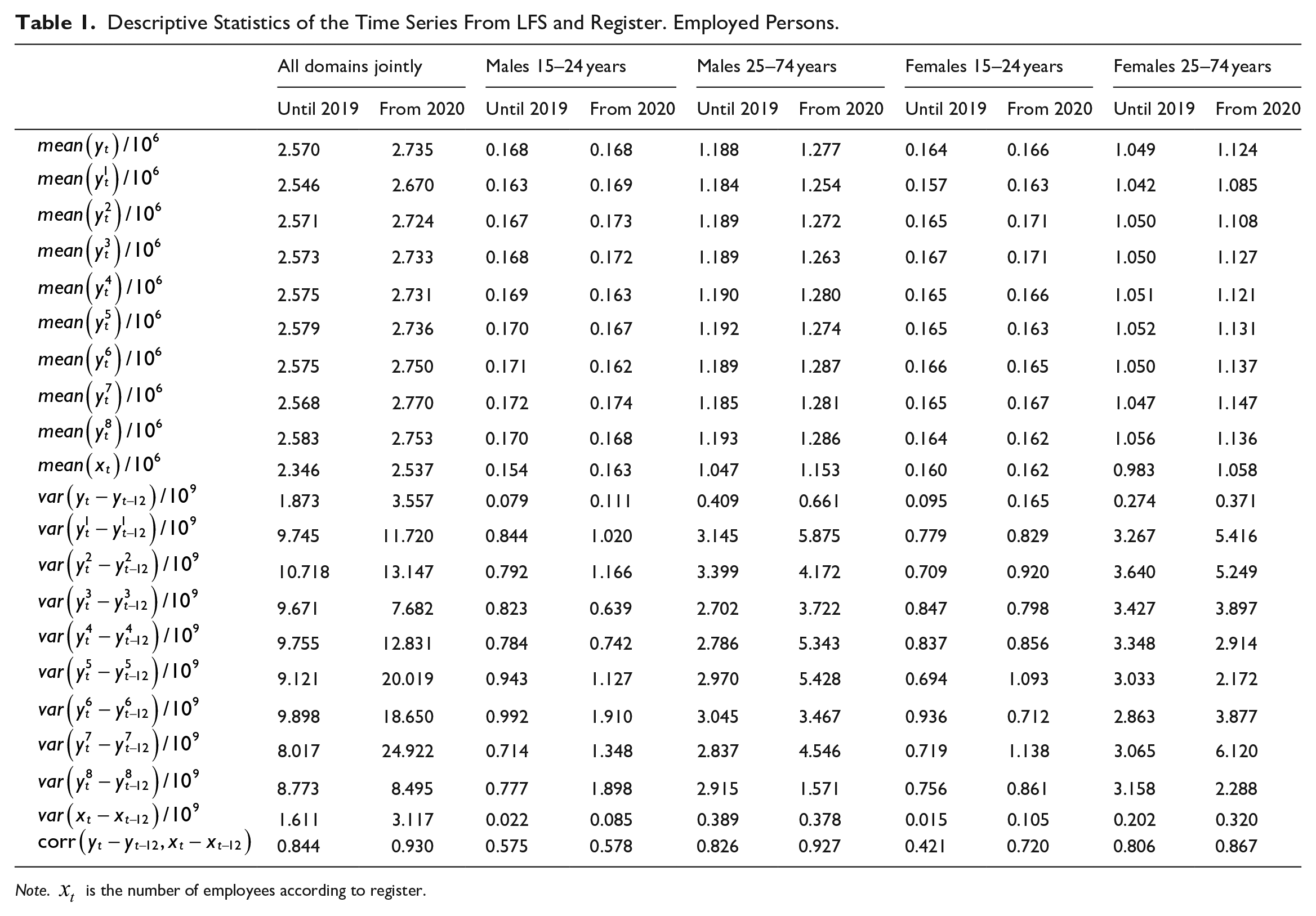
Descriptive Statistics of the Time Series From LFS and Register. Employed Persons.
Note.
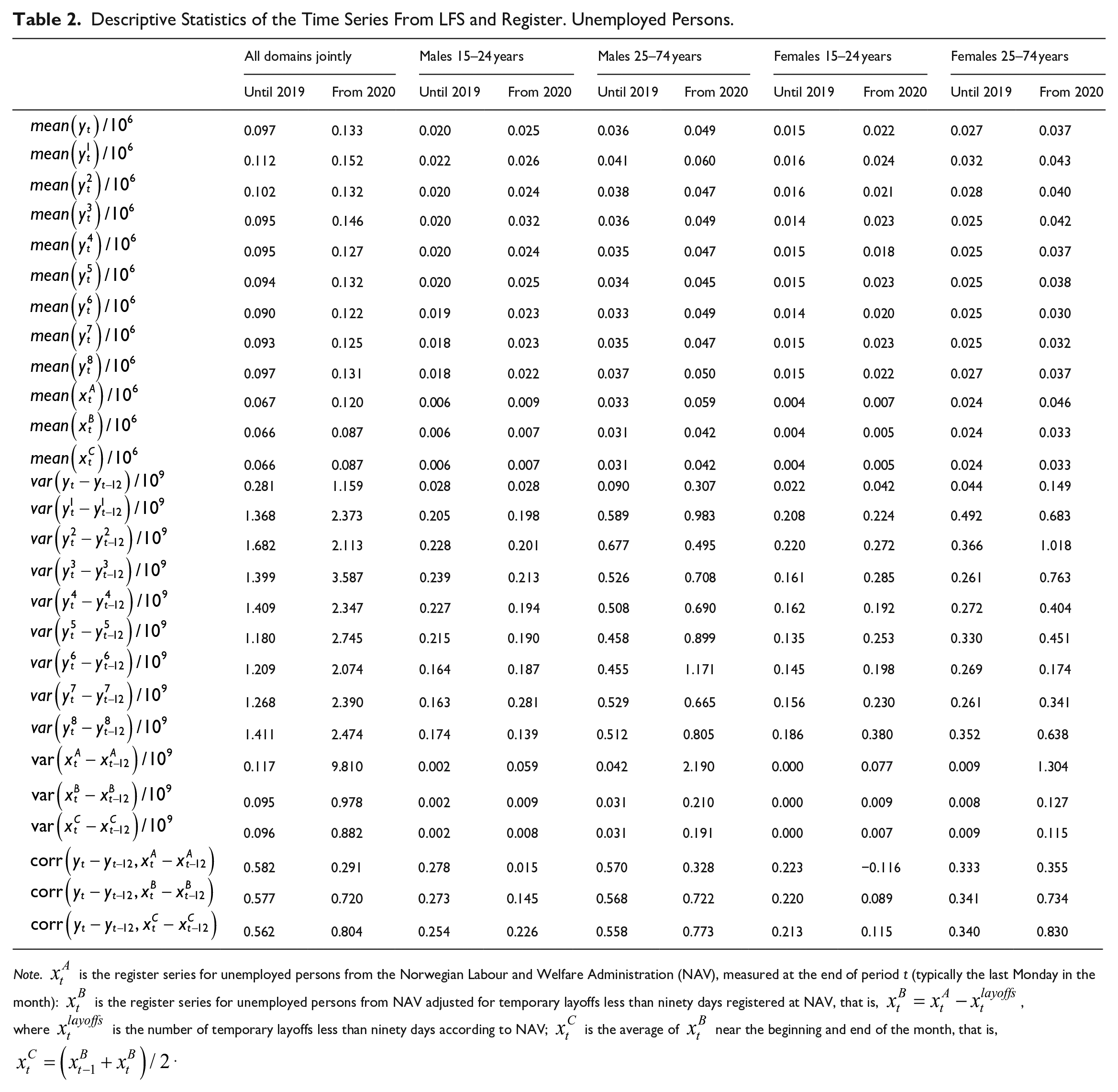
Descriptive Statistics of the Time Series From LFS and Register. Unemployed Persons.
Note.
2.1. The Norwegian LFS
LFS measures key labor market indicators in the population, such as employment and unemployment. In our observation period, data collection has been carried out by means of telephone interviews only.
The Norwegian LFS has a rotating panel design. Since 1996, participants have been requested to respond every three months for a total of eight consecutive quarters. In each quarter, 1/8 of the sample leaves the survey after finishing the last wave, and an equivalent number of new interviewees are included for the first time. First-time interviewees constitute wave 1, those interviewed for the second time wave 2, and so on. Those interviewed for the last time are thus those in wave 8. The sample size in the survey is around 24,000 persons per quarter.
The nonresponse rate in the Norwegian LFS varied from 14 to 21% in the years 2016 to 2020, see Eurostat (2022), and the response rates are almost the same for all waves. Eurostat (2022, Table 4.5) reports nonresponse rates of the member states of the European Union, three EFTA countries (including Norway) and four candidate countries. The rates are not comparable as the magnitude of nonresponse is based on household units for most countries. For Norway, like Denmark, Estonia, Luxembourg, Finland, Sweden, Iceland, and Switzerland, the figures are for nonresponse at an individual level. Of these countries, Norway has the lowest nonresponse rate, while Switzerland has the second-lowest nonresponse rate at around 20%. The majority of other countries that calculate the nonresponse rate in the same way as Norway have nonresponse rates of 30 to 50%.
Before 2021, the sampling unit was the core family. The core family consists of married couples and registered same-sex couples with their children, and single-parents with children. Other units were considered to be single-person families. In this period, the survey used a stratified, one-stage cluster design. Individuals were clustered into family units, and the sample was stratified using geographical areas. The interviewees are the persons in the age group 15 to 74 in these families, and each of them is interviewed.
The responses from the LFS participants are assigned weights based on how representative they are for the total population. These weights are assigned to the individual person (not the sampled family) and used to estimate the LFS variables. The estimation procedure for the Norwegian LFS is a one-step multiple-model calibration based on monthly LFS and register data. The method uses register data for employment status, age, sex, NUTS2 region, immigration background, education level, family size, and marital status. The method is described further in Oguz-Alper (2018); see also Nguyen and Zhang (2020).
Let
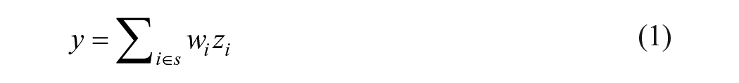
where we have omitted subscripts for time and domain for all variables to simplify the notation, and s represents the set of persons that have responded to the survey.
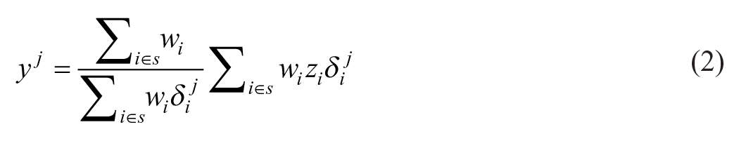
We apply the same weights as for the overall estimates to generate the wave-specific estimates for employment and unemployment used in this analysis. Let
The first line in Table 1 reports the mean of the number of employed persons according to the LFS given by Equation (1) for two subperiods, that is, for the period 2006M1-2019M12 and the remaining sample period 2020M1-2021M10, as we suspect the variances to be significantly higher in the second subperiod due to the presence of the COVID-19 pandemic. We also provide estimates for four domains. These domains are based on two age groups for both sexes. We distinguish between young persons aged 15 to 24 years and persons aged 25 to 74 years, which is an age classification used by both Eurostat and Statistics Norway. Most of the employed individuals of both sexes are in the “older” age group.
Similarly, the first line in Table 2 reports the mean value of unemployed persons given by Equation (1) for the same time periods and domains that are as used in Table 1. When considering the estimates of unemployment according to the LFS, we also see that most are in the oldest age groups. However, the unemployed are more evenly distributed amongst the groups than the employed. Thus, the unemployment rate, which is not reported in the table, is lower for the “older” age groups.
Tables 1 and 2 also report the mean value of the wave-specific estimates according to Equation (2). The wave-specific estimate is especially pronounced for wave 1 for all domains, with lower employment and higher unemployment than the average.
In the lower parts of Tables 1 and 2, we report the empirical variance of the twelve-month growth in employment and unemployment according to the LFS for each wave and for the mean of the waves. The variance for a specific wave is substantially larger than the variance of the mean of the waves. As noted for the means above, the variances of the register variables are less than those of the LFS variables.
2.2. The Most Important Changes in the 2021- Redesign of the Norwegian LFS
In the beginning of 2021, some changes were made in the Norwegian LFS. The main reason for the restructuring is the new EU regulation. The changes are intended to improve the quality of statistics, increase compar ability across countries, and across domains in social statistics. Therefore, a similar restructuring of the LFS has taken place in all EU and associated countries. The sampling design was also changed in the Norwegian LFS, even though this was not a requirement from Eurostat. From 2021, the sampling unit was changed from core family to individual persons, and the population is stratified by combinations of region, age-group, and register-based employment status; see Jentoft (2022) for details. The direct estimates in Equations (1) and (2) still apply, where the weights are based on basically the same estimation procedure as before 2021; see Oguz-Alper (2023) for details.
The redesign also means that the target population was changed from covering all registered residents aged 15 to 74 to registered residents aged 15 to 89 in private households. This means that more age groups are included in the survey, but also that some persons are excluded from the target populations as they do not live in private households. The most important examples of the latter are persons enrolled in compulsory military service and persons registered as residents in institutions. Until the beginning of 2021, persons in the same family could answer for other family members. Due to the change of the sampling unit to individual person, Statistics Norway has stopped using such proxy interviewing. This change may have led to higher nonresponse, especially from younger persons, but this should at least partly be compensated for by weighting as the weights are calibrated on, among other variables, detailed age groups and register-based employment status. See Zhang et al. (2013) for a discussion of proxy interviewing in the Norwegian LFS and reduction of nonresponse bias through weighting when good auxiliary register variables are available.
In the new questionnaire, question sequences, formulations and response options have changed due to modernisation of the language, increased international coordination, and adapted self-reporting as a future data collection method.
The alternative to an immediate introduction of a new questionnaire in January 2021 would be a gradual introduction. Such a gradual introduction of the new questionnaire was done in the Netherlands, see Van den Brakel (2022). The advantage of a gradual phasing in of the new questionnaire is that one can get better estimates of the structural break, since one can compare changes in waves where the questionnaire is changed with waves where the questionnaire is not changed. But this means that both new and old LFS questionnaires are used during a transition period, and systems must be in place that can handle a double set of questionnaires. Statistics Norway therefore chose to change the questionnaires for all waves at the same time.
Before 2021, individuals regarded as temporary layoffs for more than ninety days were automatically considered unemployed in the Norwegian LFS without being asked about active job search or availability. From 2021 on, temporary layoffs for more than ninety days will get the usual questions about job search and availability in the LFS, thus potentially being classified as outside the labor force. This change in the questionnaire, combined with the fact that the Norwegian labor market at the same time was facing a situation with many temporary layoffs in connection with the COVID-19 pandemic, could reduce the number of unemployed when the new LFS design replaces the old one.
2.3. Register Data, Harmonization and Pre-Adjustment for Earlier Structural Breaks
In the time series model for employed persons according to the LFS we utilize a time series for the number of registered employees in the domain. Similarly, the time series model for LFS unemployment in a domain utilizes an auxiliary register time series for that domain from the unemployed registered at the employment office (registered unemployment). The auxiliary register variable in time series models needs to be comparable over time and should not include structural breaks, at least not at the same time as the 2021 redesign.
With respect to the LFS employment model, for the period before 2015, we use register information from the Register of Employers and Employees. In January 2015, the Register of Employers and Employees was replaced by the new a-scheme register for monthly reporting of employee and payroll information to the Norwegian Labour and Welfare Administration (NAV), the Norwegian Tax Administration and Statistics Norway. Since the auxiliary variable is based on two different sources of information in the start and the end of the sample, brought about by the transition from the Register of Employers and Employees to the new a-scheme register, it has been corrected for changed level and seasonal patterns (see also Part B of our Supplemental Documentation).
From Table 1 we see that there is a high correlation between the development in LFS employment and registered employment. This correlation has been particularly high since 2020, with a correlation coefficient of 93% for the full sample. The correlation coefficients for the domains are somewhat lower but still exceed 80% for the “older” domains for both males and females. For young males, the correlation coefficient is about 60%, and for young females, about 70%.
In the model for unemployment, we use estimates for persons registered by NAV as unemployed. In contrast to the LFS estimates, in the register from NAV, temporary layoffs are regarded as unemployed from the first day. Due to different treatment of temporary layoffs, there is a large discrepancy in the observed relationship between LFS unemployed and the official registered unemployed estimates for the first couple of months of the COVID-19 pandemic in Norway, starting in March 2020. Therefore, “layoff-harmonized” registered unemployed estimates have been constructed by excluding temporary layoffs from the official NAV figures in the first three months. This harmonization brings the definition more into line with the definition of LFS unemployment because the LFS treat temporary layoffs as employed temporarily absent for the first ninety days. This harmonization of the register variables is designed to bring about a higher correlation between the growth in the register and LFS variables.
The official NAV unemployment estimates indicate the number of registered unemployed close to the end of the month. For our auxiliary register variable to be more representative of the monthly average of unemployed according to the LFS, we use the average of the auxiliary register variables observed close to the end of the month in question and the end of the previous month. This averaging of our pre-adjusted harmonized register unemployment variable is vital in months with large changes in unemployment, such as for the start of the initial shutdown period of the COVID-19 pandemic in Norway in March 2020.
Table 2 reveals the advantages of our adjustments of the registered unemployment series. When observations from 2020M1 till 2021M10 are considered for all domains together, the twelve-month growth in official NAV unemployment series shows a correlation of 29.1% with the growth in the corresponding LFS series. This correlation coefficient increases to 72.0% when we adjust for layoffs. When this adjusted unemployment according to register is measured as a two-month average, the correlation coefficient increases even further, to 80.4%. We see the same pattern for all domains. Due to our adjustments, the correlation coefficient for “older” males increases from 32.8 to 77.3%. The correlation for “older” females increases from 35.5 to 83.0%. For young males and females, the correlation between the register variables and the LFS variables is appreciably smaller. However, our adjustments increase the correlation for these domains, too.
2.4. Information From Parallel Data Collection in 2020Q4
The results of a parallel data collection may help in a time series model to produce more precise estimates of the effect due to redesigning a survey. In the last quarter of 2020, a sample of 2,626 persons were interviewed using the new questionnaire. The persons in this extra sample were only interviewed once. The results of these interviews can be compared with the results from wave 1 of the ordinary LFS interviews when using the old questionnaire. This will give an estimate of the structural break for wave 1 together with an estimate of its variance.
The extra sample is too small for the effects of the 2021 redesign to be estimated precisely. However, the information can still be combined with a time series model to model the effects of the 2021 LFS redesign. This approach is discussed in Van den Brakel et al. (2020). Because the sample is small, we cannot use the usual calibration model. Therefore, a simplified version of the calibration model is used for deriving weights. A more detailed description of the parallel survey and this calibration model is given in Part G of the Supplemental Documentation.
3. Time Series Model for Estimating Possible Overall Structural Breaks Due to the 2021 LFS-Redesign
In Subsection 3.1, we outline the basic model for the Norwegian LFS. Subsection 3.2 presents our first contribution, which is the symmetric treatment of wave-specific effects. In Subsection 3.3, the model is extended to include a structural break and an auxiliary variable. The article’s second contribution is presented in Subsection 3.4, where we allow for a time-varying hyperparameter for the trends for both the LFS variables and the auxiliary variables in order to account for the substantial fluctuations in the labor force during the pandemic when estimating the structural break.
3.1. The Basic State-Space Model of the Norwegian LFS
In this section, we reasonably assume that all eight waves follow the same trend, have the same seasonal pattern and irregularities, and have an autocorrelated survey error component because of the rotating design. Pfeffermann (1991) derives a model for such a repeated survey.
We define

where

where
The trend is generally assumed to follow a local level model, a local linear trend model, or a smooth trend model; see for example, Harvey (1989) and Durbin and Koopman (2012). We follow Van den Brakel and Krieg (2009) and apply the smooth trend model

where
The seasonal component,
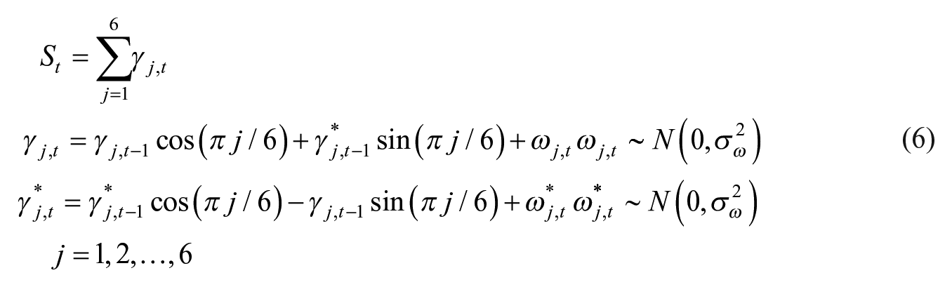
The first frequency of π/6, that is, the fundamental frequency, corresponds to a period of twelve months, whereas the five other frequencies are harmonics. We note that this process depends on only one hyperparameter, as the variance
The irregular component
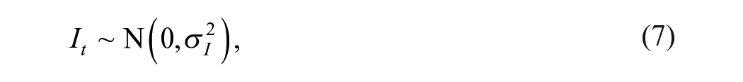
where
The interviewees in the first wave are interviewed for the first time, whereas the interviewees in the other waves have been interviewed before. The variance of the wave-specific survey errors is also time-dependent, partly due to variation in the number of persons interviewed each month; see Binder and Dick (1990) and Van den Brakel and Krieg (2009). Let


If
Based on Equation (2) and assuming equal weights, we apply a rough approximate estimate of the variance of survey error for the wave-specific monthly LFS-estimates given by
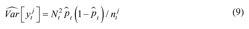
as an estimate for the square of
The autocorrelation coefficient in Equation (8),
3.2. Symmetric Treatment of the Wave-Specific Effects
Investigating the responses from the US current population survey (which corresponds to the LFS in many other countries), Bailar (1975) shows that the number of persons reporting as unemployed is much higher for those participating in the survey for the first time. Similar results for the US current population survey are also found in Stephan et al. (1954, A-80) and Hansen et al. (1955, 710), and in Kumar and Lee (1983) for the Canadian LFS. Pfeffermann (1991) takes account of this in his model for repeated surveys by including wave-specific effects. However, the model only takes account of time-invariant wave-specific effects (although he mentions that the model can be extended to allow for time-varying wave-specific effects). Van den Brakel and Krieg (2009) extend the model to include time-varying wave-specific effects.
For both the trend component in
In contrast, we apply the restriction
The restriction
To avoid the process of one of the wave-specific effects having a higher variance than the other, we apply a symmetric approach;
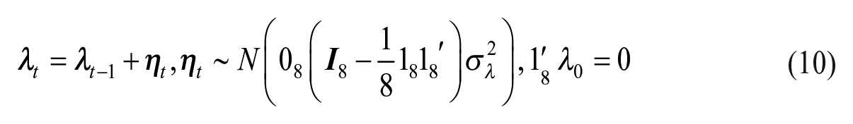
where
The specification of the wave-specific effects in Equation (10) might not be easy to implement in a software program for state-space models. The restriction
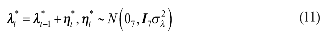
Note that if we premultiply (11) with
To derive
3.3. Structural Break and Auxiliary Variables
We now extend our model to allow for a possible structural break following Harvey and Durbin (1986). When a structural break is included, (3) changes to

In Equation (12),
Without a gradual phasing in of the new questionnaire, the use of auxiliary variables become even more important. We include auxiliary variables in the models to get a better grasp on quantifying the structural breaks. If

where
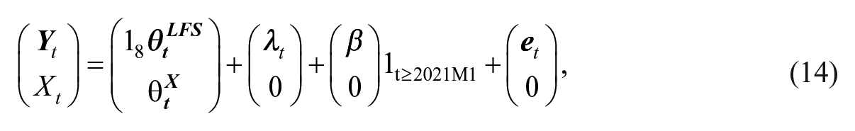
where the superscript LFS is included to emphasize that these latent processes and parameters are related to the LFS.
For it to be advantageous to model the LFS variables (LFS unemployment or LFS employment) and the register variable jointly, there must be a correlation between them. Therefore, we allow the disturbance terms of the trend slope components of the LFS variables and the auxiliary variable, the X-variable, to be correlated. The covariance between the disturbance terms of the slopes of LFS variable trend and the register variable trend is given by

where
3.4. Larger Fluctuation in the Trend During COVID-19
The COVID-19 pandemic led to large fluctuations in the labor market. The model we have outlined above does not allow for larger fluctuations in the labor market during the pandemic. The structural break estimates may be severely biased if this increased variation in the LFS and register time series is neglected.
In the Netherlands, the Labor Force Survey estimates are improved by applying a state-space model; see Van den Brakel and Krieg (2009). During the COVID-19 pandemic, they had to modify the state-space model to account for the more rapid changes in the labor market; see Van den Brakel et al. (2022). They did so by allowing for a time-varying hyperparameter for the slope of the trend. Gonçalves et al. (2022) applied the same approach for the LFS in Brazil. However, neither Van den Brakel et al. (2022) nor Gonçalves et al. (2022) considered to include an auxiliary variable. Bollineni-Balabay et al. (2016) applied a similar approach when considering both level and variance breaks due to survey redesign. However, they did not include an auxiliary variable. Here, we use similar modeling of both the LFS and the register trend.

The specification in Equation (16) implies that the slope-variance hyperparameter is time-varying and given by
We have divided our sample into three parts. The first is the pre-corona part, defined as the period up to and including 2019M12. In this period, we apply
3.5. Estimation and Statistical Inference
We cast our (parsimonious) models in state-space form and estimate their hyperparameters by maximizing the diffuse log-likelihood function using the BFGS algorithm. The formal specification of the state-space model with all the underlying assumptions is given in the Appendix (Subsection 6.2). Special features of our state-space models are that there are no measurement errors in the measurement (vector) equation, the transition matrices are always time-invariant, and the selection matrices of the transition equations are potentially time-varying, see also the Appendix (Subsection 6.2). The main purpose of our article is to investigate whether the redesign of the LFS survey impacts employment and unemployment. The intervention effects are assumed to be wave-specific and constant. Technically, they are represented by elements in the state vector that are without disturbances.
An essential part of the estimation algorithm is to run the Kalman filter during the recursions in order to update the state vector estimate. KFAS, see Helske (2017), utilizes a complete univariate approach for filtering and smoothing provided by Koopman and Durbin (2003); see also Anderson and Moore (1979) for sequential processing. This constitutes a way of implementing so-called exact diffuse initialization. Such a procedure makes the results less prone to numerical error than when uninformative diffuse priors are used. An important aspect of our study is to compare model specifications with time-invariant hyperparameters with model specifications that allow for time-varying hyperparameters. To this end, we use likelihood ratio tests.
After obtaining the maximum likelihood estimates of our unknown hyperparameters, we obtain (final) smoothed estimates of the state vectors. Diagnostics of the state space model can be constructed from the standardized one-step-ahead prediction errors.
4. Empirical Results
This section presents the estimated hyperparameters and the structural break estimates due to the 2021 LFS-redesign. The models are estimated on monthly data from 2006M1 to 2021M10. Apart from the pre-estimation of the autocorrelation parameters related to the survey error component, all other inference has been carried out using the R package KFAS, see Helske (2017).
Following Pfeffermann et al. (1998), we estimate the autocorrelation coefficient of the survey errors in a separate system; see the Appendix (Subsection 6.1). By doing so, we can treat the coefficient as “known” when estimating the remaining parameters of the state-space model. We also apply a grid search to estimate
4.1. Estimated Hyperparameters and Other Results
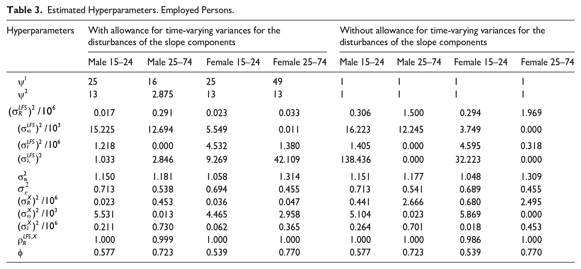
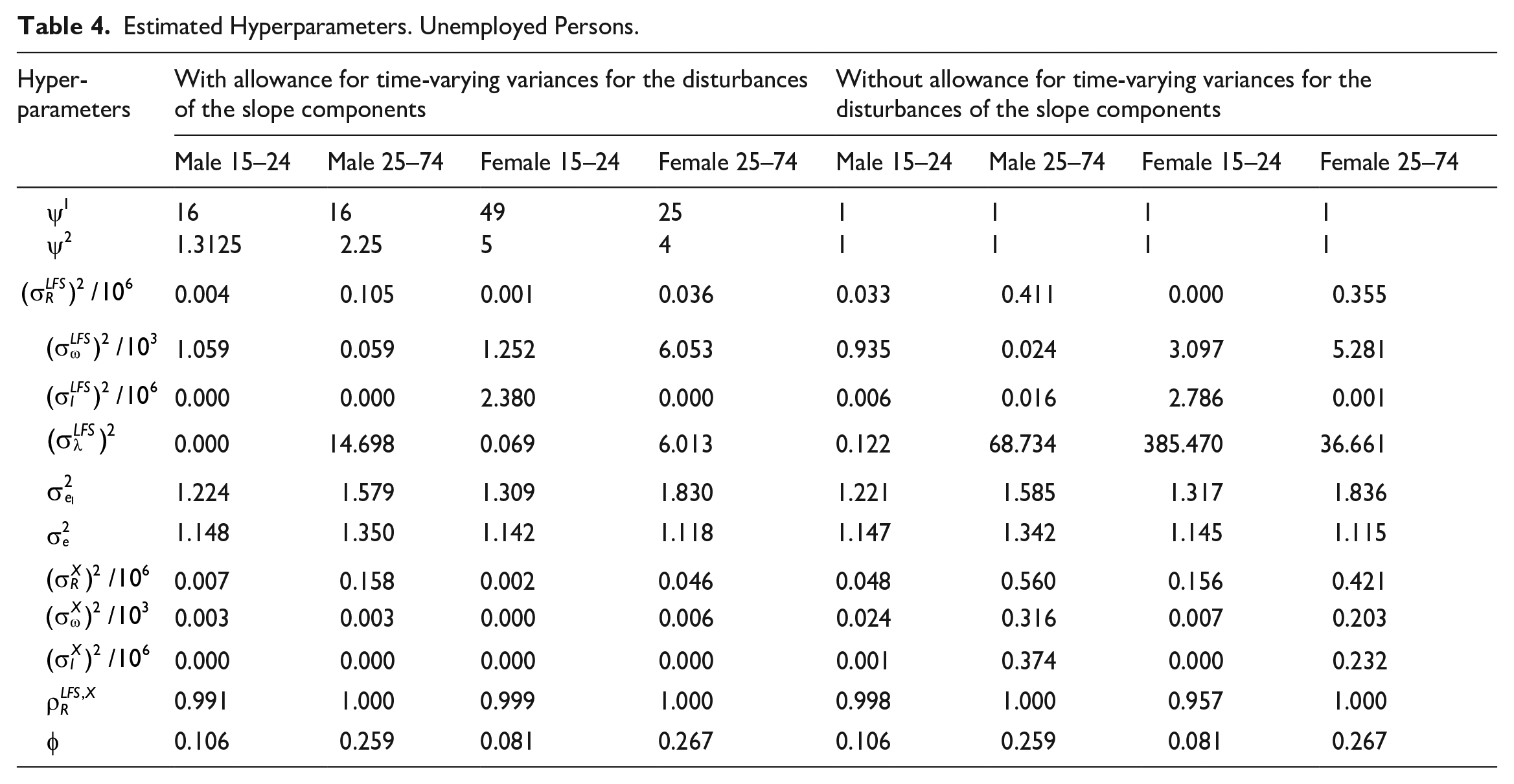
Tables 3 and 4 provide an overview of the maximum likelihood estimates of the hyperparameters for employment and unemployment, respectively. In the tables, we consider both the case with estimated parameters
Estimated Hyperparameters. Employed Persons.
Estimated Hyperparameters. Unemployed Persons.
The estimate of
For all the domains of employment, the estimate of the hyperparameter for the slope of the trend,
Tables 3 and 4 also reveal a high correlation between the disturbances of the slope of the LFS trend and the register trend. For all domains, the estimated correlation between the disturbances of the two trend-slopes is equal or very close to 1. This strong correlation is advantageous for estimating possible structural breaks due to the 2021 LFS-redesign. A correlation equal to 1 implies that the LFS-variables and the register variable follow a common stochastic trend and are thus cointegrated; see Engle and Granger (1987).
In the bottom line of Tables 3 and 4, we report the estimate of autocorrelation parameter of the survey errors,
Diagnostics related to the behavior of the disturbances in the state vector can be derived from the one-step-ahead standardized prediction errors. (In Part E of our Supplemental Documentation, we report some diagnostics based on the one-step-ahead prediction errors and some graphs based on these errors and auxiliary residuals.) The standardized innovations seem to be reasonably well-behaved, although a part of the test diagnostics for some of the waves are significant at the 5% test level. With respect to the auxiliary residuals, Harvey and Koopman (1992) show these to be useful for detecting outliers and structural changes. Auxiliary residuals are smoothed estimates of the disturbances associated with the unobserved components. In the case with time-varying hyperparameters, the auxiliary residuals seem to perform better during the years 2020 and 2021 than in the case with time-invariant hyperparameters; see Part I in the Supplemental Documentation. We interpret this as evidence that our specification of the stepwise shifts in the variances of the disturbances of the slope components of the trends captures quite well the excess residual fluctuations in the last part of the sample that are present in the case with time-invariant hyperparameters.
Tables 3 and 4 also reveal that the estimated hyperparameters of the wave-specific effects are small. With such low values, imposing time-independent wave-specific effects (which occur when these hyperparameters are zero) would presumably have been innocent. Thus, in this case, the symmetric specification of the time-varying wave-specific effects is probably not that important in order to obtain a precise estimate of the structural break.
4.2. Structural Break Estimates
Table 5 reports the structural break estimates for employment in the four domains both when we allow for time-varying hyperparameters and when we do not. For comparison, we also report a column with the number of employed persons in 2019, the year before the COVID-19 pandemic, according to the LFS. When considering each wave separately, there is considerable uncertainty in the structural break estimates. Therefore, the domain-specific structural break estimates are given as the average of the estimates of the structural break parameters for the eight waves. The estimated total effect of the structural break in employment is 21,864 persons when we allow for time-varying hyperparameters and 24,307 when we do not. Measured relative to employment according to the LFS in 2019, the estimated structural break constitutes about 0.8 to 0.9% of employment and 0.6% of the population. From the table, we see that it is the structural break estimate for males aged 25 to 74 that is most affected by allowing for a time-varying hyperparameter: When assuming time-invariant hyperparameters, we obtain a structural break estimate for this domain of 5,002 persons, but this estimate changes to −381 when allowance is made for time-varying hyperparameters for the disturbances of the slopes. The structural break estimate for young females also changes when allowance is made for time-varying hyperparameters, from 5,442 to 8,115. The difference in the break estimate in the two specifications (with and without time-varying hyperparameters) is still relatively small when we compare it with the number of employees in these two domains. The difference in the break estimate for males aged 25 to 74 was 5,383, which corresponds to 0.4% of the number of employed in this domain in 2019. And the difference in the break estimate for females aged 15 to 24 corresponds to 1.6% of the number of employees in this domain.
Structural Break Estimates for Employed Persons, by Sex and Age. a
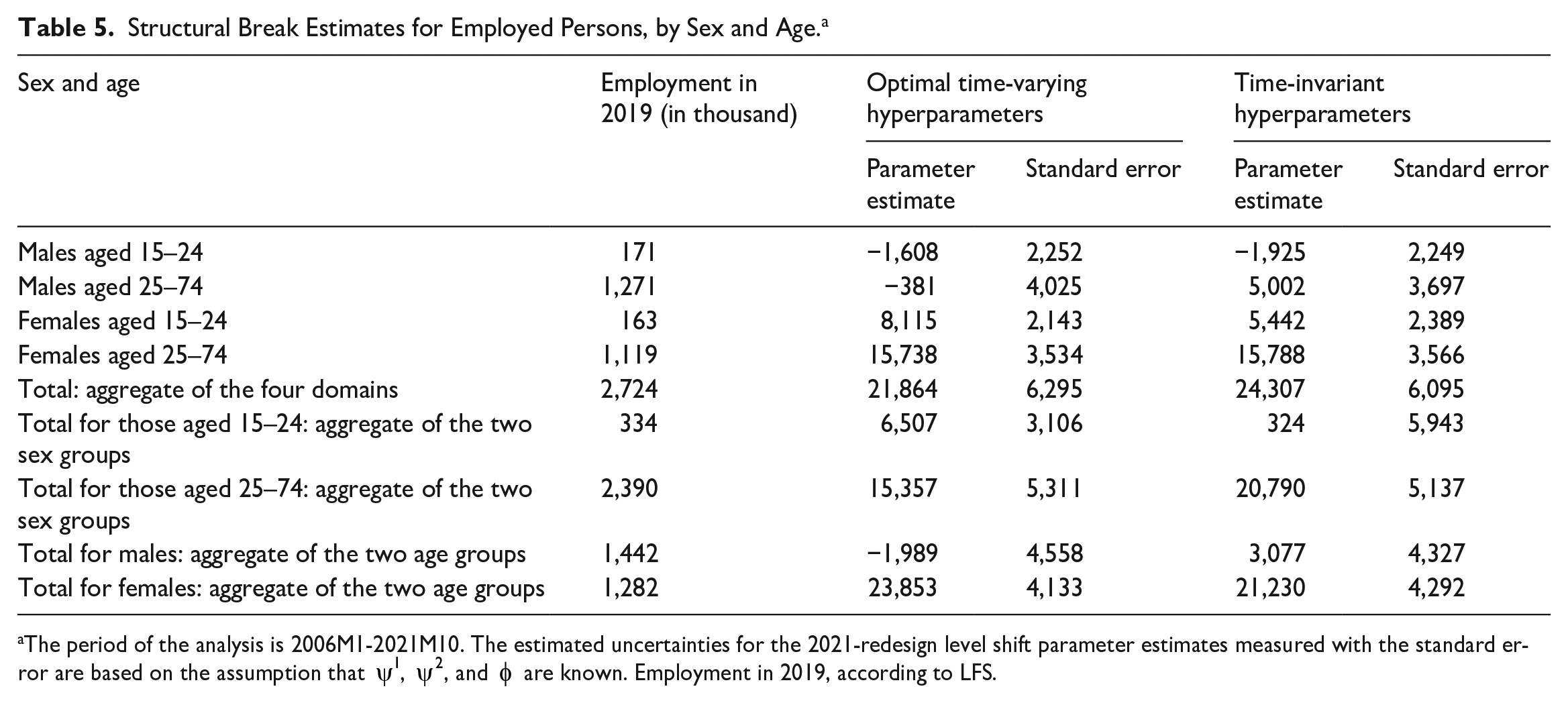
The period of the analysis is 2006M1-2021M10. The estimated uncertainties for the 2021-redesign level shift parameter estimates measured with the standard error are based on the assumption that
When time-varying variances for the disturbances of the slopes are allowed for, the structural break estimates for males are small and insignificant when measured either individually or jointly. The estimates for women are all positive and significant. Thus, our analysis implies that the redesign of the Norwegian LFS led to an increase in measured employment for women.
Table 6 reports estimates of the structural break for unemployment in the four domains. For comparison, we also report a column with the number of unemployed persons in 2019 according to the LFS. When the hyperparameters of the disturbances of the two trend slopes are allowed to be time-varying, the total estimated effect of the structural break on unemployment figures is 5,371. This corresponds to 5.1% of the LFS unemployment in 2019, but just 0.1% of the population. When the hyperparameters related to the slopes are assumed to be time-invariant for all domains, the estimated total effect of the structural break is 7,841 persons, or 7.4% of the LFS unemployment in 2019 (and about 0.2% of the LFS population). The estimates for unemployed females are virtually unaltered by allowing for time-varying hyperparameters. Therefore, the change in the total structural break estimate when allowance is made for time-varying hyperparameters of the slopes is due to the change in the estimates for males. The overall structural break estimate for males is reduced by more than 2,000 persons (from 3,847 to 1,723) when time-varying variances are allowed for the disturbances of the trend slopes.
Structural Break Estimates for Unemployed Persons, by Sex and Age. a
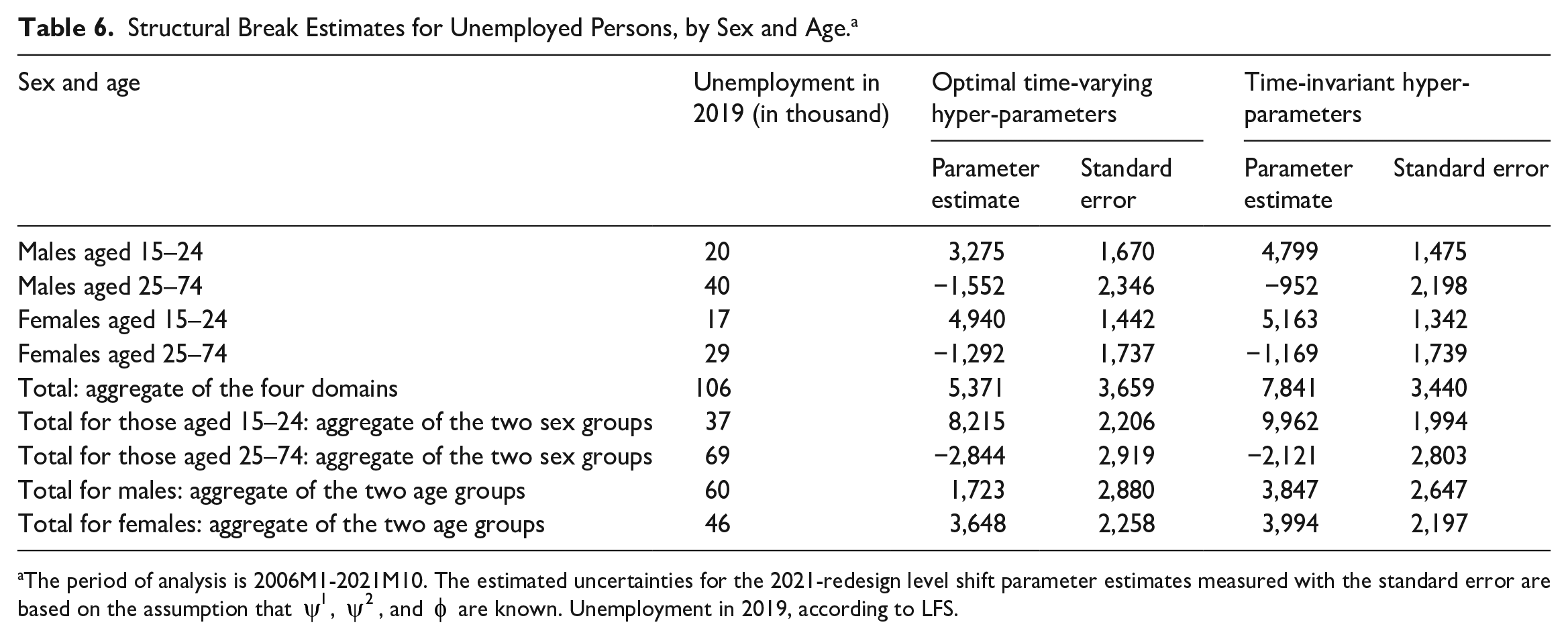
The period of analysis is 2006M1-2021M10. The estimated uncertainties for the 2021-redesign level shift parameter estimates measured with the standard error are based on the assumption that
Only ten months of observations of the LFS after the redesign may be too few to estimate the structural breaks precisely. In Part F of the Supplemental Documentation, recursive break estimates are therefore reported, that is, the break estimate with only one month of observation after the redesign, the break estimate with two months of data after the redesign, and so on. For most of the domains, it seems that the break estimate has converged. However, this is not the case for the break estimate for employment among young men, where the estimate is adjusted by over 2,000 persons when the figures for 2021M10 are included. The break estimate is nevertheless non-significant.
5. Conclusions
In 2021, the Norwegian LFS underwent a substantial redesign in accordance with the new regulation for integrated European social statistics. To ensure coherent labor market time series for the main indicators, the redesign’s impact is modeled. The estimated structural breaks can be used to adjust the previously published LFS series prior to 2021 such that they are comparable to the LFS figures after the redesign. The adjustment can be made by revising the historical figures corresponding to the estimated structural break, or by scaling the break with relative changes in the population for the individual domain. Statistics Norway has chosen the latter approach.
In this article, we have pursued a structural time series approach in the tradition of Pfeffermann (1991), Van den Brakel and Krieg (2009, 2015), and Elliott and Zong (2019). Structural breaks were estimated for the numbers of employed and unemployed persons in different domains.
We obtained a structural break estimate of about 22,000 employed and 5,000 unemployed persons aged 15 to 74 when allowing for time-varying hyperparameters for the disturbances of the slopes of the two trend variables. When no such allowance was made, the estimated breaks for employment and unemployment were about 2,000 to 3,000 higher. Both likelihood ratio tests and examination of the auxiliary residuals indicate that the hyperparameters related to the slopes are time-varying with higher values during the COVID-19 pandemic.
The structural break estimates identified for Norway are of the same sign as found in the Netherlands; see Van den Brakel (2022). However, our estimates are much smaller. Van den Brakel (2022) identifies a structural break estimate in employment that corresponds to more than 1.5% of the population in the LFS, and a structural break estimate in unemployment that exceeds 1% of the population. For Norway, the estimates of the structural break imply a positive shift in the employment figure of slightly less than 0.6% and for unemployment of just over 0.1%, measured in relation to the LFS population.
In the analysis, we have followed Van den Brakel and Krieg (2015) and Gonçalves et al. (2022), among others, by only allowing correlation between the disturbances of the slope of the trend component of the LFS variable and the trend component of the register variable. We could have extended this specification by also allowing for correlations between the disturbances of the seasonal components and between the disturbances of the irregular components; see, for example, Van den Brakel and Krieg (2016) for specifying such correlations between domains. Elliott and Zong (2019) allow for correlation between the disturbances of the three common components across the LFS and the register from the outset but end up with a specification which only includes a correlation between the disturbances of the two trend components.
Four different domains are considered in this analysis. However, we have not considered correlations between these domains. Allowing correlations between domains implies borrowing strength between domains. Pfeffermann and Burck (1990), Rao and Yu (1994), Datta et al. (1999), Pfeffermann and Tiller (2006), Boonstra and Van den Brakel (2022), among others, have considered such correlations between domains.
In this analysis, we assumed that only one break is taking place in all waves simultaneously. However, there could be delayed effects of the new sampling system as each quarter after the beginning of 2021, a new wave is included according to the new sample design. The first quarter where all waves have only been subject to the new sampling system is 2022Q4. We would have needed at least one more year of observations to analyze this possible delayed effect. Therefore, such effects were not feasible to estimate with our data set. However, investigating such delayed effects could be interesting for a follow-up analysis. The new LFS-design could also lead to a structural break in the seasonal pattern. To analyze such possible structural break in the seasonal pattern, longer data series would have been needed.
Supplemental Material
sj-pdf-1-jof-10.1177_0282423X241235267 – Supplemental material for Structural Break in the Norwegian Labor Force Survey Due to a Redesign During a Pandemic
Supplemental material, sj-pdf-1-jof-10.1177_0282423X241235267 for Structural Break in the Norwegian Labor Force Survey Due to a Redesign During a Pandemic by Håvard Hungnes, Terje Skjerpen, Jørn Ivar Hamre, Xiaoming Chen Jansen, Dinh Quang Pham, and Ole Sandvik in Journal of Official Statistics
Footnotes
6. Appendix
Acknowledgements
We would like to thank the associated editor and the referees for constructive comments and suggestions. Furthermore, we thank Susie Jentoft, Melike Oguz-Alper, Arvid Raknerud, and Ole Villund for valuable comments. Many thanks also to Jan van den Brakel who visited Statistics Norway in February 2020 and gave a course in time series analysis of survey redesigns. Any remaining errors and shortcomings are the sole responsibility of the authors.
Funding
The author(s) disclosed receipt of the following financial support for the research, authorship, and/or publication of this article: Eurostat partially funded this article under grant agreement: 826605—2018-NO-LFS-QUALITY BREAKS.
Supplemental Material
Supplemental material for this article is available online.
Received: August 2022
Accepted: October 2023
References
Supplementary Material
Please find the following supplemental material available below.
For Open Access articles published under a Creative Commons License, all supplemental material carries the same license as the article it is associated with.
For non-Open Access articles published, all supplemental material carries a non-exclusive license, and permission requests for re-use of supplemental material or any part of supplemental material shall be sent directly to the copyright owner as specified in the copyright notice associated with the article.