Nonresponse Bias of Japanese Wage Statistics

Abstract

This article analyzes unit nonresponse bias of establishment surveys, drawing on two major government wage surveys in Japan. We find that unit nonresponse is prevalent among establishments with fewer employees, in urban prefectures, and operating in the service industry. Further, while low-wage establishments are less likely to respond, the resulting bias is quantitatively negligible. Regarding establishment sampling of employees, we find that the sampled establishments randomly choose workers in an appropriate manner. Overall, with proper weighting, nonresponse bias is negligible in Japanese wage statistics to the extent that the mean estimate is concerned. In addition to nonresponse bias, we also assess potential bias due to limited coverage of the sampling population and find substantial bias at the tails of the wage distribution. In particular, excluding corporate executives and establishments with few employees results in an underestimation of wage inequality.

1. Introduction

Wage statistics play a crucial role in policymaking by providing one of the most important signals for monitoring the current state of the economy. For example, changes in nominal wages are regularly cited in Bank of Japan quarterly publications such as “The Outlook for Economic Activity and Prices of the Bank of Japan” which provide background information for monetary policy meetings and insight into its monetary policy stance. The government also uses wage statistics for administrative purposes such as wage inflation adjustments of unemployment benefits and worker compensation for occupational injury. Researchers, too, use wage statistics to analyze topics ranging from the impact of minimum wages to macroeconomic wage dynamics (Hoshi and Kashyap 2021; Kawaguchi and Mori 2021). Given the importance of wage statistics for both policymakers and researchers, the long-term declining trend in response rates for government surveys which is common across developed countries raises questions about the representativeness of wage statistics. Yet despite heightened attention to the possibility of nonresponse bias, there has been little systematic assessment of the method by which wage statistics are collected in Japan.

Studies of nonresponse bias in earnings surveys, based mainly on the US Current Population Survey (CPS), have set an important path for investigating the issue. Nonresponse bias is ignorable if the survey response behavior is characterized by observable characteristics, as the population distribution can be recovered by applying appropriate weights. On the other hand, nonresponse bias is non-ignorable if the survey response behavior depends on unobserved determinants of the outcome variable. In this latter case, recovering the population distribution from the sample becomes difficult unless there exists a credible instrumental variable that affects the response behavior but does not affect the outcome variable. In this study, we analyze the dependence of response behavior on both observed and unobserved characteristics.

For our investigation of the validity of wage statistics in Japan, we examined two large-scale surveys that are conducted independently by two different national government ministries. These are the Basic Survey on Wage Structure (BSWS) by the Ministry of Health, Welfare and Labour, and the Statistical Survey of Actual Status for Salary in the Private Sector (SSPS) by the National Tax Agency. We assessed their quality in terms of their representativeness of the population and the quality of their wage measurements. Both the BSWS and SSPS collect the wage information of individual workers through establishment surveys drawing on a similar two-stage sampling design. In the first stage, the survey administrator randomly selects establishments according to the stratified sampling method. In the second stage, the administrator instructs personnel managers of sampled establishments to randomly select employees from its payroll records. This methodology invites the possibility of sampling bias in both stages; namely, unit nonresponse bias in the first stage and non-random sampling in the second stage.

We first analyze the relationship between survey response behavior and establishment characteristics both in terms of observables and unobservables, where the unobserved characteristics are approximated by past wages that were obtained from the short-panel feature of the surveys. We demonstrate that this approximation is valid when wages follow an auto-regressive process, which is a typical assumption in the income-process literature (e.g., Guvenen 2009). The results of our analysis indicate that the nonresponse risk is high among establishments with fewer employees, in urban prefectures, and operating in the service industry. We also found that nonresponse risk is higher among low-wage establishments than high-wage establishments, but the magnitude of the correlation is not economically meaningful. To evaluate the size of the bias, we re-calculated the mean wage and earnings by using a weight that took into account the non-response risk due to the above observed and unobserved characteristics, but found only a negligible impact on the mean estimate.

Though our analysis leveraged the panel nature of the surveys, the analysis sample excluded those establishments that never responded to the surveys. To assess any potential bias caused by non-participating establishments, we adopted the continuum of resistance model as in Heffetz and Reeves (2019), assuming that the wage distribution of non-participating establishments is approximated by the wage distribution of difficult-to-reach establishments that were sampled several times but responded only once. The results suggest that nonresponse bias is negligible at the mean and median, though we cannot rule out the possibility of severe bias at the tails of the wage distribution due to survey sampling coverage.

In addition to the potential unit nonresponse bias in the first stage of the sampling process, both the BSWS and SSPS ask sampled establishments to randomly select workers in the second stage, which raises the concern that the random sampling may not be implemented properly by administrators at these establishments who are not experts in sampling methodology. To address this concern, we compared the mean wage calculated from individual workers in the sample and the mean wage calculated based on the establishment-level aggregate wage bill and the total number of workers. If instructions were properly followed, these two numbers should be equal on average over the sampled establishments, and our analysis indeed shows that the difference in the two numbers is less than 1% of the establishment mean in both surveys. Thus, since individual and establishment-level data largely coincide, the random sampling of workers appears to have been conducted properly by selected establishments.

In addition to assessing potential sampling bias in the wage statistics, we also examined the impact of the quality of coverage of workers resulting from the sampling design of the wage statistics surveys. We first focused on the fact that both the BSWS and SSPS do not cover self-employed workers. To complement this uncovered population, we used the Employment Status Survey (ESS), which is a household survey that covers the entire population including those who are self-employed or unemployed. We found that about 6% of all workers are self-employed, and they earn substantially less than those who are employed by companies.

Another issue regarding survey coverage is that the BSWS does not cover small establishments with four or fewer employees or executive compensation while the SSPS does, causing the BSWS to have less coverage in both tails of the wage distribution than the SSPS. Despite this, the BSWS has been preferred by researchers over the SSPS because it records hours worked, allowing for the calculation of hourly wages. For example, the BSWS has been used by Kawaguchi and Mori (2021) and Hoshi and Kashyap (2021) to study the impact of the minimum wage and by Hara (2018) to study glass ceilings and sticky floors, which are gender wage gaps at the very top and bottom of the wage distribution. With this in mind, we compared the BSWS and SSPS to examine the extent to which the tails of the distribution are mis-measured in the BSWS compared to the SSPS, and found non-ignorable differences. In particular, since the BSWS does not cover small establishments which tend to have lower wages, the BSWS severely over-estimates the lowest percentiles of the wage distribution, a finding that is confirmed by a further comparison of the BSWS with the administrative tax records of one large city in Japan. Therefore, although the BSWS is indispensable for calculating hourly wages in Japan, its limited coverage raises a concern, and future research will aim to quantify this effect.

The remainder of the article is organized as follows. Section 2 reviews the literature and Section 3 introduces two representative wage surveys in Japan: the Basic Survey of Wage Structure (BSWS) and the Statistical Survey of Actual Status for Salary in the Private Sector (SSPS). Section 4 then examines the survey response behavior of establishments while Section 5 assesses whether the sampled establishments randomly select workers from their payroll records. Following a discussion in Section 6 about workers who are not covered by either of the two wage surveys, Section 7 analyzes the overall bias in the BSWS by using the administrative tax data of one city. Section 8 then examines the evolution of wage inequality based on two wage statistics, and Section 9 concludes the article.

2. Literature on NonResponse Bias

Given that survey data is an essential source for empirical research, substantial efforts have been made to understand survey nonresponse behavior (See Groves 2006; Groves and Peytcheva 2008 for a review of the literature). We advance the central issues regarding survey nonresponse bias in Japan by drawing on an extensive survey research literature about the Current Population Survey (CPS) and the decennial census in the United States. One strand of the survey research literature pays attention to item nonresponse of earnings questions in the CPS. For instance, Hirsch and Schumacher (2004) find that about 30% of survey respondents do not report their earnings. When examining nonresponse bias, an important distinction is whether or not the nonresponse is ignorable, or missing at random conditional on observed characteristics, for if the bias is ignorable, then statistical inference is properly implemented by simply ignoring the nonresponse, though the resulting statistics have larger standard errors (Rubin 1976). Assuming that the nonresponse bias is ignorable, statistics agencies often impute the missing earnings based on observed characteristics by using a hot deck procedure. Hirsch and Schumacher (2004) and Bollinger and Hirsch (2006) assess hot deck performance by comparing estimates obtained with non-imputed and imputed samples, and Bollinger and Hirsch (2006) propose a re-weighting procedure based on the difference in the response rate by observed characteristics.

Statistical inference becomes complicated when the nonresponse bias is non-ignorable, or conditional on unobserved characteristics, but there are two general approaches to address this challenge. The first is Heckman’s (1979) sample selection correction which in this context uses a variable that affects survey response behavior without affecting wages since such a variable helps us to infer the wage distribution of those who do not respond to the survey (Lillard et al. 1986; Vella 1998). For this approach, the presence of an excluded variable is crucial but is generally difficult to obtain ex post. Dinardo et al. (2021) propose constructing a credible excluded variable by randomizing the subjects among non-respondents who have received intensive follow-up, while Heffetz and Reeves (2019) investigate the number of call and visit attempts made by interviewers to identify the population with a high risk of nonresponse.

The second approach to addressing non-ignorable nonresponse bias is to substitute point estimates of statistics of interest with bounded ranges of their true values (Manski 2016). While the most conservative way is to insert a minimum (maximum) possible value for the earnings of non-respondents to construct the lower (upper) bound, the resulting bound generally tends to be too wide to be informative. Thus, the bounded range is tightened by imposing reasonable assumptions on the distribution of earnings for non-respondents (Kline and Santos 2013). To assess nonresponse bias in the CPS, Kline and Santos (2013) apply the bounding method to the returns to education, and find that the empirical evidence is sensitive to the missing-at-random assumption at the lower tail of the wage distribution as well as to heterogeneity in the returns to education. Meanwhile, Bollinger et al. (2019) match the CPS to administrative data and conclude that the nonresponse bias of the CPS is non-ignorable in the tails of the earnings distribution but that the impact on the estimation of mean earnings is minimal.

In addition to item nonresponse, another strand of the survey research literature examines unit nonresponse, but the inference is complicated in this case because no information on non-respondents is available. Korinek et al. (2006) attempt to resolve this dilemma by correlating the unit nonresponse rate of the CPS with state-level per-capita income and find that high earners are less likely to respond to the CPS. On the other hand, Bee et al. (2015) match the CPS with administrative data but do not find any statistically significant difference in gross income between the respondents and non-respondents. Studies of nonresponse behavior outside of the US include, for example, Barnes et al. (2008) who analyze the unit nonresponse of the UK Labor Force Survey, and Krueger et al. (2017) whose study of the CPS also includes a discussion of rotation group bias in its UK and Canadian counterparts.

While the discussion thus far has focused on household surveys, nonresponse bias is also an important concern in firm or establishment surveys but the research, by comparison, is limited. Importantly, Tomaskovic-Devey et al. (1994) point out that the response to surveys of organizations would be driven by different factors than household surveys because authority and the capacity of informants in an organization also affect nonresponse risk. For example, a designated respondent may not be able to easily access information about survey items, particularly in the case of multi-branch or large organizations. Baruch and Holtom (2008) corroborate this concern, finding that the response rate for organizational surveys tends to be much lower than household surveys. These arguments suggest that the findings from research based on household surveys do not necessarily apply to organizational surveys.

To understand the characteristics of firms associated with nonresponse in firm and establishment surveys, Phipps and Toth (2012), and Earp et al. (2014, 2018) apply machine learning techniques to identify firm size, industry, and metropolitan statistical area (MSA) as key determinants for nonresponse. For example, Phipps and Toth (2012) analyze unit nonresponse for the BLS Occupational Employment Statistics survey and find that the nonresponse risk is high for large establishments and in populous MSAs. Earp et al. (2018), studying the Job Openings and Labor Turnover Survey, also find a low response rate among large establishments and, in particular, in large establishments in the white collar service sector. On the other hand, Seiler (2010) and Janik and Kohaut (2012) analyze establishment panel surveys to understand the dynamics of firm and establishment survey responses. While Seiler (2010) finds no evidence for panel fatigue and indeed finds that the risk of nonresponse decreases over time, Janik and Kohaut (2012) find that refusal to participate in the previous year does increase nonresponse risk, suggesting the presence of state dependence in survey response behavior.

The above discussion suggests that the biases caused by nonresponse in establishment surveys are not yet well established. Further, Phipps and Toth (2012) match BLS Occupational Employment Statistics survey data with administrative payroll data and find a non-negligible downward bias in earnings reported in the survey. Similarly, Kratzke (2013) compares the Current Employment Statistics Survey with the Quarterly Census of Employment and Wages and finds that nonresponse leads to under-estimation of average earnings. Both of these studies imply that establishments that hire high earners are less likely to respond to the survey, which is consistent with the finding that large establishments are less likely to respond (Earp et al. 2018; Phipps and Toth 2012). In contrast, however, Earp et al. (2018) do not find any biases in terms of new hiring and turnover in their analysis of the Job Openings and Labor Turnover Survey and Quarterly Census of Employment and Wages. Thus, as pointed out by Tomaskovic-Devey et al. (1994), whether survey nonresponse results in bias seems to depend on the survey context. Given the limited attention to the nonresponse bias of firm and establishment surveys, further research is necessary to better understand the nature of the nonresponse behavior in these surveys.

Our study contributes to this literature by providing new evidence on unit nonresponse bias in establishment surveys. In particular, we investigate the relationship between survey response behavior and both observed and unobserved establishment characteristics. Since unlike Phipps and Toth (2012), we do not have access to administrative data that can be linked to the survey data, we instead approximate unobserved characteristics by using the establishment wage observed in the previous survey. This is of particular interest because the objective of the surveys we have chosen is to understand the wage structure. Furthermore, we show that we can infer the relationship between the survey response and the current wage by using the past wage when the wage follows an AR(1) process, which is a typical assumption in the income process literature (e.g., Guvenen 2009). Although this analytic framework requires that an establishment has responded to the survey at least once, it nonetheless provides a way to gain insight on unit nonresponse based on the current wage, which seems particularly useful when sample attrition is observed in the panel data.

Our finding that nonresponse bias is negative but negligible contradicts that of Phipps and Toth (2012), who find a rather positive nonresponse bias in the Occupational Employment Statistics (OES) in the U.S. We suspect that the nature of nonresponse bias depends substantially on the survey procedures. For example, responding to the wage surveys in Japan is mandatory while it is not necessarily the case in the OES depending on the regulation of individual states. Furthermore, Phipps and Jones (2007) point out that U.S. survey enumerators might prefer small establishments since it tends to be relatively easy to contact appropriate personnel and since the amount of data to be processed is small. On the other hand, establishments in Japan are required by law to keep payroll records and the BSWS requests the establishments merely to provide a copy of these readily available payroll records. As a result, issues that may arise in the U.S. do not necessarily apply to the Japanese context. Given that large establishments tend to have high compliance and manage payroll records systematically compared with small establishments, it seems reasonable that there is a higher response rate in large establishments in Japan, which would result in a negative nonresponse bias in Japanese wage surveys.

In addition, our finding that random sampling by establishments is generally performed appropriately suggests the possibility of collecting linked employer-employee data (LEED) through a survey. Although LEED is increasingly being used by researchers in economics, data accessibility is still limited because LEED data is mostly based on administrative records. To construct LEED via a survey, the survey administrator would need to implement (two-stage) cluster sampling, since an establishment is the clustering unit but the list of workers in the selected establishments is unavailable in advance in many cases. In such cases, it is less costly if the second-stage sampling is conducted by the establishments instead of the survey administrator, as long as it is done appropriately. Using this method, one might conduct surveys to ask establishments about sales, capital stock, and investment while at the same time asking about worker information that is managed by HR such as age, sex, education, tenure, wages, and hours worked.

3. Overview of Japanese Wage Statistics

In this section, we introduce the two major individual worker-level surveys of Japanese wage statistics analyzed in this study as well as two additional surveys used for support. The two worker-level surveys are the Basic Survey of Wage Structure (BSWS) and the Statistical Survey of Actual Status for Salary in the Private Sector (SSPS). In addition to these, we also use the Monthly Labour Survey (MLS) for establishment matching, as it collects establishment-level wage expenses, and also the Employment Status Survey (ESS) for its insight into self-employed and freelance workers.

The BSWS is an annual survey conducted by the Ministry of Health, Labour and Welfare that samples private establishments with five or more employees and public establishments with ten or more employees, with its definition of employees excluding temporary workers with contract periods of less than one month, as it samples only “permanent workers”, who are workers whose contract periods extend one month or more. The BSWS is a repeated cross-sectional survey that over-samples large establishments with five hundred or more employees, so it is not rare for these establishments to be included in the sample in multiple (but not necessarily consecutive) years. Between 2012 and 2017, 21% of establishments in the BSWS were sampled at least twice. This sampling structure enables us to construct short-panel data for these large establishments. The BSWS survey, which is conducted in July, asks for the monthly salary and hours worked, including overtime in the previous month and the worker’s annual bonus payment in the previous year for each individual worker based on payroll records.

The SSPS, which is conducted by the National Tax Agency, is similar to the BSWS in that it is an annual worker-level survey, but it covers a wider range of establishments including those with only one to four employees that are not covered by the BSWS. However, it does not cover self-employed individuals if they do not have any employees and are thus not obligated to collect their withholding tax. Another difference between the BSWS and the SSPS is their coverage of the high-income population, with the SSPS covering executive compensation but the BSWS not. Furthermore, the SSPS asks establishments to not merely sample but to instead report information on all employees whose annual salary exceeds twenty million JPY (approximately USD 200,000). Therefore, the SSPS is expected to capture the lower and upper tails of the wage distribution better than the BSWS. As with the BSWS, the probability of large establishments being sampled by the SSPS is not low, so we can construct short-panel data from it as well. Indeed, we found that 14% of establishments in the SSPS were sampled at least twice between 2012 and 2019.

A notable feature of both the BSWS and SSPS is that the random sampling of establishments is implemented by the survey statisticians but the random sampling of workers is left to the selected establishments (see Table 1 for more details on the sampling design). Although a guideline is provided to the establishments, it is conceivable that the sampling procedure might not be conducted appropriately because establishments are not experts in surveying. We thus examine whether random sampling of employees is properly implemented in Section 5.

Table 1.

Summary of Japanese Wage Statistics.

	Basic survey of wage structure	Monthly Labour Survey	Statistical survey of actual status for salary in the private sector
Population	Private est. with 5+ workers	Private est. with 5+ workers	Persons liable for withholding tax
	Public est. with 10+ workers	Public est. with 5+ workers
Survey timing	July	Every month	January or February
Surveyed wage	June	Previous month	Previous year
Sample size	78,000 est.	33,000 est.	29,000 est.
	1,650,000 workers		320,000 workers
Surveyor	Ministry of Health, Labour and Welfare	Ministry of Health, Labour and Welfare	National Tax Agency
Sampling prob. of est. by establishment size	5–9: 3%	NA (depend on region and industry)	1–9: 0.25%
	10–29: 5%	30–99: 0.4%–50%	10–29: 0.5%
	30–99: 9.2%	100–499: 0.7%–100%	30–99: 1.7%
	100–499: 19.9%	500+: 100%	100–499: 6.7%
	500–999: 56.2%		500–999: 33.3%
	1,000–4,999: 65.1%		1,000+: 100%
	5,000–14,999: 90.4%		Headquarters: 100%
	15,000+: 100%
Sampling prob. of workers	5–29: 100%		1–9: 100%
	30–99: 50%		10–29: 50%
	100+: Depend on est. size and industry		30–99: 16.7%
			100–499: 5%
			500–999: 1%
			1,000–4,999: 0.5%
			5,000+: 0.5% (up to 100 employees)
			Headquarters: 5%
Stratification	Prefecture, est. size, and industry	5–29: Region and industry	Est. size and industry
		30+: Est. size and industry

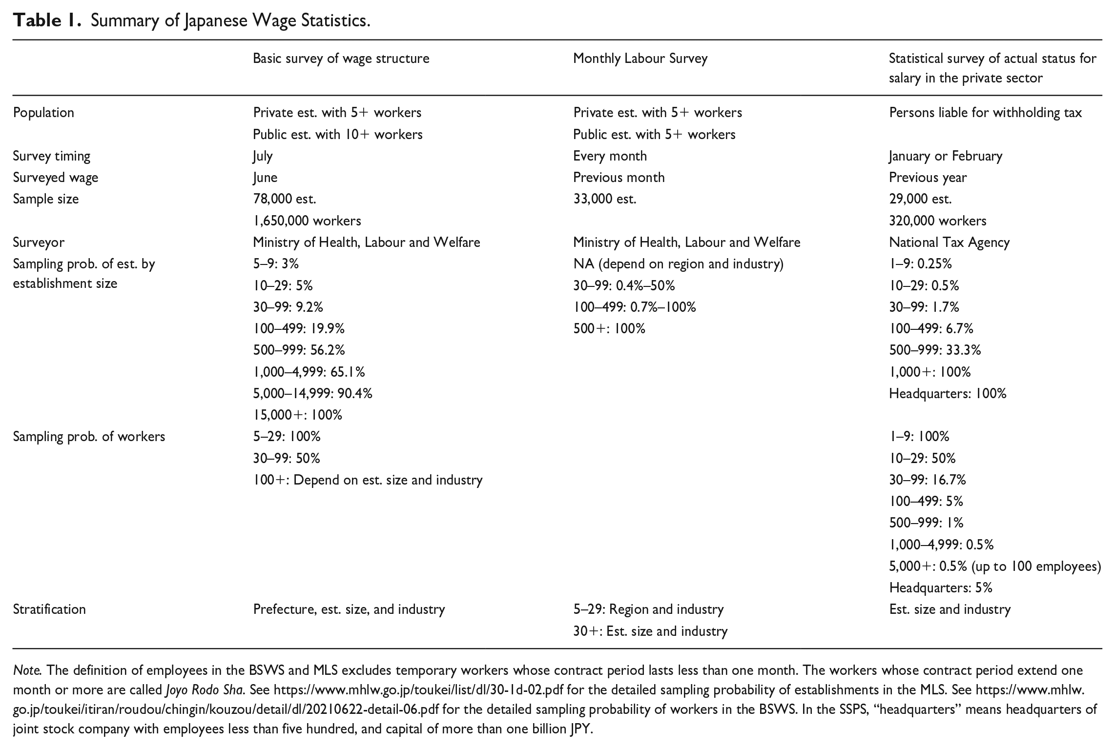
Note. The definition of employees in the BSWS and MLS excludes temporary workers whose contract period lasts less than one month. The workers whose contract period extend one month or more are called Joyo Rodo Sha. See https://www.mhlw.go.jp/toukei/list/dl/30-1d-02.pdf for the detailed sampling probability of establishments in the MLS. See https://www.mhlw.go.jp/toukei/itiran/roudou/chingin/kouzou/detail/dl/20210622-detail-06.pdf for the detailed sampling probability of workers in the BSWS. In the SSPS, “headquarters” means headquarters of joint stock company with employees less than five hundred, and capital of more than one billion JPY.

Our third data source, the MLS, is a monthly survey of establishments with five or more employees and collects the wage bill of employees at the establishment level. The rotation sampling design of the MLS with over-sampling of large establishments enables us to construct establishment-level panel data from it as well, and we match the BSWS and MLS data using the common establishment identifier assigned by the Ministry of Health, Labour and Welfare which implements both surveys and selects the establishments based on a common database. In Sections 4 and 5, we leverage this feature to validate whether the within-establishment random sampling of workers is implemented properly.

4. Establishment-Level Survey Response

Over the last half-century, Japan has experienced a continual decline in the response rate for government surveys, raising questions about potential selection bias in measures of the mean wage and mean hours worked. For instance, the response rate of the BSWS was 87% in 1982 but has declined to around 70% in recent years (Figure 1; see the Ministry of Health, Labour and Welfare (2019) for the long-term trend), which is comparable to that of establishment surveys such as the Occupational Employment and Wage Statistics survey (67% in 2021) and Economic Census (62% in 2017) in the United States and the Annual Business Survey (around 75%) in the United Kingdom, while it is lower than that of the Structural Business Statistics survey (85% in 2015) in Sweden. Although the response rates of these government-administered surveys are substantially higher than the 35.7% average response rate that Baruch and Holtom (2008) find in organizational surveys, Groves and Peytcheva (2008) note that nonresponse bias can be severe even when the response rate is high.

Figure 1.

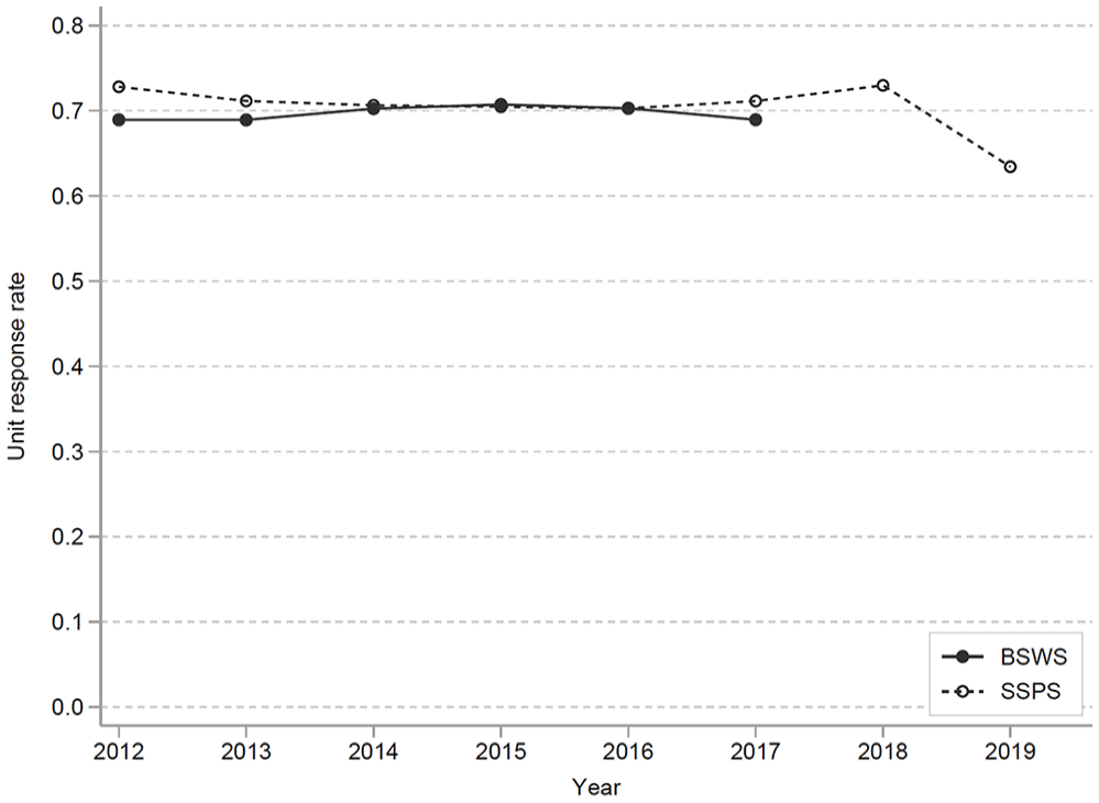
Response rates of the BSWS and SSPS.

The BSWS employs a stratified sampling design in which the strata are defined by prefecture, industry, and establishment size. As the sampling probability of establishments differs according to the characteristics of the strata, the appropriate weight for recovering the population means is the inverse of the ratio of the number of valid responses and the number of establishments in the population. The SSPS, on the other hand, stratifies establishments by size and industry, so the weight is the inverse of the ratio of the valid responses and the number of establishments within the strata.

These weights, which are designed to address the heterogeneity of response rates across strata, are appropriate for estimating the population means as long as the nonresponse behavior is ignorable within the strata. However, if the survey response probability is non-ignorable, then the published weights will not accurately estimate the population means. The source of the unit nonresponse thus plays a key role in determining whether bias correction is possible via sampling weights that incorporate the nonresponse behavior. In this light, it is important to check if the survey nonresponse is ignorable or non-ignorable by analyzing how much the survey response behavior of an establishment depends on observed and “unobserved” establishment characteristics. In this study, we approximate the unobserved characteristics by using the mean wage of the establishment that was previously observed as a proxy variable.

4.1. Relationship Between Survey Responses and Establishment Characteristics

4.1.1. The Basic Survey on Wage Structure

To characterize the survey response behavior in terms of observed characteristics of establishments, we analyze the responses by establishment size, industry, prefecture, and city size using the BSWS from 2012 to 2017, matching a list of the sampled establishments with microdata to identify the establishments with valid responses. The resulting matched data includes the indicator variable for a valid response and the variables used for stratification including the category variables of establishment size, industry, prefecture, and city size. Figure A1(a) in Appendix A shows an apparent relationship that response rate increases with establishment size. As for industry, the response rate is relatively low in wholesale and retail trade, real estate and goods leasing, accommodation and food services, lifestyle-related services and entertainment, and education and learning support services (Figure A1(b)). We also find a substantial difference in the response rate among prefectures, with that of urban areas such as Tokyo and Osaka being particularly low (Figure A1(c)).

Since the establishment characteristics of establishment size and industry are highly correlated, we disentangle the correlation through the following regression:

$$y_{itp}={x^{\prime }}_{it}\beta +{\tau }_t+{\pi }_p+u_{itp},$$

(1)

where i, t, p indicate establishment, year, and prefecture, respectively, and ${\tau }_t$ and ${\pi }_p$ are year and prefecture fixed effects. The vector of explanatory variables, ${\mathrm{x}}_{it}$ , includes dummy variables for establishment size, industry, and city population size. The dependent variable is a dummy variable for the survey response, which takes 1 if the establishment responded and 0 if not. Figure A3 shows the results of the regression analysis, which essentially confirms previous findings that establishments with fewer employees and in service industries are less likely to respond. In addition, this regression analysis also indicates that the response rate is low in the largest city category, which mainly consists of cities designated by government ordinance and core cities, which include Osaka, Nagoya, and Kyoto. As for prefectures, the response rate is lowest in Osaka, followed by Tokyo. Thus, this regression analysis suggests that the survey nonresponse is particularly severe in urban areas, which is consistent with previous studies such as Phipps and Toth (2012) and Earp et al. (2018).

Our result for the establishment size may be somewhat surprising because it is the opposite of both the empirical findings of Phipps and Toth (2012) and Earp et al. (2018) and the theoretical prediction by Tomaskovic-Devey et al. (1994) that a large establishment has difficulty responding to such a survey due to a high cost of information gathering. However, in our context, the positive correlation between response rate and establishment size is reasonable for two reasons. First, the Labor Standard Act requires each establishment to keep the wage bills of its workers, and the survey requests the establishments merely to provide a copy of these readily available wage bills for the selected workers. Thus, given this legal requirement, information processing capacity is unlikely to be a concern and, furthermore, it is reasonable to assume that a large establishment more systematically manages wage bills through electronic record-keeping than a small establishment. Second, since responding to the survey is required by the Statistics Act, large establishments are more likely to be well prepared to respond to the survey, which also supports our finding that the sampling rate is substantially higher for large establishments than small establishments.

4.1.2. The Statistical Survey of Actual Status for Salary in the Private Sector

As with the BSWS, we calculate the response rate of the SSPS for 2012 to 2019 by matching the list of sampled establishments with the microdata of the SSPS (Figure 1). Since regional information was not available, we focus on establishment size and industry in this analysis. Although the response rate is generally stable across years, we do observe a decrease from 73% in 2018 to 63% in 2019 (enumerated in 2020) due to the novel coronavirus pandemic. The reporting for 2019 occurred in early 2020, and requests and inquiries to business establishments were suspended at that time due to the declaration of a state of emergency in April 2020. A similar impact of the pandemic is also found in the CPS (Heffetz and Reeves 2021; Rothbaum and Bee 2021). In terms of establishment size, as in the BSWS, the response rate of small establishments is substantially lower (Figure A2(a)), but for establishments with one hundred or more employees, we do not observe a clear relationship between establishment size and response rate. This might be explained by two offsetting factors. First, as with the BSWS, SSPS survey response is a legal requirement and so large establishments are inclined to have high compliance. However, the SSPS is implemented via a questionnaire that is different from the readily available wage bill collected by the BSWS, and this might indeed impose higher information processing costs for large establishments. These two factors, offsetting each other, could lead to the weak correlation between response rate and establishment size observed for the SSPS. In terms of industry, the response rates for retail trade, inns/restaurants, and service are low (Figure A2(b)). In addition, the response rate for sole proprietors is significantly lower than that for corporations. These tendencies are confirmed by the regression analysis as well (Figure A4).

4.2. Serial Correlation of Survey Response Behavior

To examine whether the survey nonresponse is ignorable conditional on observed characteristics of the establishments, we investigate whether the response behavior depends on the mean of the values of previously observed characteristics of workers, including wages, at the establishment level. To implement the analysis, we construct panel data for establishments using the BSWS and SSPS. Since the sampling probability of large establishments is relatively high in both the BSWS and SSPS, it is not rare for the same establishment to be included in the sample for multiple years. Table B1 of Appendix B reports the sampling and response distributions for the BSWS from 2012 to 2017, and we see that 21% of the sampled establishments were chosen multiple times. For the SSPS from 2012 to 2019, the result was 14% (Table B2). This over-sampling allows us to construct panel data of establishments in order to analyze the dynamics of the response rates of the BSWS and the SSPS. Although this obtains panel data on only a small fraction of the sampled establishments, conditioning on the establishments sampled twice or more does not lead to a selection issue regarding survey responses because the sample establishments are randomly chosen by the survey statistician.

Regarding the response behavior of establishments conditional on the number of occasions sampled for the survey, we see that the mode of the distribution of the number of responses is equal to the number of sampled years irrespective of the number of sampled years (Tables B1 and B2). This means that while many establishments respond to the survey whether or not they have been selected for multiple years, some establishments do not respond to the survey at all even though they have been selected multiple times. This raw data suggests a strong serial correlation in the survey response behavior.

In order to shed further light on this apparent serial correlation, we estimate a linear probability model of the survey response that includes past response behavior as an explanatory variable. In particular, we estimate the following model:

$$y_{itp}={z^{\prime }}_{it}\delta +{x^{\prime }}_{it}\beta +{\tau }_t+{\pi }_p+u_{itp},$$

(2)

where $z_{it}$ is the survey response status in the previous survey(s), and the remaining part of the model is identical to Equation (1). The parameter of interest is δ, which indicates the serial correlation of the survey response behavior. In this analysis, all establishments that were sampled at least twice are included in the analysis regardless of whether they responded to the survey, while those establishments sampled only once are excluded. Column 1 of Table 2 reports the estimation results for the BSWS, and we find a substantial difference in the response rate depending upon the response to the previous survey. If an establishment responded to the previous survey, the response probability for the next survey is 0.88, but if not, the probability drops to 0.35 ( $=0.876-0.530$ ; Column 1 of Table 2). This relationship remains robust even after controlling for observed establishment characteristics.

Table 2.

Correlation Between Survey Response and Previous Survey Response(s).

Dep.Var. Survey resp.	BSWS				SSPS
	(1)	(2)	(3)	(4)	(5)	(6)	(7)	(8)
NR	−0.530 (0.004)	−0.476 (0.004)			−0.475 (0.006)	−0.461 (0.006)
NR→R			−0.205 (0.012)	−0.174 (0.011)			−0.188 (0.008)	−0.180 (0.008)
R→NR			−0.396 (0.013)	−0.360 (0.012)			−0.348 (0.009)	−0.344 (0.009)
NR→NR			−0.696 (0.010)	−0.643 (0.010)			−0.632 (0.008)	−0.622 (0.008)
Constant	0.876 (0.001)		0.920 (0.002)		0.898 (0.001)		0.920 (0.001)
Controls		X		X		X		X
Observations	107,010	107,010	29,378	29,378	70,989	70,989	48,461	48,461

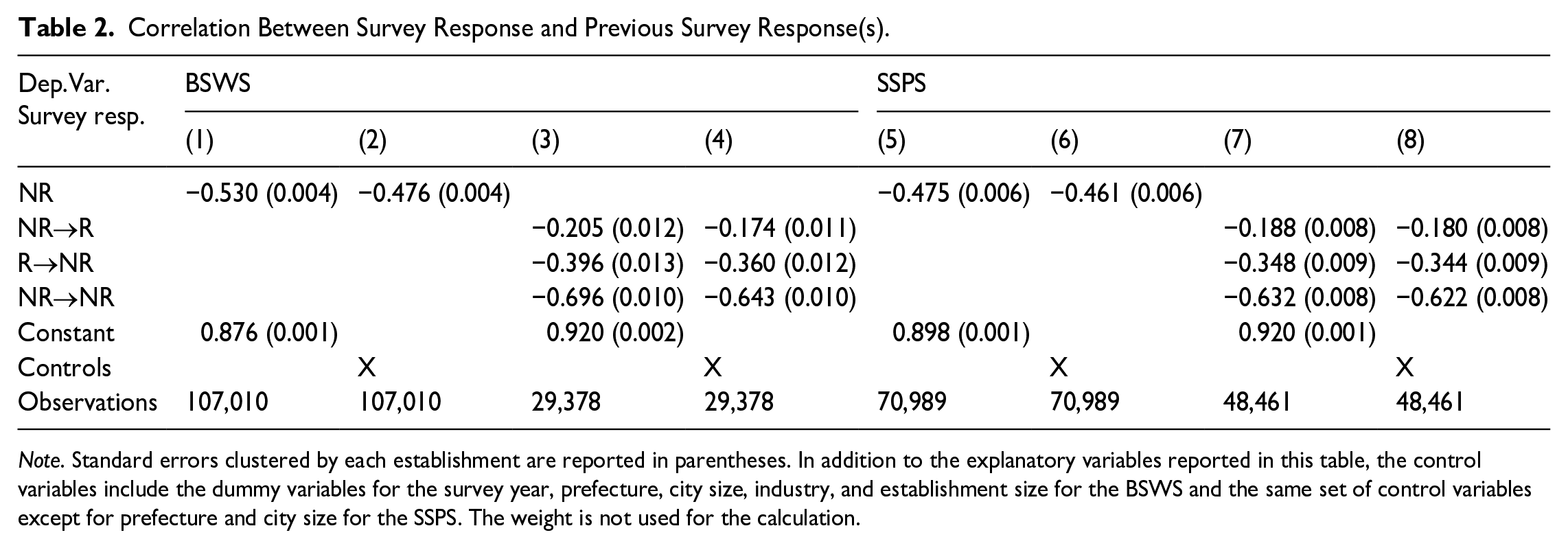
Note. Standard errors clustered by each establishment are reported in parentheses. In addition to the explanatory variables reported in this table, the control variables include the dummy variables for the survey year, prefecture, city size, industry, and establishment size for the BSWS and the same set of control variables except for prefecture and city size for the SSPS. The weight is not used for the calculation.

Columns 3 and 4 reveal that the response pattern is not explained by a simple Markov process. The variable $NR\to R$ indicates that the establishment did not respond to the survey at $t-2$ but responded at $t-1$ , where t is the time of the survey in which the establishment was sampled. Even among those establishments that responded to the previous survey, the response rate differs by 20 percentage points depending on the response status two surveys ago (Row 2 in Column 3, where the reference group is R→ R). Similarly, among those that did not respond to the previous survey, the response status two surveys ago raises the response rate by 30 percentage points (Rows 3 vs. 4 in Column 3). These results indicate that establishments with a low tendency to respond are less likely to respond this time, conditional on the response behavior of the immediate past. Columns 5 to 8 report the estimation results for the SSPS. The magnitude of the estimates is almost identical to that of the BSWS, suggesting that the underlying nonresponse structure is common across the two surveys. In sum, the survey response behavior of establishments in the current period is heavily dependent on past response behavior.

There are at least two possible explanations for this observed strong serial correlation in response behavior; namely, state dependence of response behavior and selection of establishments based on unobserved characteristics. These two explanations have very different consequences in terms of estimating the means of wages or hours worked. Regarding state dependency, such as a Markov process driven by k previous survey responses, the sample still represents the population as far as the sample selection is ignorable, conditional on the past responses. Thus, the wage statistics are unbiased as long as the Markov process is mean reverting, for this type of serial correlation only affects the standard error of the estimated wage mean. However, in the case of selection on unobserved characteristics, the wage statistics are likely to be biased. For instance, if highly productive establishments are more likely to respond, the mean wage estimated from the responding establishments would overestimate the population mean. Thus, decomposing the serial correlation into the state dependent and unobserved components is critically important.

4.3. Survey Nonresponse Based on Unobserved Characteristics

To understand the importance of survey nonresponse based on unobservables, we use lagged worker characteristics as a proxy for unobserved establishment characteristics. Specifically, we assign to each establishment-year record the mean values of workers’ wages, age, female proportion, and hours worked in the previous survey. We then regress the survey response status on those worker characteristics and the other control variables used in Equation (1):

$$y_{itp}={w^{\prime }}_{it}\delta +{{\mathrm{x}}^{\prime }}_{it}\beta +{\tau }_t+{\pi }_p+u_{itp},$$

(3)

where $w_{it}$ includes the lagged establishment characteristics, namely, the mean of workers’ wages, age, female proportion, and hours worked.

The lagged wage is of particular interest because we are mainly concerned whether survey response behavior is affected by unobserved determinants of the current wage such as the productivity of establishments. If the productivity of an establishment is constant over time, then it is reflected in past wages, so past wages serve as a good proxy for the unobserved determinant of current wages in this case. On the other hand, one may argue that productivity is time variant and past wages do not fully reflect the current economic situation. However, we show in Subsection 4.4 that even in such a case, the regression result using past wages is still informative about the relationship between the survey response and current productivity.

Table 3 reports the regression results of Equation (3). Overall, the results show a statistically significant but not economically meaningful correlation between the lagged establishment characteristics and response probability. For example, in the BSWS, a one standard deviation increase in the lagged log wage, which corresponds to 0.457 log points (Table G1), increases the response rate by 2.6 percentage points, with a 95% confidence interval of 2.2 to 2.9%. This is negligible compared to the overall response rate of 87.5% in this sample, where the response rate here is higher than that of the full sample (Column 1 of Panel A, Table G1) because this analysis sample is those establishments that responded to the survey at least once. Similarly, the estimated coefficients for workers’ age, proportion of female workers and hours worked are minute, though some of them are statistically significant. The robustness of this result is confirmed by using several other specifications, including the number of lags and its interaction with the lagged wage (Table G2). In addition, we also estimate the model using earnings instead of the hourly wage and find quantitatively similar results (Table G3).

Table 3.

Response Rate and Lagged Establishment Characteristics.

Dep.Var. Survey resp.	Panel A: BSWS
Establishment size	All	500+	100–499	30–99	5–29
	(1)	(2)	(3)	(4)	(5)
Lagged. ln(wage)	0.056 (0.004)	0.026 (0.013)	0.063 (0.007)	0.045 (0.006)	0.073 (0.006)
Lagged. Age	−0.000 (0.000)	−0.001 (0.001)	0.001 (0.000)	−0.001 (0.000)	−0.000 (0.000)
Lagged. Female	0.021 (0.006)	0.003 (0.026)	0.038 (0.014)	0.011 (0.011)	0.025 (0.010)
Lagged. ln(WorkHours)	0.065 (0.006)	0.035 (0.023)	0.085 (0.015)	0.034 (0.011)	0.075 (0.009)
Mean of Dep.Var.	0.875	0.916	0.910	0.896	0.825
Observations	91,282	8,369	21,560	27,532	33,821
Dep.Var. Survey resp.	Panel B: SSPS
Establishment size	All	500+	100–499	30–99	1–29
	(1)	(2)	(3)	(4)	(5)
Lagged. ln(earnings)	0.022 (0.003)	0.018 (0.003)	0.047 (0.011)	0.020 (0.023)	0.104 (0.025)
Lagged. Age	0.001 (0.000)	0.001 (0.000)	0.001 (0.001)	0.001 (0.002)	−0.002 (0.002)
Lagged. Female	0.021 (0.006)	0.017 (0.007)	0.027 (0.019)	0.057 (0.045)	0.056 (0.061)
Mean of Dep.Var.	0.898	0.903	0.874	0.859	0.784
Observations	59,966	53,392	4,940	975	653

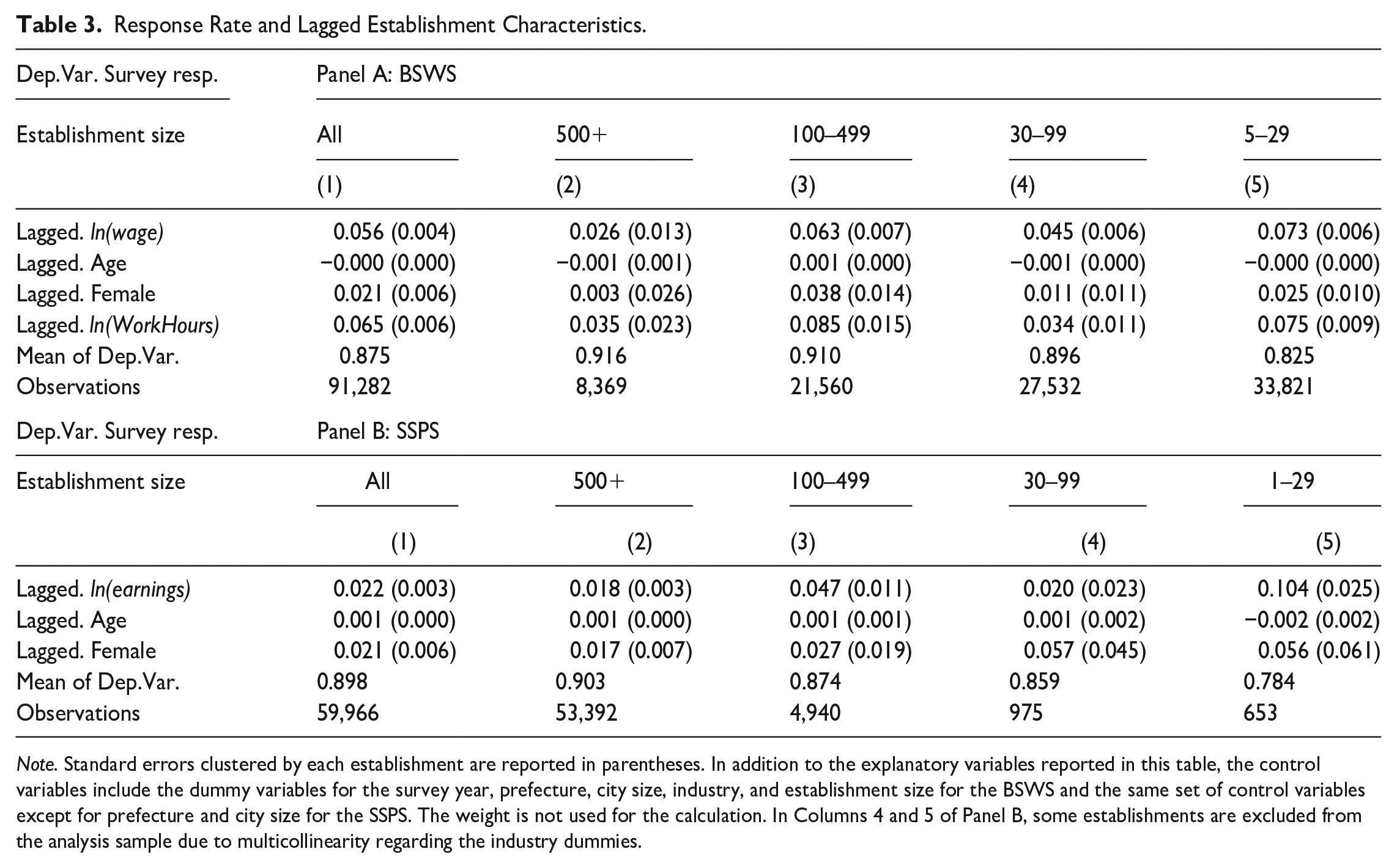
Note. Standard errors clustered by each establishment are reported in parentheses. In addition to the explanatory variables reported in this table, the control variables include the dummy variables for the survey year, prefecture, city size, industry, and establishment size for the BSWS and the same set of control variables except for prefecture and city size for the SSPS. The weight is not used for the calculation. In Columns 4 and 5 of Panel B, some establishments are excluded from the analysis sample due to multicollinearity regarding the industry dummies.

To evaluate the magnitude of unit nonresponse bias more formally, we construct the weight by estimating the Logit version of Equation (3) and then estimate mean wage and salary using an inverse probability weighting (IPW). Panel A of Table 4 shows the result of this re-weighting for the BSWS. First, the earnings and hourly wage of the panel sample tend to be higher since the sampling probability is higher for large establishments. However, comparing Columns 2 to Columns 3 to 5, we find that the mean is stable regardless of the information used to construct the IPW, though the mean decreases slightly when we control for unit nonresponse by establishment characteristics and the lagged characteristics. The results for the SSPS also show that the mean is stable irrespective of the weighting method. These results thus support our argument that unit nonresponse bias, if any, is negligible.

Table 4.

Mean Wage and Earnings With and Without Correcting for Unit Nonresponse.

Panel A: BSWS	All	Panel sample
	(1)	(2)	(3)	(4)	(5)
Total salary	32.286 [23.568]	37.994 [26.629]	37.601 [26.600]	37.343 [26.513]	37.319 [26.543]
Hourly wage	0.207 [0.163]	0.239 [0.180]	0.237 [0.180]	0.236 [0.178]	0.236 [0.179]
Weight	Built-in	Built-in	IPW	IPW	IPW
Year			X	X	X
Industry			X	X	X
Establishment size			X	X	X
Prefecture			X	X	X
City size			X	X	X
Lagged wage				X	X
Other lagged characteristics					X
Observations	7,272,729	2,207,368	2,207,368	2,207,368	2,207,368
Panel B: SSPS	All	Panel sample
	(1)	(2)	(3)	(4)	(5)
Total salary	31.565 [31.263]	36.346 [34.422]	36.712 [34.655]	36.532 [34.574]	36.535 [34.579]
Weight	Built-in	Built-in	IPW	IPW	IPW
Year			X	X	X
Industry			X	X	X
Establishment size			X	X	X
Prefecture
City size
Lagged wage				X	X
Other lagged characteristics					X
Observations	2,402,129	1,317,657	1,317,657	1,317,657	1,317,657

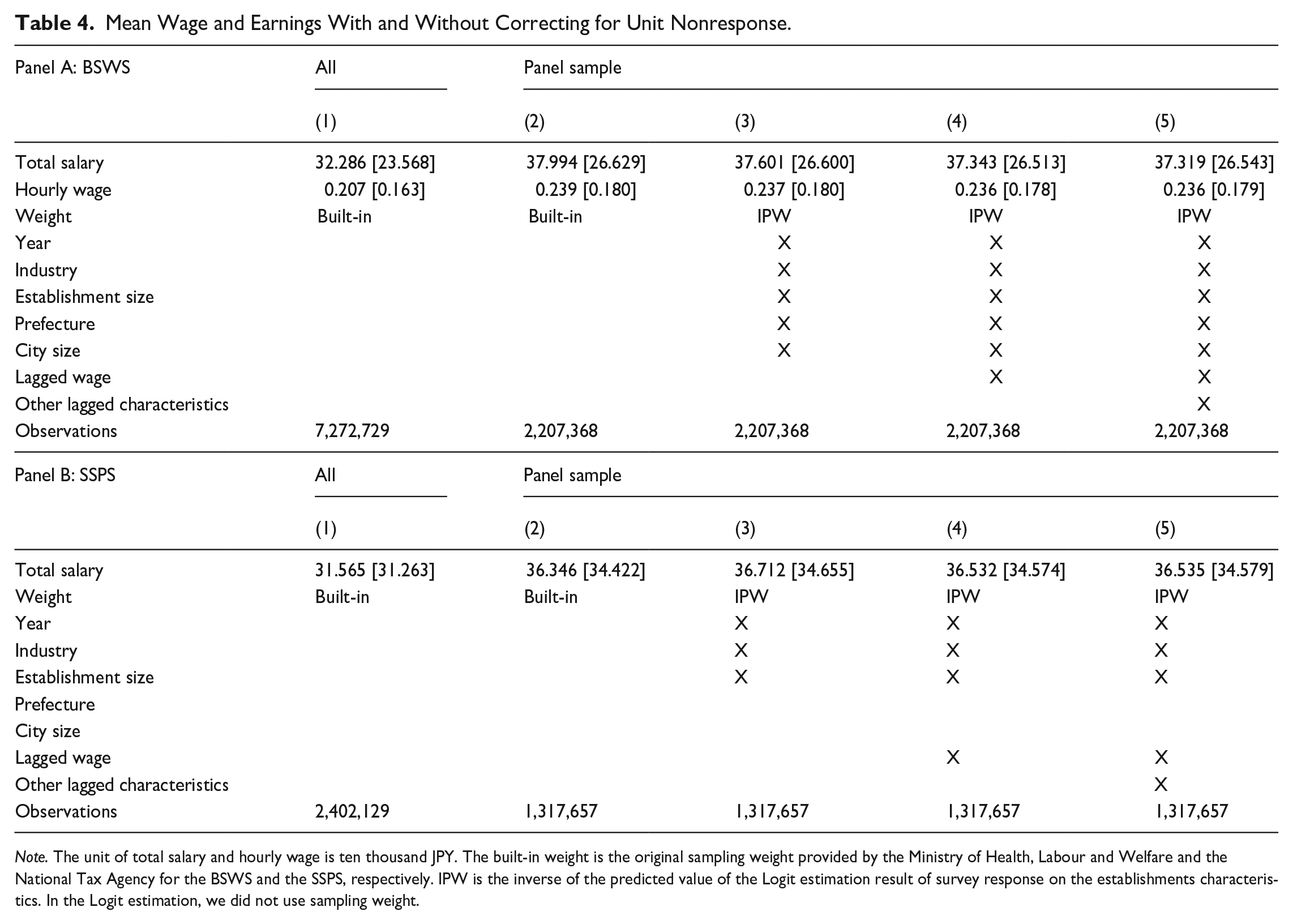
Note. The unit of total salary and hourly wage is ten thousand JPY. The built-in weight is the original sampling weight provided by the Ministry of Health, Labour and Welfare and the National Tax Agency for the BSWS and the SSPS, respectively. IPW is the inverse of the predicted value of the Logit estimation result of survey response on the establishments characteristics. In the Logit estimation, we did not use sampling weight.

Since the response rate varies substantially by establishment size, it is of particular interest whether the unit nonresponse on unobservables is substantial among small establishments. However, the results of the subsample analysis, reported in Columns 2 to 5 of Table 3, show little systematic heterogeneity. If anything, the selection in terms of the lagged hourly wage is relatively distinct for the smallest establishment group, but the size of its estimate is still moderate. In fact, the estimation results show that a 1 SD increase (0.457 log points) in the lagged mean wage increases the unit response rate only by 3.3 percentage points. Panel B of Table 3 reports the estimation results of the same analysis using SSPS 2012 to 2019, for which we use annual earnings instead of hourly wages because work hours are not surveyed in the SSPS. The SSPS estimates are economically insignificant as well.

4.4. Unit Nonresponse Based on the Current Wage

4.4.1. Unit Nonresponse by Wage Level

The analysis in the previous section correlates response behavior with the past wage, but a valid concern is that the survey response may be determined not by the past wage but by the current wage. If this is true, how can we interpret the results using the past wage? Since the fundamental problem in analyzing nonresponse bias is that we cannot observe the variable of interest in the survey data, it is difficult to draw conclusions on nonresponse bias by unobservables without an auxiliary data set such as administrative records. However, if we assume that wages are serially correlated, this allows us to link the current wage and the past wage and thereby to analyze nonresponse bias based on the current wage.

While there are many potential unobserved factors contributing to survey nonresponse, we focus on the current wage as a source of nonresponse in this analysis. A main reason for this is that the relationship between the survey response and the wage is a summary statistic of the nonresponse bias in terms of the wage distribution. In fact, the probability density function of the wage is written as $f(w)=\mathrm{Pr}(d=1)f(w|d=1)+\mathrm{Pr}(d=0)f(w|d=0)$ , where d is an indicator for the unit-response, and by Bayes’ theorem, we have $f(w|d=0)=\frac{\mathrm{Pr}(d=0|w)f(w)}{\mathrm{Pr}(d=0)}$ . Since we have two equations and two unknowns, $f(w)$ and $f(w|d=0)$ , solving this system of equations, we obtain

$$f(w|d=0)=\frac{\mathrm{Pr}(d=1)/\mathrm{Pr}(d=1|w)}{\mathrm{Pr}(d=0)/\mathrm{Pr}(d=0|w)}f(w|d=1).$$

(4)

Therefore, as long as it is only the wage distribution that is of interest, considering the survey nonresponse caused by the wage is sufficient. As mentioned above, the fundamental problem is that we cannot observe either $f(w|d=0)$ or $\mathrm{Pr}(d=0|w)$ . However, if we assume a time-series structure on the wage, this assumption, combined with the panel structure of the data, provides a useful source of identification.

To formalize this, let $d_{it}$ and $w_{it}$ be unit response and log wage for establishment i and year t. If the unit response is determined by the level of the wages of the establishment, the unit response behavior is conceptually specified as

$$d_{it}={\beta }_0+{\beta }_1{w}_{it}+u_{it},$$

(5)

where ${\beta }_1\ne 0$ implies the presence of non-ignorable nonresponse. A main challenge in estimating Equation (5) is that $w_{it}$ is unobserved for non-respondents; that is, if $d_{it}=0$ . To overcome this issue, we assume that the establishment wage follows an AR(1) process:

$$w_{it}=\rho w_{it-1}+{\eta }_{it},$$

(6)

where ${\eta }_{it}$ is drawn from an independent and identically distributed. We note that this AR(1) assumption is common in the income process literature (e.g., Guvenen 2009), and if an individual wage follows an AR(1) process, then the establishment-average wage also follows an AR(1) process. With this assumption, the unit response model (5) is rewritten as

$$d_{it}={\beta }_0+{\tilde{\beta }}_1^{(1)}{w}_{it-1}+{\tilde{u}}_{it}^{(1)},$$

(7)

where ${\tilde{\beta }}_1^{(1)}={\beta }_1\rho$ and ${\tilde{u}}_{it}^{(1)}={\beta }_1{\eta }_{it}+u_{it}$ . Importantly, the OLS estimate of equation (5) is confounded when ${\eta }_{it}$ is correlated with $u_{it}$ , but this correlation does not affect the consistency of the OLS estimate of Equation (7) as long as ${\eta }_{it-1}$ is orthogonal to $u_{it}$ . Hence, ${\tilde{\beta }}_1^{(1)}$ is consistently estimated even if ${\eta }_{it}$ is correlated with $u_{it}$ . Thus, the key assumption is that ${\eta }_{it-1}$ and ${\eta }_{it}$ are not correlated, so if the AR(1) process properly captures the data generating process, the absence of serial correlation of ${\eta }_{it}$ is assured. Furthermore, for $s=1,2,\dots$ , the model (5) is rewritten as

$$d_{it}={\beta }_0+{\tilde{\beta }}_1^{(s)}{w}_{it-s}+{\tilde{u}}_{it}^{(s)},$$

(8)

where ${\tilde{\beta }}_1^{(s)}={\beta }_1{\rho }^s$ and ${\tilde{u}}_{it}^{(s)}=u_{it}+{\beta }_1{\sum }_{k=0}^{s-1}{\rho }^k{\eta }_{it-k}$ , and ${\tilde{\beta }}_1^{(s)}$ is consistently estimated by OLS. Therefore, it follows that the persistency parameter ρ of the AR(1) process and ${\beta }_1$ , the parameter of interest, are estimated by

$$\widehat{\rho }=\frac{{\widehat{\tilde{\beta }}}_1^{(s+1)}}{{\widehat{\tilde{\beta }}}_1^{(s)}}and{\widehat{\beta }}_1^{level}=\frac{{\widehat{\tilde{\beta }}}_1^{(s)}}{{\widehat{\rho }}^s}$$

(9)

Furthermore, in the particular case of a random walk (i.e., $\rho =1$ ), Equation (9) shows that ${\widehat{\beta }}_1^{level}={\widehat{\tilde{\beta }}}_1^{(s)}$ , and thus ${\beta }_1$ can be directly estimated as a coefficient on the lagged wage.

4.4.2. Unit Nonresponse by Wage Growth

Alternatively, one may argue that time-variant unobserved characteristics can affect the current wages, and that this is better captured by changes in the wage than the level of the wage. In this case, the unit response could be determined by the growth of the establishment wage, so that

$$d_{it}={\beta }_0+{\beta }_1\Delta w_{it}+u_{it}.$$

(10)

Then, the unit response model (10) is rewritten as

$$d_{it}={\beta }_0+{\stackrel{··}{\beta }}_1^{(s)}{w}_{it-s}+{\stackrel{··}{u}}_{it}^{(s)},$$

(11)

where ${\stackrel{··}{\beta }}_1^{(s)}={\beta }_1(\rho -1){\rho }^{s-1}$ and ${\stackrel{··}{u}}_{it}^{(s)}=u_{it}+{\beta }_1{\sum }_{k=0}^{s-1}{(\rho -1)}^k{\eta }_{it-k}$ . Again, ${\stackrel{··}{\beta }}_1^{(s)}$ is consistently estimated by OLS as long as $u_{it}$ is orthogonal to ${\eta }_{is}$ for $s<t$ , and thus,

$$\widehat{\rho }=\frac{\cdot \widehat{\beta }{\cdot }_1^{(s+1)}}{{\widehat{\stackrel{··}{\beta }}}_1^{(s)}}\mathrm{and}{\widehat{\beta }}_1^{growth}=\frac{{\widehat{\stackrel{··}{\beta }}}_1^{(s)}}{\left(\widehat{\rho }-1\right){\widehat{\rho }}^{s-1}}$$

(12)

for $\rho \ne 1$ . In the special case of a random walk, we have ${\stackrel{··}{\beta }}_1^{(s)}={\beta }_1(\rho -1){\rho }^{s-1}=0$ , suggesting no correlation between the unit response and the past wage.

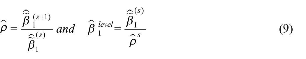
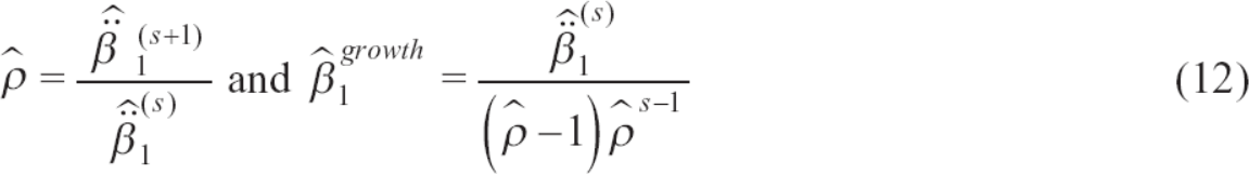
The above argument has three implications. First, the persistence, ρ, of AR(1) is consistently estimated as a fraction of the OLS estimates of the unit response on lagged wages as shown in Equations (9) and (12), irrespective of the model specification (5) or (10). Second, the model is over-identified with three-period or longer panel data, and we can test if $\widehat{\rho }$ does not depend on the number of lags s under the correct specification, though it is estimated as a fraction of the coefficients on $(s+1)$ -th and $s-\mathrm{th}$ lagged wages. Third, in the case of a random walk, ${\stackrel{··}{\beta }}_1^{(s)}=0$ , so we can reject model (10) in which the unit response is determined by wage growth, if the estimated coefficient on the lagged wage is statistically significant.

Table 5 shows the estimation results. In both surveys, the coefficients on lagged wage and earnings are statistically significant regardless of the number of lags s, though the estimate becomes imprecise for large s due to the small sample size. The second row reports the estimated values for ρ and we cannot reject the random walk (i.e., $H_0$ : $\rho =1$ ). Therefore, combining these two results, our empirical evidence does not support the unit response model in which the response behavior depends on wage growth. Furthermore, our estimates for ${\beta }_1^{level}$ tend to be stable over the number of lags s, though the estimates are imprecise for $s\ge 4$ again due to the smaller sample size, whereas the estimates for ${\beta }_1^{growth}$ are unstable and imprecise regardless of s, which also supports the unit response model based on the current wage level rather than wage growth. In addition, equation (9) shows that when the wage process is close to a random walk, the magnitude of ${\widehat{\beta }}_1^{level}$ is comparable to the magnitude of the estimated coefficient on lagged wage and earnings. Thus, we can regard the coefficient of the lagged wage as a good approximation of the coefficient of the current wage in this case. This result partly justifies our specification (3), which simply includes the lagged wage observed most recently. Finally, we see that the estimates for ρ in the fifth row are not statistically different from each other which is also, at minimum, consistent with the implication from our model.

Table 5.

Unit Nonresponse Based on the Current Wage.

Panel A: BSWS	$s=1$	$s=2$	$s=3$	$s=4$	$s=5$
Dep.Var. Unit response	(1)	(2)	(3)	(4)	(5)
$\ln wag{e}_{it-s}$	0.048 (0.004)	0.058 (0.006)	0.064 (0.007)	0.072 (0.009)	0.074 (0.015)
${\widehat{\rho }}^{(s)}={\widehat{\beta }}^{(s+1)}/{\widehat{\beta }}^{(s+1)}$	1.205 (0.135)	1.108 (0.133)	1.120 (0.153)	1.037 (0.219)
${\widehat{\beta }}_1^{level}$	0.040 (0.007)	0.047 (0.014)	0.045 (0.021)	0.062 (0.056)
${\widehat{\beta }}_1^{growth}$	0.233 (0.165)	0.480 (0.672)	0.422 (0.675)	1.747 (11.617)
p-Value $\left(H_0:{\rho }^{(s)}={\rho }^{(s^{\prime })}\right)$	.913
Observations	55,578	31,794	23,952	14,404	5,391
Panel B: SSPS	$s=1$	$s=2$	$s=3$	$s=4$	$s=5$	$s=6$	$s=7$
Dep.Var. Unit response	(1)	(2)	(3)	(4)	(5)	(6)	(7)
$\ln earning{s}_{it-s}$	0.015 (0.003)	0.019 (0.003)	0.022 (0.004)	0.023 (0.005)	0.018 (0.006)	0.015 (0.007)	0.019 (0.010)
${\widehat{\rho }}^{(s)}={\widehat{\beta }}^{(s+1)}/{\widehat{\beta }}^{(s+1)}$	1.314 (0.200)	1.147 (0.157)	1.031 (0.162)	0.798 (0.172)	0.842 (0.270)	1.209 (0.523)
${\widehat{\beta }}_1^{level}$	0.011 (0.003)	0.015 (0.006)	0.020 (0.011)	0.057 (0.050)	0.043 (0.071)	0.005 (0.013)
${\widehat{\beta }}_1^{growth}$	0.043 (0.071)	0.005 (0.013)	0.047 (0.035)	0.115 (0.147)	0.670 (3.719)	−0.224 (0.068)
p-Value $\left(H_0:{\rho }^{(s)}={\rho }^{(s^{\prime })}\right)$	.296
Observations	50,219	40,944	32,641	24,848	17,911	11,410	5,513

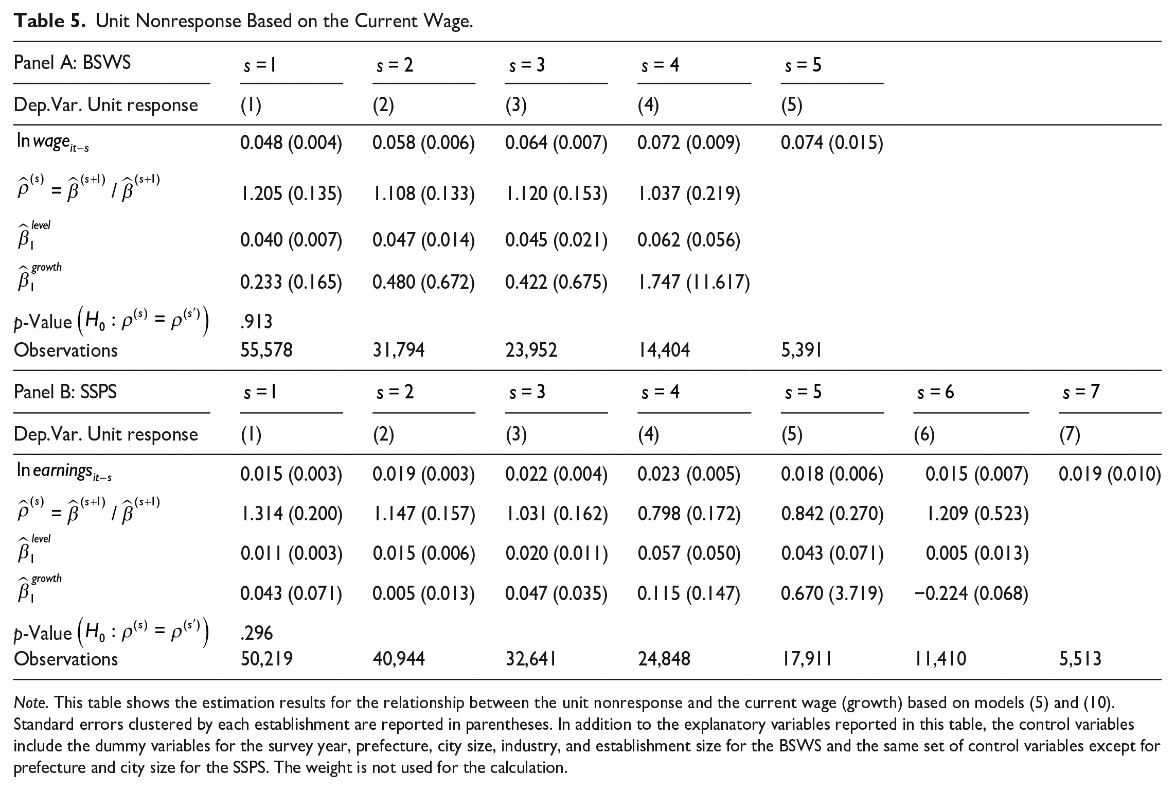
Note. This table shows the estimation results for the relationship between the unit nonresponse and the current wage (growth) based on models (5) and (10). Standard errors clustered by each establishment are reported in parentheses. In addition to the explanatory variables reported in this table, the control variables include the dummy variables for the survey year, prefecture, city size, industry, and establishment size for the BSWS and the same set of control variables except for prefecture and city size for the SSPS. The weight is not used for the calculation.

4.5. Unit Nonresponse Bias from Establishments That Never Responded to the Survey: Difficult-to-Reach Establishments

One caveat to the analysis in the previous section is that it does not consider nonresponse bias based on unobserved characteristics among establishments that never responded to the survey despite being sampled at least twice. Although the proportion of those establishments is relatively low, at 12% in the BSWS and 7% in the SSPS, those establishments could be a substantially selective group despite their relatively small representation, so the resulting bias may be non-negligible.

To evaluate the magnitude of nonresponse bias caused by these establishments, we conduct an analysis based on the continuum of resistance model, which assumes that non-respondents are well-approximated by respondents who were difficult to contact. The idea of using such difficult-to-contact information was originally proposed by Politz and Simmons (1949) and developed by Potthoff et al. (1993), and while this approach is widely recognized in the statistics and survey methodology literatures, its application in the economics literature is relatively limited (Biemer et al. 2013; Heffetz and Rabin 2013; Heffetz and Reeves 2019). In household surveys, difficult-to-reach respondents are usually defined as those who required many callbacks to participate. However, since we do not have data on the number of callbacks, we instead define difficult-to-reach establishments as those that responded to the survey only once even though they were sampled several times. Thus, this analysis assumes that the wage distribution of establishments that never responded to the survey is approximated by the wage distribution of these difficult-to-reach establishments.

In particular, we estimate the following equation:

$$\ln wag{e}_{ijtp}=\sum _{s=1}^{S-1}{\gamma }_s^{S}1\left\{\mathrm{\#Responses}=s\right\}+x_{it}^{\prime }{\mathrm{\beta }}^S+{\tau }_t^S+{\pi }_p^S+u_{itp},$$

(13)

where i, j, t, and p indicate the establishment, worker, year, and prefecture, and $x_{it}$ includes the same set of establishment characteristics as before. We denote the number of sampled years by S, so the reference group in Equation (13) is easy-to-reach establishments, or the establishments that always responded when sampled. Since the interpretation of the coefficient of interest, ${\gamma }_s^S$ , depends on the number of years sampled by the survey, we estimate this equation separately by the number of sampled years. We note that the literature mainly uses cross-sectional data for this analysis and the difficult-to-reach respondents are used to approximate all non-respondents. However, we have panel data and so difficulty to reach is defined by the number of responses in past surveys. Therefore, our target for approximation is those establishments that never responded to the survey as opposed to all non-respondents.

Table 6 shows the estimation results for Equation (13). For the BSWS, the hourly wage of difficult-to-reach establishments tends to be lower by 5 to 16% than easy-to-reach establishments. The results for the SSPS are similar to the BSWS for establishments that were sampled five times or less, but for difficult-to-reach establishments sampled more than five times, earnings are substantially lower. However, we point out that these establishments are quite rare, as the share of difficult-to-reach establishments is 1.2, 0.4, and 0.2% for those sampled six, seven, and eight times in the SSPS. Conditional on establishments sampled at least twice, the employment share of establishments that never responded to the survey is 6.3% for the BSWS and 4.6% for the SSPS. Assuming that their wage is, on average, lower by 16% for the BSWS and 51% $(=\exp (-0.712)-1)$ for the SSPS than the establish-ments that responded to the survey, the resulting size of the bias is 1.0 % $\left(=100\times \left(1-\frac{0.937\times w+0.063\times (1-0.16)w}{w}\right)\right)$ for the BSWS and 2.3% for the SSPS. Therefore, this analysis suggests that, assuming that difficult-to-reach establishments serve as a good approximation of those that never responded, the bias in the mean wage estimate is relatively small. However, this does not assure a negligible bias over the entire wage distribution, and one needs to be particularly careful when the left tail of the wage distribution is concerned.

Table 6.

Mean Wage and Earnings by Difficulty to Reach.

Panel A: BSWS	#Sample = 2		#Sample = 3		#Sample = 4		#Sample = 5		#Sample = 6
Dep.Var ln wage	Diff.	Share (%)	Diff.	Share (%)	Diff.	Share (%)	Diff.	Share (%)	Diff.	Share (%)
	(1)	(2)	(3)	(4)	(5)	(6)	(7)	(8)	(9)	(10)
#Response = 1	−0.056 (0.015)	11.1	−0.130 (0.037)	2.7	−0.157 (0.065)	0.8	−0.129 (0.087)	0.4	0.004 (0.172)	0.4
#Response = 2	0.000	88.9	−0.072 (0.019)	12.9	−0.044 (0.039)	3.2	−0.161 (0.067)	0.7	0.208 (0.075)	0.6
#Response = 3			0.000	84.4	−0.007 (0.027)	12.1	0.040 (0.046)	2.4	−0.030 (0.083)	2.3
#Response = 4					0.000	83.8	0.015 (0.035)	10.0	−0.275 (0.079)	1.2
#Response = 5							0.000	86.4	0.023 (0.077)	11.5
#Response = 6									0.000	84.0
Observations	2,080,242		838,630		459,934		437,389		51,044
Panel B: SSPS	#Sample = 2		#Sample = 3		#Sample = 4		#Sample = 5		#Sample = 6		#Sample = 7		#Sample = 8
Dep.Var. ln earnings	Diff.	Share (%)	Diff.	Share (%)	Diff.	Share (%)	Diff.	Share (%)	Diff.	Share (%)	Diff.	Share (%)	Diff.	Share (%)
	(1)	(2)	(3)	(4)	(5)	(6)	(7)	(8)	(9)	(10)	(!1)	(12)	(13)	(14)
#Response = 1	−0.089 (0.023)	13.6	−0.182 (0.082)	3.9	0.019 (0.093)	1.8	−0.138 (0.113)	1.4	−0.687 (0.124)	1.2	−0.478 (0.209)	0.4	−0.712 (0.377)	0.2
#Response = 2	0.000	86.4	−0.019 (0.040)	18.3	−0.087 (0.071)	5.8	−0.193 (0.107)	3.7	−0.051 (0.166)	1.8	0.175 (0.256)	0.6	−0.203 (0.128)	0.6
#Response = 3			0.000	77.7	0.057 (0.046)	21.0	−0.214 (0.147)	7.4	−0.073 (0.119)	5.1	−0.269 (0.119)	1.8	−0.301 (0.261)	1.3
#Response = 4					0.000	71.4	−0.181 (0.081)	22.8	0.032 (0.123)	7.6	−0.396 (0.151)	2.9	−0.206 (0.077)	2.3
#Response = 5							0.000	64.7	0.069 (0.092)	26.1	0.210 (0.138)	11.7	−0.171 (0.074)	2.9
#Response = 6									0.000	58.2	−0.298 (0.111)	18.3	0.006 (0.082)	7.9
#Response = 7											0.000	64.3	−0.095 (0.051)	17.4
#Response = 8													0.000	67.4
Observations	181,938		116,663		102,961		93,264		91,618		128,880		1,051,513

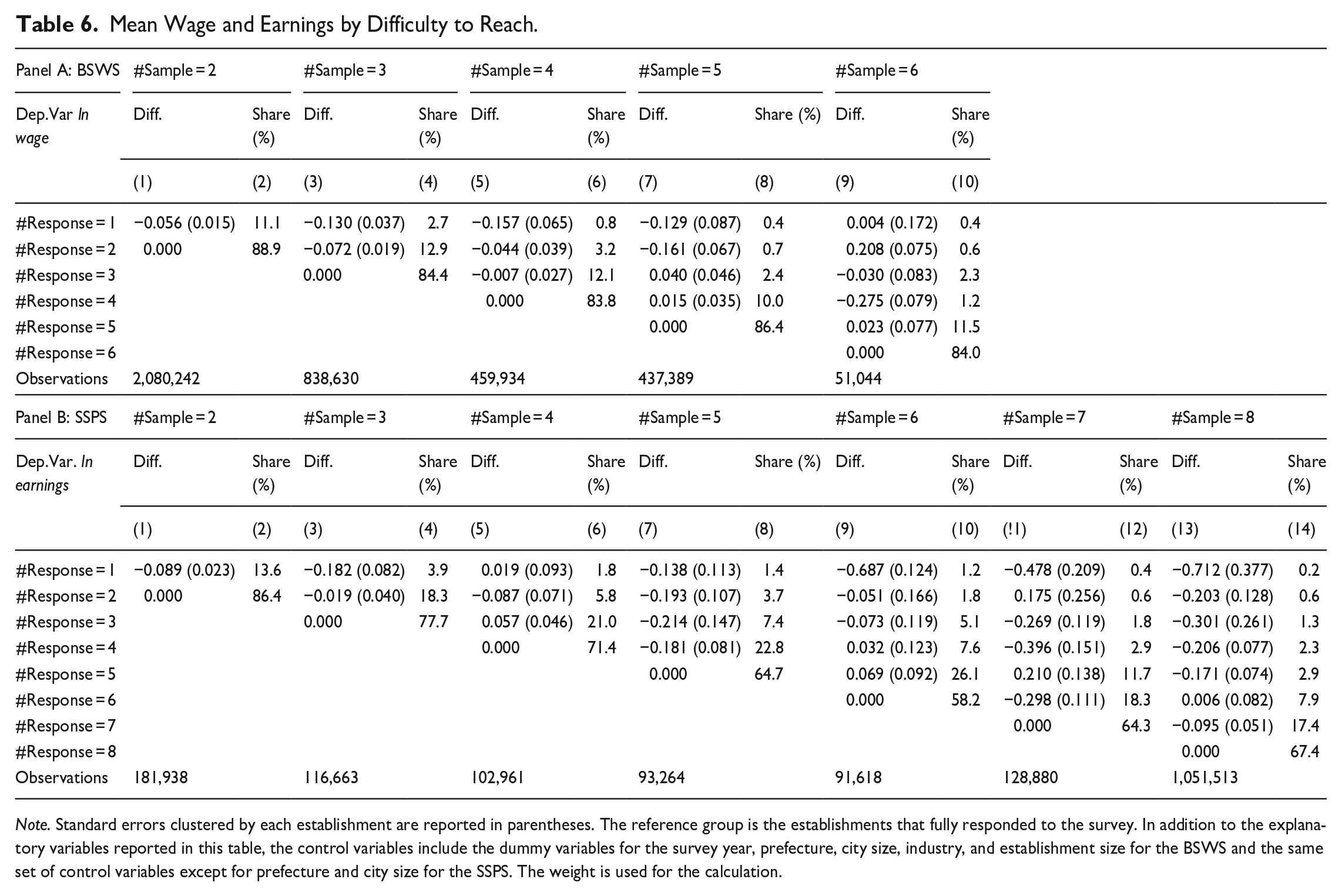
Note. Standard errors clustered by each establishment are reported in parentheses. The reference group is the establishments that fully responded to the survey. In addition to the explanatory variables reported in this table, the control variables include the dummy variables for the survey year, prefecture, city size, industry, and establishment size for the BSWS and the same set of control variables except for prefecture and city size for the SSPS. The weight is used for the calculation.

As a remark, we note that the assumption that non-respondents are approximated by difficult-to-reach respondents, though intuitive and appealing, is not always justified depending on the survey context. For example, Lin and Schaeffer (1995) evaluate the validity of this assumption by using data from the telephone survey for child support awards and payments in Wisconsin matched with the Court Record Database and find some evidence inconsistent with this assumption. However, that survey context is quite different from the large-scale government surveys analyzed in this article, as pointed out by Heffetz and Reeves (2019). In a context more similar to ours, Kreuter et al. (2010) link the German “Labor Market and Social Security” panel study commissioned by the Institute for Employment Research (IAB) to administrative data, and find evidence consistent with the continuum of resistance model. Nonetheless, to at least partially address the potential concern posed by Lin and Schaeffer (1995), in Section 7 we supplement our main analysis with a case study that uses the administrative tax records of one large city.

Overall, our empirical evidence suggests that survey nonresponse is partly driven by unobserved establishment characteristics including productivity, but the resulting bias seems to be negligible as long as it is the mean or median that is of interest. In fact, our analysis using the past wage shows that the correlation between the survey response and the establishment current or past wage is economically not meaningful. Furthermore, the imputation of missing wages by using the wages of difficult-to-reach establishments finds the size of the bias to be at most 2.3%. Together, this empirical evidence argues in favor of state dependency rather than nonresponse on unobservables as the reason for the strong serial correlation of the survey response discussed in Subsection 4.2.

4.6. Supplementary Establishments in the Basic Survey on Wage Structure

In the BSWS, when a selected establishment does not respond to the survey, an additional establishment is sampled from a pool of supplementary establishments to achieve the survey’s predetermined precision for the mean estimate. We find that about 6% of the establishments that responded to the survey did not appear in the original list of sampled establishments, so these were presumably selected from the supplementary establishment pool. As supplementary establishments are typically smaller (see Appendix D for more detailed characteristics), if only establishments that are likely to respond to the survey are used as a supplementary sample, the establishment distribution in the sample would differ from that of the population. This type of substitution does not help to mitigate nonresponse bias based on unobserved characteristics in general, and if the substitution pool tends to have more establishments with high wages, the bias could even be amplified. However, if the unit-response structure of the supplementary establishments is the same as the original pool of establishments, the substitution improves precision without changing the bias. Therefore, since whether the substitution improves or worsens data quality is an empirical question, in this subsection, we have addressed this situation by comparing the wage payments of establishments listed and not listed in the supplementary establishment pool.

Although any difference in the mean wages of establishments on the original survey list and the supplementary list would bias the estimate of mean wages, if the difference is negligible within a prefecture-firm size-industry cell, using a proper weighting procedure would correct the potential bias. To examine if this is the case, we regress the individual workers’ wage on the indicator of the supplementary establishment, along with the survey year, establishment size, industry, and prefecture fixed effects. Table 7 reports the estimation results, and Column 1 shows that the average wage of supplementary establishments is about 13% lower than that of listed establishments when we do not condition on industry, establishment size, and prefecture fixed effects. However, this difference is reduced to only 1.1% and becomes statistically insignificant after conditioning on these fixed effects, as reported in Column 4. Note that, given the sample size, this lack of significance is not due to an imprecise estimate, and indeed the 95% confidence interval ranges from –2.8 to 0.7%, suggesting an economically small difference. This result implies that even if supplementary establishments are used, the resulting bias would not be serious after appropriately adjusting the distribution for the observed establishment characteristics. Therefore, in our particular case, the sampling with substitution increases the sample size and thus improves the precision of the resulting statistics without affecting the size of the bias.

Table 7.

Regression Analysis: Listed Versus Unlisted Establishments (BSWS 2012–2017).

Dep.Var. ln(earnings)	(1)	(2)	(3)	(4)
Supplementary	−0.128 (0.011)	−0.042 (0.009)	−0.014 (0.008)	−0.011 (0.009)
Year	X	X	X	X
Industry		X	X	X
Establishment size			X	X
Prefecture				X
Observations	7,833,796	7,833,796	7,833,796	7,833,796

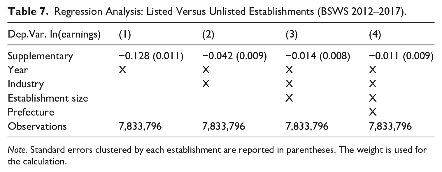
Note. Standard errors clustered by each establishment are reported in parentheses. The weight is used for the calculation.

5. Sampling of Workers Within Establishments

A peculiar feature of the BSWS and SSPS is that both surveys delegate the sampling of workers within the establishments to the survey respondents. Although both surveys provide instructions on how to conduct the random sampling, it is not inconceivable that an inexpert respondent might implement the random sampling inappropriately. In this section, we investigate whether the random sampling was conducted properly by comparing the mean wages calculated based on establishment-level aggregate data and individual worker-level data. If the random sampling was properly implemented, these two statistics should be equal.

5.1. The Basic Survey on Wage Structure

We first examine the procedure for the random sampling of workers for the BSWS. Since the BSWS establishment survey does not ask for the aggregate wage bill and total hours worked, we cannot directly calculate average wages based on establishment-level aggregate statistics. To overcome this data limitation, we first match the establishment in the BSWS with the same establishment in the Monthly Labour Survey (MLS). As explained in the data section above, the MLS is a monthly establishment survey asking about the monthly aggregate wage bill as well as aggregate hours worked. Since the BSWS and the MLS can be matched at the establishment level by using the common establishment identifier, we are able to check whether the average wage payment per worker calculated from each of these two surveys is consistent. The MLS data includes the total number of full-time workers, aggregate actual working hours, and aggregate paid salaries, and from this information, we calculate the hours worked per worker by dividing the total number of hours worked by the number of permanent workers at each establishment. Similarly, we calculate the salary per worker by dividing the total salaries paid by the number of permanent workers. If the workers selected individually in the BSWS were randomly sampled within an establishment, then the hours worked and salary per full-time worker calculated from the individual surveys should, on average, match those calculated from the MLS. Therefore, by calculating the difference between the values obtained from the BSWS and the MLS, it is possible to infer the randomness of the sampling of workers and, if not random, which type of workers are more likely to be included in the sample.

The process of constructing the analysis sample is shown in Table 8. Column 1 reports the statistics of all observations in the BSWS. We then first restrict our sample to establishments with five hundred or more workers from the BSWS 2016 to 2017 (Column 2) because the MLS, at least in principle (see below), does not sample but instead surveys all establishments with five hundred or more employees, but this does not apply to smaller establishments, which are sampled.

Table 8.

Sampling of Workers Within an Establishment: BSWS Versus MLS.

	BSWS			MLS	Diff.
	All	500+	Matched		(3)−(4)	(3)−(2)
	(1)	(2)	(3)	(4)	(5)	(6)
Number of employees	33.94 [109.80]	962.34 [1,101.64]	1,147.16 [1,209.31]	1,153.22 [1,167.76]	−6.06 (16.65)	184.82 (21.19)
Work days	20.00 [5.25]	20.05 [3.58]	20.13 [3.43]	19.59 [2.22]	0.54 (0.06)	0.08 (0.04)
Predetermined work hours	140.14 [50.27]	149.46 [33.02]	151.10 [31.50]	147.26 [20.52]	3.84 (0.48)	1.64 (0.40)
Overtime hours	7.55 [15.57]	12.88 [17.95]	14.66 [18.34]	15.57 [9.81]	−0.91 (0.18)	1.78 (0.18)
Total work hours	147.70 [56.46]	162.34 [40.56]	165.76 [39.57]	162.83 [25.05]	2.93 (0.53)	3.42 (0.48)
Salary paid on a fixed basis	22.89 [14.74]	36.65 [21.17]	36.84 [19.60]	36.63 [10.26]	0.21 (0.13)	0.19 (0.23)
Bonus	3.57 [5.91]	9.93 [10.74]	10.80 [9.94]	11.41 [6.24]	−0.61 (0.07)	0.87 (0.14)
Total salary	26.47 [18.84]	46.58 [29.16]	47.64 [27.36]	48.04 [15.43]	−0.40 (0.18)	1.06 (0.34)
Observations	114,410	5,037	2,193

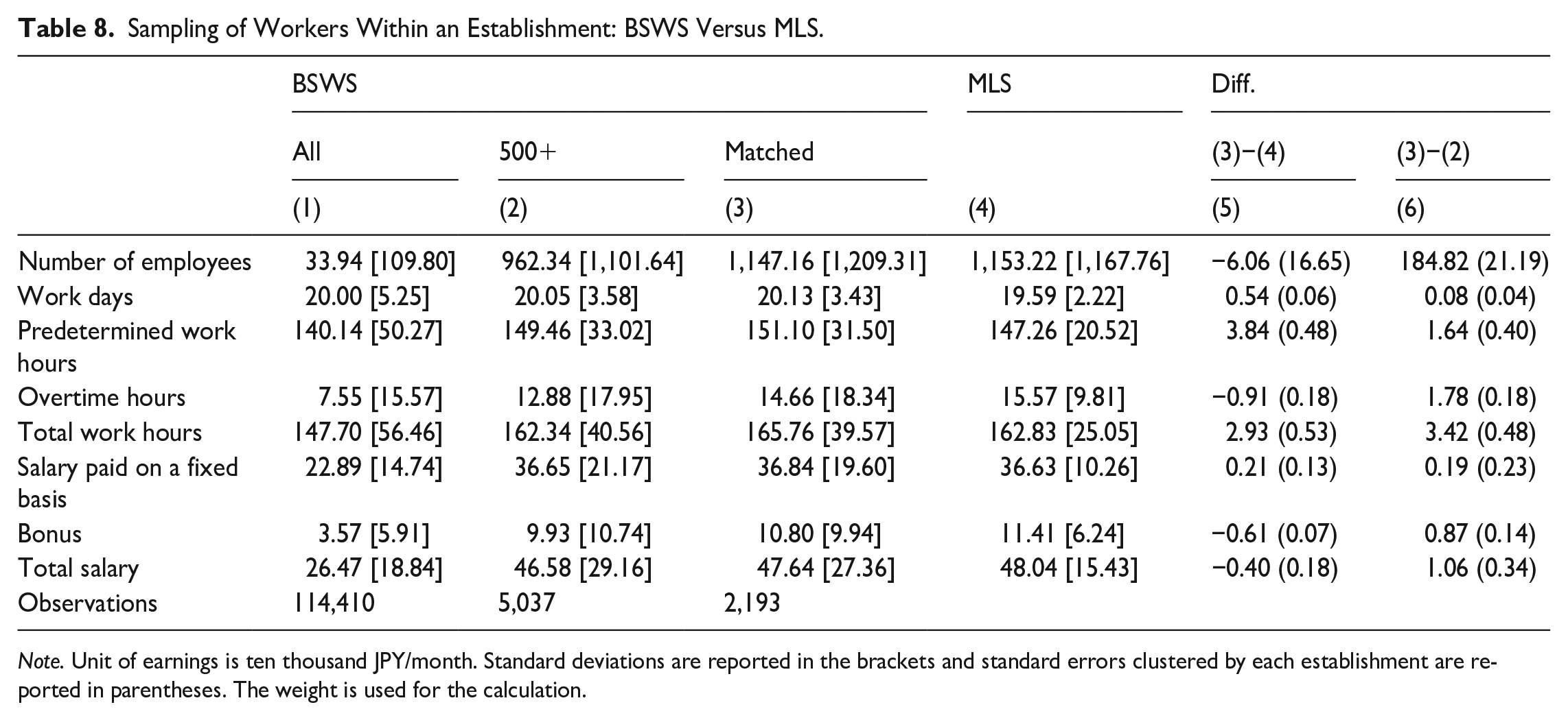
Note. Unit of earnings is ten thousand JPY/month. Standard deviations are reported in the brackets and standard errors clustered by each establishment are reported in parentheses. The weight is used for the calculation.

Compared to the grand mean reported in Column 1, employees of larger establishments tend to work longer and receive higher wages and bonuses, but limiting the establishment size does not essentially alter our conclusion because we are interested in the random sampling of workers within an establishment. Next, we match the 5,037 establishments in the BSWS from 2016 to 2017 with those in the MLS from 2016 to 2017 using the common establishment identifier. Although all establishments in the BSWS should also appear in the MLS, the number of establishments that can be successfully matched in this way is only 2,193, or 44% of the establishments in the BSWS. One partial explanation for the low match rate is the MHLW non-compliance with the MLS sampling design, which targets all establishments with 500 or more employees. However, in Tokyo prefecture, for example, only one-third were actually sampled. See Appendix C for characteristics of BSWS establishments that we are not able to match with the MLS.

Next, we compare the statistics of the BSWS establishments matched with the MLS (Column 3) and those of the MLS (Column 4). Since these statistics are from the same (matched) establishments, the means should be identical, and indeed, there is no statistically or economically significant difference in the number of workers. As this variable is establishment-level information (and not relying on the sampling of workers), it underpins our confidence that the two data sets are matched correctly.

Comparing other statistics, we note that the number of working days and working hours is about 2 to 3% higher for the BSWS, and while there is no difference in regular salaries, bonuses are slightly higher in the MLS. This brings the total salary, defined as the sum of the salary paid on a fixed basis and 1/12 of the annual bonus, about four thousand JPY higher in the MLS, which is statistically significant but less than 1% of the average value. ¹ In the end, we conclude that average hours worked and wages calculated based on the randomly selected individual employees in the BSWS and the aggregate statistics in the MLS are not substantially different in any economically meaningful way. This suggests that the random sampling of employees that was delegated to the employer was conducted properly, though not perfectly, at least to the extent that the mean wages are unbiased estimates. Additionally, when we investigate the sampling of workers by gender, we similarly find a bias in earnings across gender, with the magnitude statistically significant but not economically meaningful. Specifically, the earnings of male (female) sampled workers in the BSWS tend to be lower (higher) than those in the MLS. See Appendix E for details.

A caveat of this analysis is that it applies only to large establishments with 500 or more employees, and from this analysis we cannot rule out the possibility that smaller establishments fail to randomly sample their workers. Due to the low match rate of the BSWS and MLS, the analysis for establishments with less than 500 employees is not feasible, so we instead use the SSPS to investigate heterogeneity by establishment size because the same analysis can be conducted for the SSPS without matching other survey data, as described below. The results of the analysis show that small establishments are more likely to conduct random sampling inappropriately, but the resulting size of the bias is at most 3.4% (Table G5).

5.2. The Statistical Survey of Actual Status for Salary in the Private Sector

We now move on to examining the random sampling of employees within an establishment based on the SSPS. As the SSPS requires establishments (tax withholding agents) to report the number of salaried workers and the wage bill (the total amount of salaries paid), we can directly calculate the mean annual earnings per worker without matching it to other statistics. At the same time, we can calculate the corresponding figure using the sampled employees. If the sampling of employees is random, as per the survey design, then the mean annual salary based on the establishment (tax withholding agent) form should coincide with that of the worker (payroll income) form.

As a first cut, Figure 2 plots the distribution of annual earnings from each questionnaire, pooling data from 2012 to 2019. In this figure, the blue bars show the distribution of average annual salaries, which is calculated by taking the average of salaries of workers selected in the Worker form by each establishment. Meanwhile, the red bars show the distribution of salaries per worker, which is calculated by dividing the total payroll by the average number of employees in March, June, September, and December using the Establishment form. The overlap of the two distributions reassures us that the random sampling of employees within an establishment conducted by employers is implemented properly. There are, however, several notable irregularities. First, the figure shows that a non-negligible proportion of workers earn less than JPY 50,000 in the distribution calculated from the worker questionnaire. This might have occurred because salaried employees who worked only a few months of the year were sampled, and their annual earnings would be lower because of the fewer annual hours worked. Second, the distribution calculated from the data on the establishment form shows a slightly larger number of people earning JPY 20 million or more. The data from the establishment form sometimes shows extremely high values, and one reason for this may be that in order to calculate the payroll per employee, the total payroll is divided by the “average” number of employees measured quarterly. In particular, measurement error in the number of employees would not be negligible in establishments whose labor demand has substantial seasonality, and in some cases, this measurement error might lead to artificially high earnings per worker. With these caveats, the distributions of annual earnings based on the establishment and worker surveys are reasonably similar.

Figure 2.

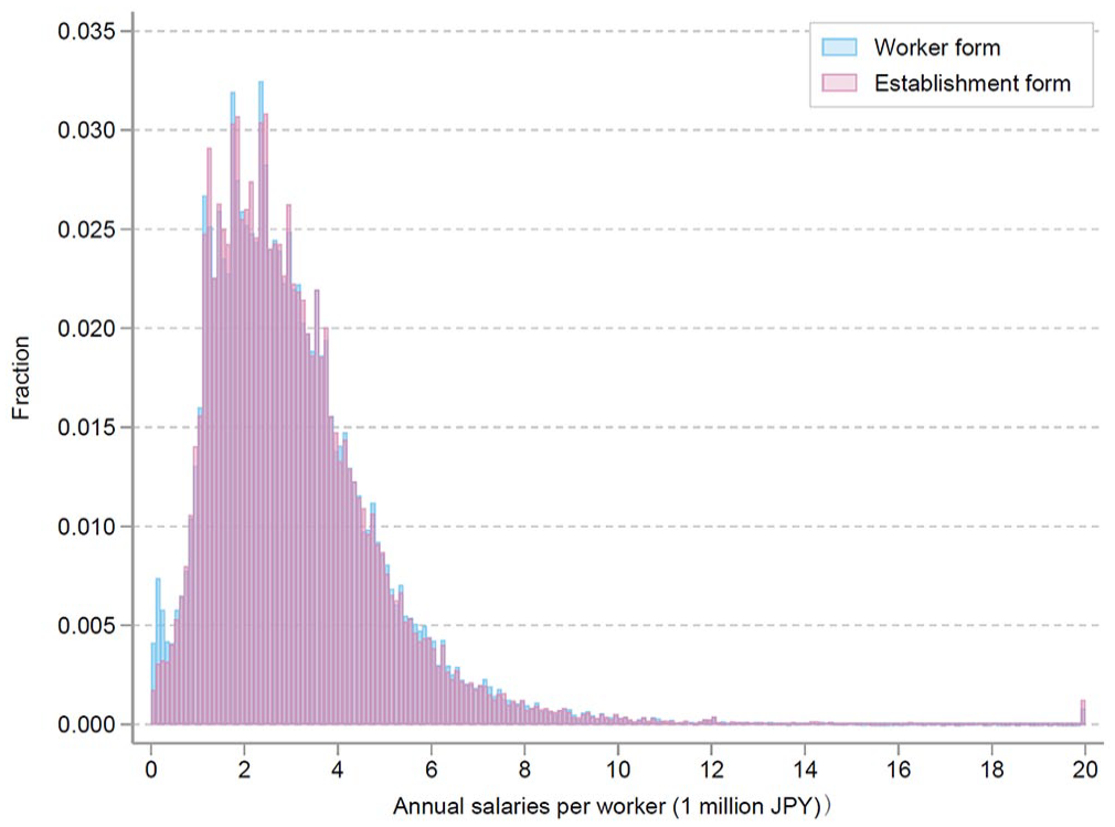
The distribution of mean earnings by establishments (SSPS, Unit: 1 million JPY/year).

We next compare the distribution of mean annual wages calculated based on establishment-level aggregates and randomly selected individual payroll records, focusing on the means and other percentiles (Table 9). We see that the mean calculated from the worker form is JPY 100 and JPY 50,000 lower than the mean from the establishment form. Looking at the percentiles, low percentile values are lower and high percentile values higher in the worker form, which indicates that the mean of the establishment-level annual earnings based on the worker form has a wider distribution than the one based on the establishment form. However, compared to the difference in means, the differences in percentile values are more limited. The reason for the large difference in the mean but small difference throughout the distribution is that, as mentioned above, the earnings per worker calculated from the establishment questionnaire may be affected by a small number of outliers. In fact, we find that only a few records have a substantial impact. When the top and bottom 1% of records are trimmed, the difference in the mean shrinks substantially (Columns 4–6 of Table 9). Although the difference in the mean is statistically significant, its magnitude is negligible at JPY 9,000 or 0.3% of the mean. Meanwhile, as the percentile values are not affected by outliers, the results are almost identical irrespective of the treatment of outliers.

Table 9.

Sampling of Workers Within an Establishment: SSPS.

Questionnaire	All			Non outliers
	Worker	Establishment	Diff. (1)−(2)	Worker	Establishment	Diff. (4)−(5)
	(1)	(2)	(3)	(4)	(5)	(6)
Mean	3.067 [2.000]	3.220 [19.988]	−0.153 (0.090)	3.039 [1.897]	3.030 [1.866]	0.009 (0.002)
p10	1.181	1.201	−0.020 (0.003)	1.188	1.201	−0.013 (0.004)
p25	1.775	1.787	−0.011 (0.004)	1.777	1.781	−0.004 (0.004)
p50	2.703	2.697	0.006 (0.004)	2.692	2.681	0.011 (0.004)
p75	3.903	3.872	0.030 (0.006)	3.870	3.840	0.030 (0.005)
p90	5.316	5.253	0.063 (0.010)	5.251	5.169	0.081 (0.009)
Observations	163,993	163,993	163,993	157,661	157,661	157,661

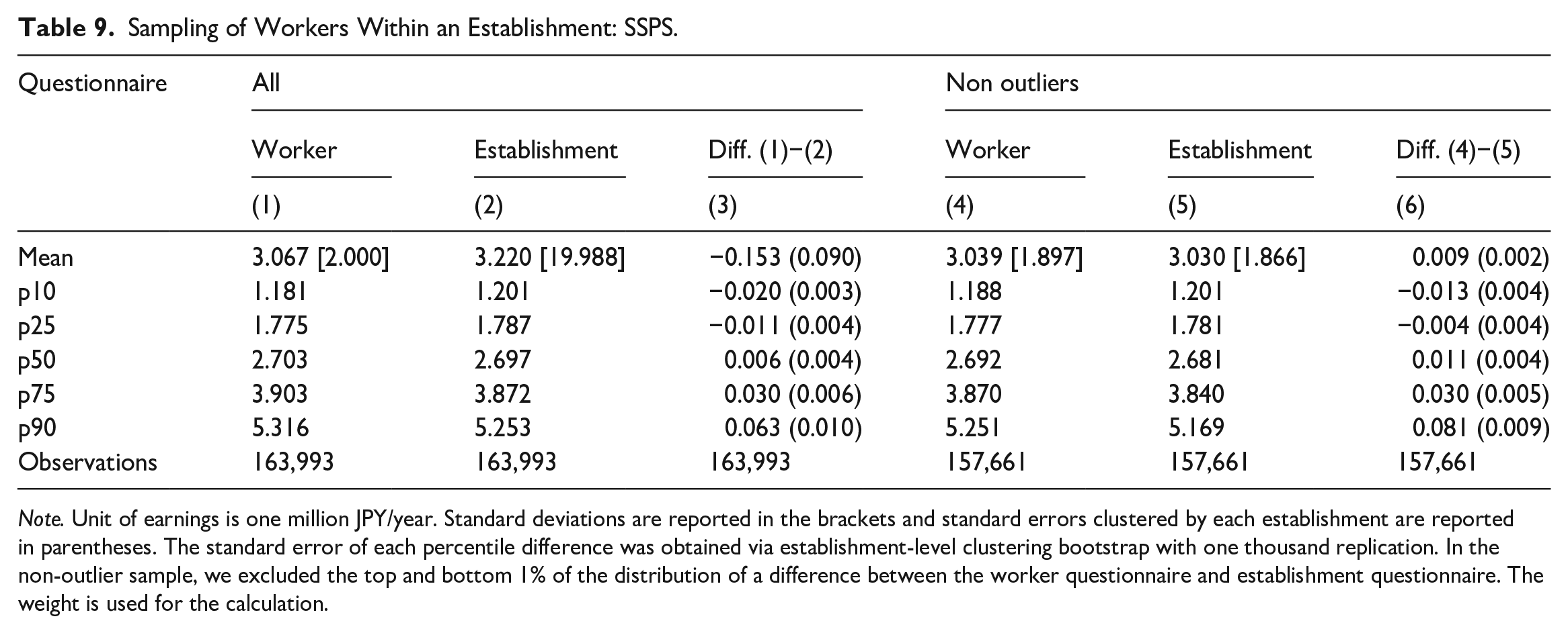
Note. Unit of earnings is one million JPY/year. Standard deviations are reported in the brackets and standard errors clustered by each establishment are reported in parentheses. The standard error of each percentile difference was obtained via establishment-level clustering bootstrap with one thousand replication. In the non-outlier sample, we excluded the top and bottom 1% of the distribution of a difference between the worker questionnaire and establishment questionnaire. The weight is used for the calculation.

In sum, both the BSWS and SSPS appear to perform the random sampling of workers adequately, for while we find some statistically significant biases in the sampling of workers, the magnitude is not economically meaningful. Thus, the impact of the non-random sampling of workers within an establishment seems very limited.

6. Uncovered Population

In the preceding analysis of bias associated with a given population for random sampling, we find that the size of the bias is negligible, at least when the estimation of wages is of interest. However, another important issue is the sampling frame, for if the sampling population is not representative of the entire population, the survey data would be biased relative to the entire population even with a 100% response rate. Thus, we now investigate the potential for such a mechanical bias due to the sampling design, as neither the BSWS or SSPS covers self-employed workers, which includes freelance workers. Given the heightened attention to the gig economy, or a labor market characterized by flexible and short-term labor contracts, and freelance workers for such services as Uber Eats, we attempt to document them by using a household survey that covers all workers regardless of the form of employment. In addition, the BSWS does not cover establishments with one to four employees and corporate executives, which are covered by the SSPS. In this section, we evaluate how the coverage of freelance workers and workers at small establishments affects the wage statistics, while the coverage of top-tier incomes are analyzed in Section 8.

6.1. Freelance Workers

Since the BSWS and SSPS do not cover freelance workers, we evaluate the impact of this limitation in coverage on wage statistics by using the Employment Status Survey (ESS). In this analysis, we regard freelance workers as self-employed workers who themselves do not have employees. We note that the definition of freelance workers might vary. For example, the Japan Cabinet Office excludes individual shopkeepers with a physical storefront as well as agricultural, forestry, and fishery workers from its definition of freelance workers. However, we emphasize that the objective of the analysis here is not to reveal the characteristics of freelance workers defined in a certain way but to reveal those of workers not covered by the main Japanese wage statistics, and freelance workers as defined here correspond to that population.

Although the proportion of freelance workers has been decreasing steadily, from 13% of the working population in 1977 to 6% in 2017 (Figure 3), the share of freelance workers among the self-employed is high at around 70% and has been increasing in recent years. According to the 2017 ESS, freelance workers are older, with a higher percentage of males, a higher rate of marriage and lower education, and they chose the current job in order to utilize their knowledge and skills (Tables F1 and F2). Table 10 shows that the earnings of freelance workers tend to be substantially lower than for other workers, with 24% of freelance workers earning less than JPY 500,000/year (Column 5) but only a small fraction (4.7%) of other workers earning that amount (Column 2). Furthermore, comparing Columns 2 and 5, we find that the income distribution of freelance workers is stochastically dominated by that of non-freelance workers, with the mean annual income, calculated using the mid-value of each income category, JPY 2.1 million for freelance workers and JPY 3.5 million for other workers. While the income gap between non-freelance and freelance workers is substantial, the small share of freelancers among the entire working population causes the Japanese mean income statistics to be upwardly biased by only 2.6% $\left(=100\times \frac{3.545-3.456}{3.456}\right)$ when freelance workers are not counted.

Figure 3.

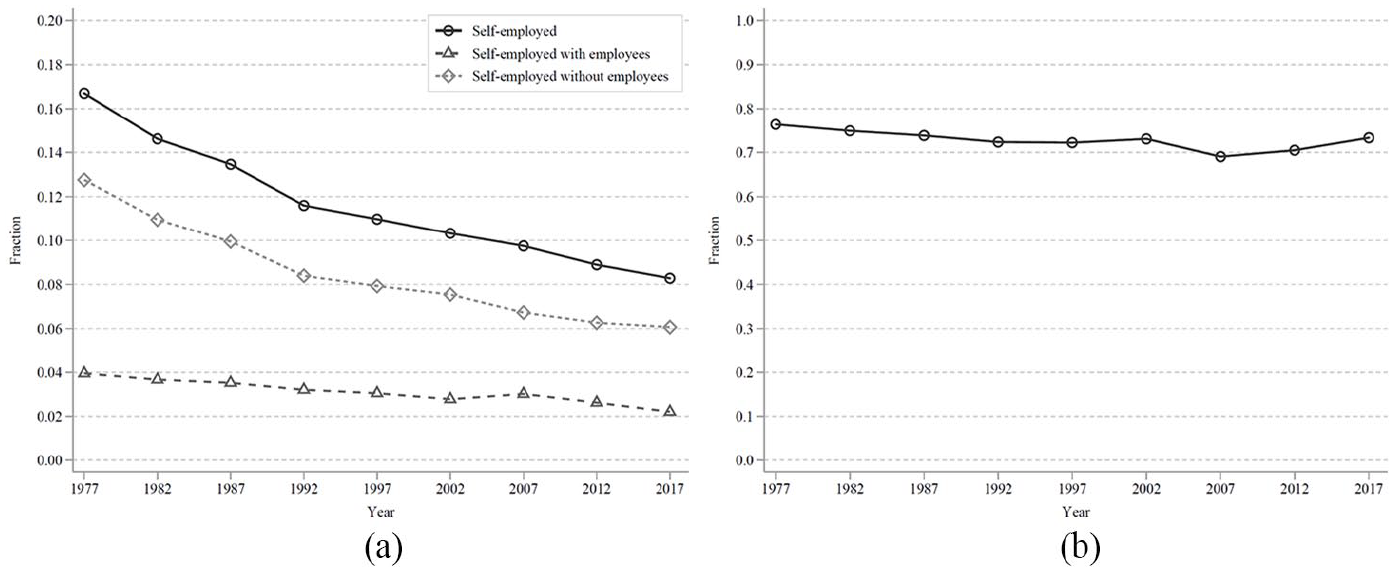
Proportion and composition of self-employed workers: (a) fraction of self-employed workers and (b) share of self-employed workers without employees among self-employed workers.

Table 10.

Income Distribution (ESS 2017).

	All	Non freelance	Employees	Self-employed
				Non freelance	Freelance
	(1)	(2)	(3)	(4)	(5)
Composition	1.000	0.939	0.917	0.022	0.061
Income distribution
0–0.5 million JPY	0.059	0.047	0.046	0.083	0.244
0.5–0.99 million JPY	0.114	0.112	0.113	0.066	0.147
1–1.49 million JPY	0.104	0.102	0.103	0.084	0.127
1.5–1.99 million JPY	0.075	0.074	0.074	0.080	0.087
2–2.49 million JPY	0.107	0.108	0.108	0.102	0.092
2.5–2.99 million JPY	0.080	0.081	0.081	0.078	0.067
3–3.99 million JPY	0.139	0.141	0.142	0.133	0.097
4–4.99 million JPY	0.100	0.103	0.103	0.092	0.052
5–5.99 million JPY	0.070	0.073	0.073	0.069	0.029
6–6.99 million JPY	0.048	0.050	0.050	0.039	0.017
7–7.99 million JPY	0.035	0.037	0.037	0.027	0.012
8–8.99 million JPY	0.022	0.023	0.023	0.023	0.007
9–9.99 million JPY	0.014	0.014	0.014	0.020	0.005
10–12.49 million JPY	0.020	0.020	0.020	0.039	0.007
12.5–14.99 million JPY	0.005	0.006	0.005	0.015	0.002
15 million JPY or more	0.009	0.009	0.008	0.051	0.004
Mean income (1 million JPY)	3.456	3.545	3.528	4.255	2.097

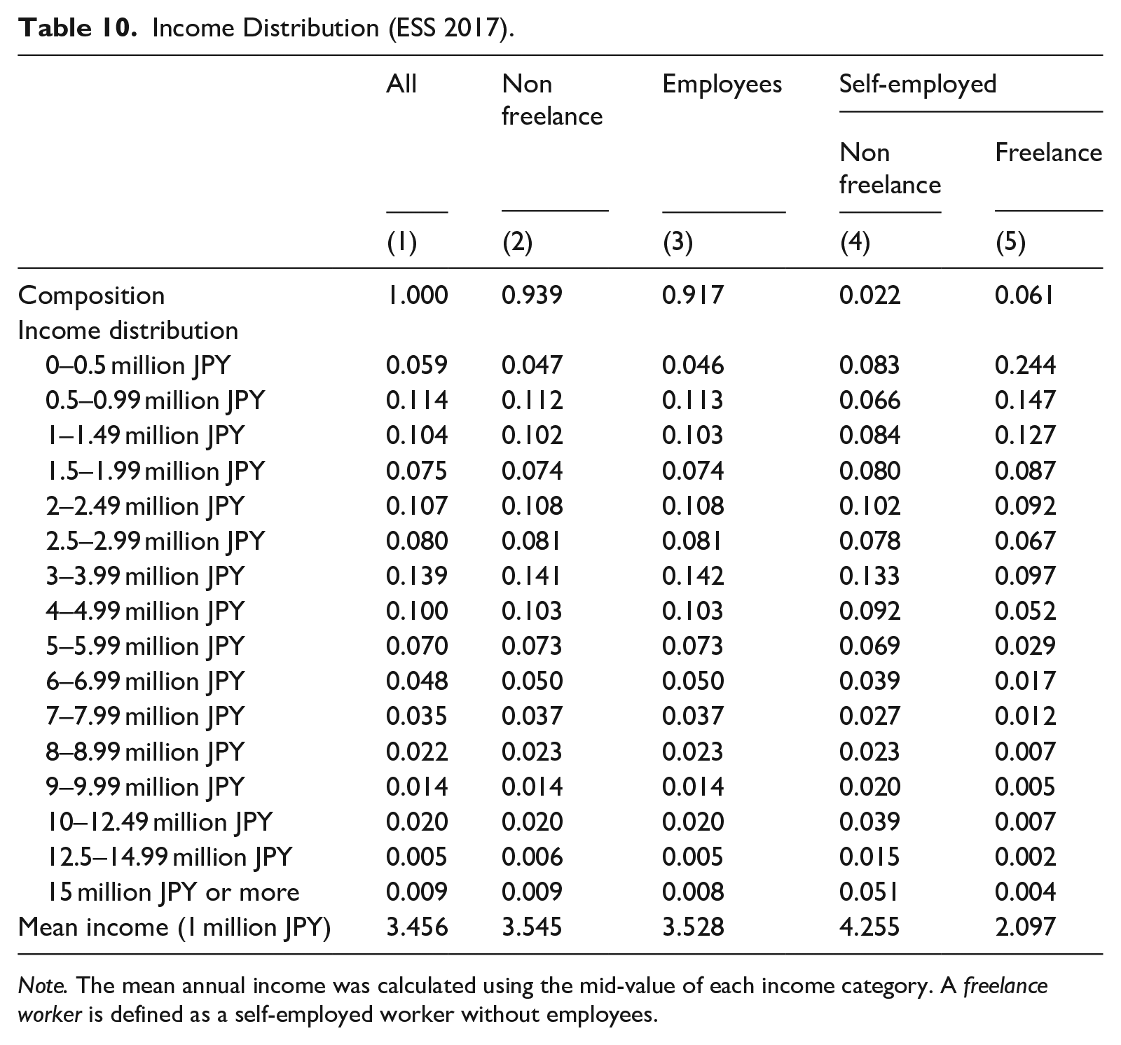
Note. The mean annual income was calculated using the mid-value of each income category. A freelance worker is defined as a self-employed worker without employees.

6.2. Small Establishments with One to Four Employees

We now move on to discuss the limited coverage of small establishments in the BSWS. This is acknowledged by policy makers and researchers as a limitation of the survey, who find the SSPS more suitable for characterizing the earnings of workers of micro establishments because it covers the entire population of withholding agents with one or more employees. Another, perhaps less known, limitation in the coverage of the BSWS is the exclusion of corporate executives. By contrast, the SSPS not only covers corporate executives but also instructs establishments to include every worker who earns JPY 20 million (about USD 200,000) or more annually. This top end of the wage distribution will be discussed in Section 8, but for our purposes here, it is important to note that the SSPS covers a wider range of workers than the BSWS. We next use the SSPS to describe the characteristics of workers not represented by the BSWS.

First, we characterize the employees of micro-scale firms and note that while the employee share of withholding agents with one to four employees is only 19%, they account for 83% of all withholding agents. Moreover, the characteristics of workers in those micro establishments are distinct from those of other workers (Table 11). In particular, workers in micro-establishments are more likely to be female (4.2percentage points higher), older (by 7.5 years), and with longer tenure (by 3.7 years). However, despite their higher age and longer tenure, their earnings are lower than workers in establishments with five or more employees, a difference of 9.4% in regular salary excluding bonuses, 69.2% in bonuses, and 19.4% in total earnings. When controlling for worker attributes (gender, age, and tenure), the difference in earnings expands to 17.7 and 25.1% in terms of regular salary and total earnings, respectively (Table 12).

Table 11.

Characteristics of Workers in Establishments with Four or Less Employees (SSPS).

Establishment size	1–4	5 or more	Diff. (1)−(2)	Frac. $\frac{(1)-(2)}{(2)}$
	(1)	(2)	(3)	(4)
Female	0.470 [0.499]	0.427 [0.495]	0.042 (0.003)	0.101
Age	50.902 [15.201]	43.439 [13.815]	7.463 (0.076)	0.172
Tenure	13.212 [13.175]	9.524 [10.295]	3.688 (0.077)	0.387
Salary excl. bonus	2.970 [3.033]	3.279 [3.200]	−0.309 (0.019)	−0.094
Bonus	0.202 [0.541]	0.655 [1.142]	−0.453 (0.008)	−0.692
Total salary	3.172 [3.185]	3.933 [3.859]	−0.762 (0.026)	−0.194
Observations	163,051	2,239,078

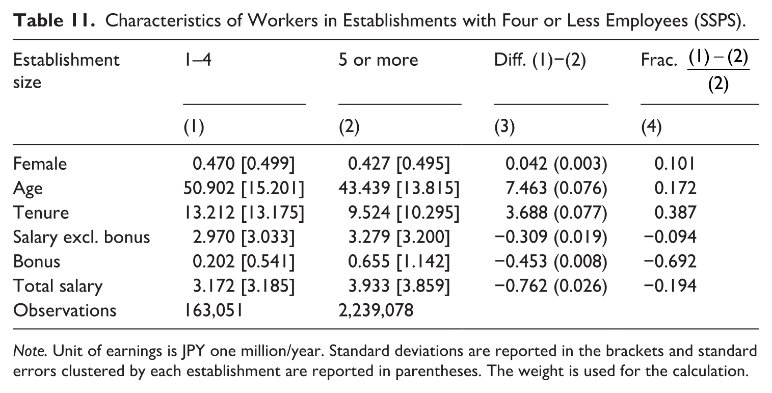
Note. Unit of earnings is JPY one million/year. Standard deviations are reported in the brackets and standard errors clustered by each establishment are reported in parentheses. The weight is used for the calculation.

Table 12.

Regression Analysis: Earnings in Establishment with Four or Less Employees.

Dep.Var.	ln (Salary excl. bonus)		ln (Total salary)
	(1)	(2)	(3)	(4)
Establishment size ≤4	−0.110 (0.008)	−0.177 (0.005)	−0.187 (0.009)	−0.251 (0.005)
Controls		X		X
Observations	2,402,114	2,402,114	2,402,114	2,402,114

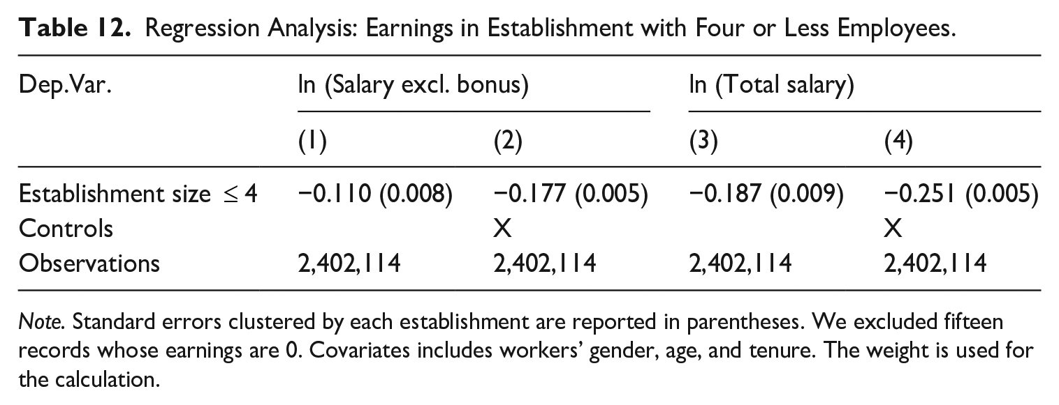
Note. Standard errors clustered by each establishment are reported in parentheses. We excluded fifteen records whose earnings are 0. Covariates includes workers’ gender, age, and tenure. The weight is used for the calculation.

The above analysis suggests that the BSWS, which is often used to describe the wage distribution in Japan, fails to adequately capture workers with low earnings. Compared to the figures from the SSPS, the BSWS does not cover 19% of employees whose earnings are, on average, 19.4% lower than the BSWS sample (as shown in Column 4 of Table 11). In the end, the bias associated with this uncovered population amounts to about 4%. This under-coverage of low-wage workers is, of course, of particular importance in the assessment of policies such as the minimum wage that targets low-wage earners. Neglecting these low-wage earners underestimates the proportion of workers who are affected by a minimum wage hike.

7. Overall Bias: Comparison with Administrative Records

A goal of a national wage survey is to understand the wage structure of the entire population. However, the BSWS and SSPS have two potential issues: nonresponse bias and coverage as discussed in Sections 4 and 6, respectively. While due to data limitations we conducted the analyses by imposing some assumptions which allowed us to make inferences about those not responding to the survey, a preferred way to examine the representativeness of the survey data in terms of the entire population is to link the survey data with administrative payroll data, as performed by Phipps and Toth (2012) for example. Unfortunately, access to national administrative data that can be merged with the BSWS or SSPS is not available in Japan. However, we were able to access administrative tax record data of a city of about one million residents located in the Kyushu region. Since the SSPS does not record the location of establishments, we compare the tax record data to the BSWS wage distribution in that city. One limitation of this analysis is that we cannot match data at an individual or an establishment level. Further, location in the BSWS is based on the location of the establishment whereas location in the tax data is that of a worker’s residence, so the population of the BSWS is not identical to that of the tax data to the extent that there are inter-city commuters.

With this caveat in mind, Table 13 shows the distribution of annual earnings based on the BSWS and the tax data in 2017. Consistent with the limited coverage of the BSWS as discussed in Section 6, the BSWS substantially over-estimates the 25th percentile and below, and under-estimates the 75th percentile and above. In particular, the bias at the lower tail of the distribution is tremendous. For example, earnings at the 5th percentile in the BSWS are almost double that of the tax data, and the bias at the 10th and 25th percentiles is more than 30%. By comparison, the bias at the top of the distribution, while not negligible, is relatively mild with a magnitude of 10 to 13%. Given that the share of workers in small establishments and freelance workers is larger than the share of corporate executives, this pattern seems well-explained by the limited coverage of the BSWS, though we cannot rule out the possibility that unit nonresponse bias is particularly serious at the tails of the earnings distribution in this city.

Table 13.

Distribution of Annual Earnings: The BSWS Versus the Administrative Tax Data.

	BSWS	Tax data	Diff. (1)−(2)	$\%\Delta$ : 100 $\times \frac{(3)}{(2)}$
	(1)	(2)	(3)	(4)
Mean	3.691 (0.048)	3.863 (0.008)	−0.172 (0.049)	−4.46
p5	0.862 (0.031)	0.436 (0.005)	0.426 (0.031)	97.65
p10	1.094 (0.036)	0.796 (0.004)	0.298 (0.036)	37.50
p25	2.161 (0.039)	1.611 (0.008)	0.551 (0.040)	34.18
p50	3.252 (0.054)	3.340 (0.009)	−0.088 (0.055)	−2.65
p75	4.586 (0.059)	5.200 (0.011)	−0.614 (0.060)	−11.81
p90	6.437 (0.151)	7.424 (0.015)	−0.987 (0.152)	−13.30
p95	7.971 (0.175)	8.782 (0.023)	−0.811 (0.175)	−9.24
Observations	6,402	160,529

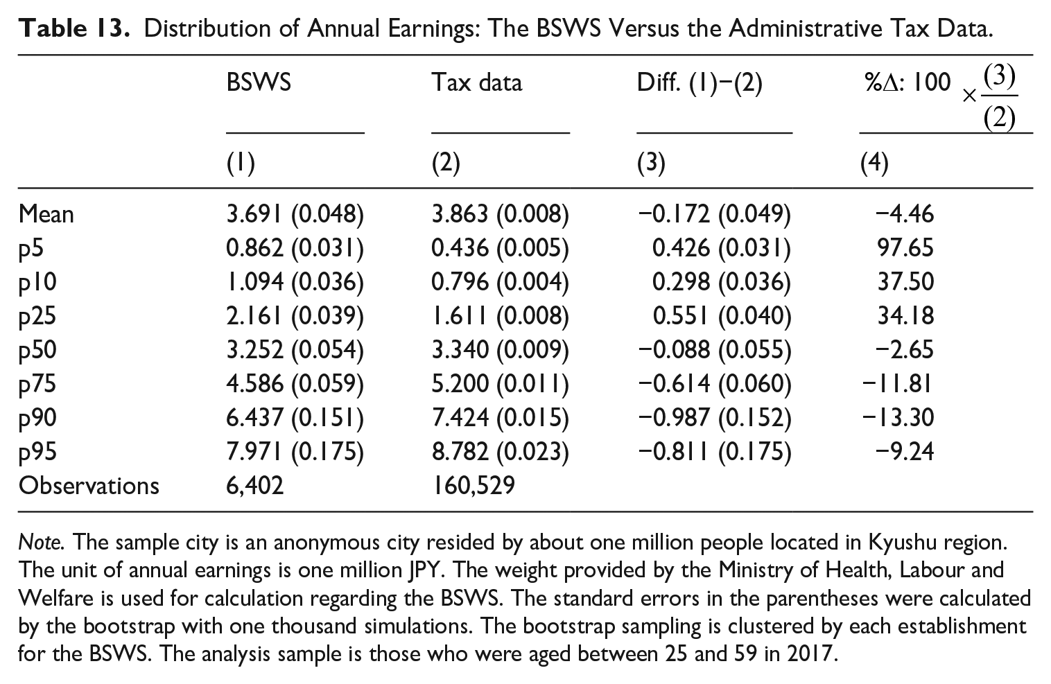
Note. The sample city is an anonymous city resided by about one million people located in Kyushu region. The unit of annual earnings is one million JPY. The weight provided by the Ministry of Health, Labour and Welfare is used for calculation regarding the BSWS. The standard errors in the parentheses were calculated by the bootstrap with one thousand simulations. The bootstrap sampling is clustered by each establishment for the BSWS. The analysis sample is those who were aged between 25 and 59 in 2017.

However, in contrast to the tails of the earnings distribution, the difference between the BSWS and the tax data at the mean and median is small. Although the mean of the BSWS is statistically significantly lower than that of the tax data, the magnitude of the difference is limited to 4.5% (Row “mean” in Column 4). Since the mean is particularly vulnerable to the upper tail of the distribution, the under-estimation of the mean might be attributed to the under-estimation of the upper tail. Consistent with this argument, we do not find a statistically significant difference in the median, which is less vulnerable to the tails of the distribution. Furthermore, the magnitude of the difference in the median is only 2.7% (Row “p50” in Column 4). Therefore, this case study indicates that the BSWS is still useful for understanding the population mean or median wage despite its limited coverage.

To summarize, this case study casts serious doubt on the estimation of the tails of the population wage distribution using the BSWS presumably due to its limited coverage, and the bias is particularly severe at the very bottom of the distribution. On the other hand, the BSWS provides a good estimate of the population’s mean and median wage. Finally, we note that this result is based on the analysis of only one city, and one needs to be careful when generalizing this result to the overall Japanese population because the coverage rate of the population is a key determinant of the bias and this could substantially differ across cities. Future research aims to collect the administrative records in other cities as well to examine the external validity of the result we have found here.

8. Application: The Evolution of Wage Inequality

As an example of how this difference in the coverage of the BSWS and SSPS may affect real-world policy-making, we investigate its impact on the depiction of the evolution of wage inequality. We first examine the evolution of the lower end of the income distribution, and Figure 4a shows the 10 to 50 percentile ratio using the BSWS and the SSPS. According to the long-run trend from the BSWS, the ratio decreased in the late 1990s and early 2000s, particularly among females, but has been stable in recent years. Since the SSPS covers small establishments not covered by the BSWS and since small establishments tend to pay less, the gap becomes larger when using the SSPS, but the time-series trends are similar. Panel A of Table G6 statistically tests if the annual growth rates of the ratio of the BSWS and SSPS are different, and we find that the difference is not statistically significant except for 2013. As a caveat, we note that our time series for the SSPS is too short to conclude if their trends are in fact comparable.

Figure 4.

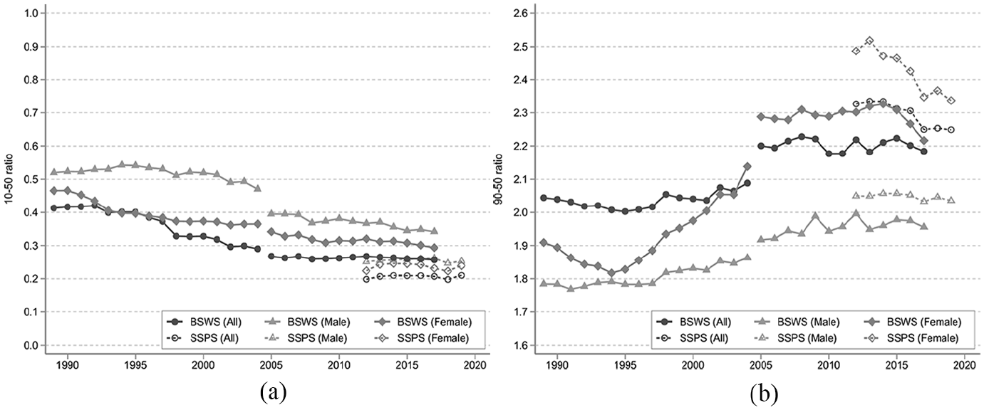
Wage inequality: (a) 10 to 50 percentile ratio and (b) 90 to 50 percentile ratio.

We now move our focus from the lower tail to the upper tail of the wage distribution. While the BSWS covers only workers and not corporate executives, the SSPS covers all salaried workers including corporate executives and, furthermore, the SSPS design calls for sampled establishments to report salary information for all employees whose annual salary exceeds JPY 20 million. As a result, the SSPS captures the right tail of the income distribution more accurately. Next, we investigate to what extent inequality measures differ between the BSWS and the SSPS.

Figure 4b shows the 90 to 50 percentile ratio of the earnings distribution. According to the BSWS, the 90 to 50 ratio has been relatively stable over the last few decades, though there was a discrete jump in 2005 due to a change in the sampling design, with the 90th percentile about twice as large as the median. The ratio increased from the 1990s and early 2000s for both males and females, but was particularly striking for females, before becoming relatively stable after 2005 for both. Since the SSPS has more complete coverage of the upper tail of the income distribution, the 90 to 50 percentile ratio is larger than that of the BSWS, but the difference is at most 10%. Furthermore, in terms of the yearly trend, the BSWS appears to again track the SPSS trend well, notwithstanding the SSPS limitation of a shorter time series (Panel B in Table G6). The small difference in the 90 to 50% ratio between these two surveys is probably because the uncovered population in the BSWS; namely, executives, lies at the very top of the income distribution and so they have limited impact on the 90th percentile.

In order to focus on the very top end of the income distribution, we next calculate the top 1 and 0.1% earnings shares (Figure 5). The BSWS shows relatively stable trends, though the top 1% share increased slightly during the 2000s. In contrast to the BSWS, the SSPS indicates that the top income share increased during the 2010s, with the top 1% share growing from 5.8 to 6.3%, and the top 0.1% share growing from 1.2 to 1.6% (See Tables G7 and G8 for the statistical test for the annual growth rate of the top income share). Moriguchi and Saez (2008) and Alvaredo et al. (2012), who estimate the right tail of the income distribution by fitting a Pareto distribution to the binned tax data and the estimated Pareto coefficient, calculate the top income share in Japan between 1886 and 2010. According to their estimates, the top 1 and 0.1% shares were 9.5 and 2.5% in 2010. These estimates are larger than ours, and we suspect that the difference is due to how income is defined, for they include non-labor income such as rent, interest, and dividends while our income is limited to labor income. Moriguchi and Saez (2008) do disentangle total income into these detailed income categories and find that the top 1% share of employment income to be about 7% in 2005, which is more in line with our estimates.

Figure 5.

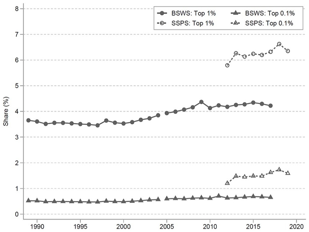
Top income share.

As performed in Moriguchi and Saez (2008) and Alvaredo et al. (2012), another method to illustrate the top income distribution is to estimate the Pareto distribution:

$$F(y)=1-{\left(\frac{y_m}{y}\right)}^{\alpha }(y\ge y_m),$$

(14)

where $y_m$ is some threshold parameter and α is a parameter that characterizes the tail of the income distribution, with a smaller value of α meaning a fatter right tail. In other words, a small value for α indicates substantial inequality among high-income individuals. In particular, when $\alpha \le 1$ , the distribution does not have a mean, and when $\alpha \le 2$ , the distribution does not have a variance. Following Atkinson et al. (2018), Equation (14) is rewritten as

$$\ln y=C+\frac{1}{\alpha }\ln \frac{1}{1-F(y)},$$

(15)

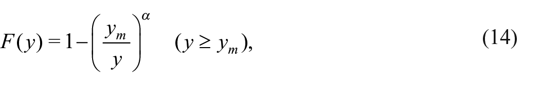
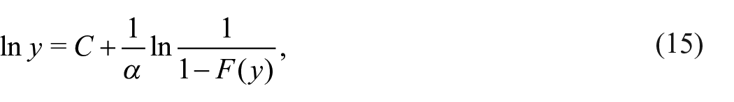
where C is some constant consisting of α and $y_m$ . We estimate this equation using those whose annual income was JPY nine million or more, which corresponds to the 95th percentile of the income distribution of both the BSWS and SSPS. Figure 6 shows that the Pareto coefficient obtained from the BSWS is larger than that of the SSPS, which implies that the SSPS captures upper tail inequality better than the BSWS. In addition, the SSPS estimates have smaller standard errors, indicating that the SSPS estimate is also more precise (Table G9). Furthermore, in terms of the Pareto coefficient, we find a clear difference in the trend observed in the BSWS and SSPS (Column 5 in Table G9). On the other hand, the difference between men and women is limited in both surveys. We note that the World Inequality Database provides the Pareto coefficient estimated from the binned income tax data, and its estimate for the 2010s is 2, which is smaller than ours, indicating more income inequality. As discussed above, this seems reasonable because the World Inequality Database includes capital income, while we do not. Recently, Kunieda and Yoneta (2023) report that the Pareto coefficients are 1.95 for labor income and 1.65 for capital income using micro-data of tax file, setting the lower bound of each income at JPY 200 million. Thus, both BSWS and SSPS underestimate the upper tail inequality.

Figure 6.

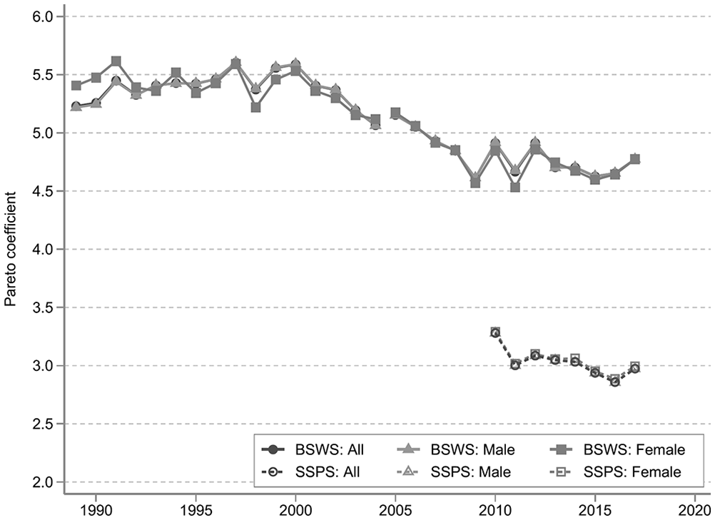
Pareto coefficient.

To summarize, the limited coverage of the BSWS leads to an under-estimation of wage inequality but yet it still picks up the overall trend, so the BSWS seems still useful as long as one is not interested in the absolute level but in the trend in income inequality. However, the bias of the BSWS could be serious when the very top of the income distribution is concerned.

9. Conclusion

In our investigation of the unit nonresponse biases of two representative large-scale national wage surveys, we find evidence of systematic heterogeneity in the unit nonresponse rates across industries, establishment sizes, and regions. In addition to these observed establishment characteristics, we analyze the relationship between survey response behavior and unobserved characteristics using the short-panel structure of the surveys, demonstrating that the relationship between survey response behavior and current wages can be approximated by past wages under the assumption of an auto-regressive process for wages. Our results show that the correlation between nonresponse risk and past wages is statistically significant but economically negligible. To evaluate the size of the unit nonresponse bias, we construct a new weight that separates nonresponse due to observed and unobserved characteristics but find that the magnitude of the bias is, at most, minor in both surveys.

Since the above analysis is drawn on the sample of establishments responding to the survey at least once, it is silent about sampled establishments that never responded to the surveys. To handle this issue, we assume that the wage distribution of never-responding establishments is similar to that of difficult-to-reach establishments, or those that only responded to the survey once even though they were sampled multiple times. The result of the analysis suggests that the nonresponse nonresponse bias is not economically meaningful at the mean and median but could be severe at the lower and upper tails of the wage distribution.

Beyond unit nonresponse bias, our analysis shows that the random sampling of workers by sampled establishments was conducted appropriately. This result is particularly useful for those who collect worker information with cluster sampling by establishments because the survey administrator typically does not have a list of workers in a given establishment in advance and thus it is difficult to randomly sample workers directly. In sum, we find that with proper weighting, nonresponse bias is negligible in national Japanese wage statistics to the extent that the mean estimate is concerned.

Although we find sampling bias to be negligible, we do find that the limited coverage of the sampling population of the BSWS leads to severe bias particularly at the tails of the wage distribution of the entire population. Indeed, when we compare the BSWS with the administrative tax records of one Japanese city, the bias at the 5th percentile is almost 100%, at the 10th and 25th percentiles is more than 30%, and at the 75th to 95th percentiles is around 10%. This finding has implications for the measurement of wage inequality based on the Basic Survey of Wage Structure (BSWS) that has been widely used in the literature (Kambayashi et al. 2008; Shinozaki 2006). We have shown that the BSWS under-samples both the lower and upper tails of the wage distribution compared to an alternative survey, the Statistical Survey of Actual Status for Salary in the Private Sector (SSPS). As a result, wage inequality is underestimated when using the BSWS, and this underestimation is particularly substantial when estimating the top of the income distribution. Despite the SSPS being less popular than the BSWS among researchers, our analysis demonstrates that the SSPS better serves the purpose of examining the tails of the wage distribution than the BSWS. This finding also suggests that administrative tax records are indispensable for examining behavior at the tails of the wage distribution. Furthermore, for a more complete characterization of the unit non-response bias over the wage distribution, administrative data that can be merged with the survey data at an individual level is required.