Bayesian Inference for Repeated Measures Under Informative Sampling

Abstract

Survey data are often randomly drawn from an underlying population of inferential interest under a multistage, complex sampling design. A sampling weight proportional to the number of individuals in the population that each sampled individual represents is released. The sampling design is informative with respect to a response variable of interest if the variable correlates with the sampling weights. The distribution for the variables of interest differs in the sample and in the population, requiring correction to the sample distribution to approximate the population. We focus on model-based Bayesian inference for repeated (continuous) measures associated with each sampled individual. We devise a model for the joint estimation of response variable(s) of interest and sampling weights to account for the informative sampling design in a formulation that captures the association of the measures taken on the same individual incorporating individual-specific random-effects. We show that our approach yields correct population inference on the observed sample of units and compare its performance with competing method via simulation. Methods are compared using bias, mean square error, coverage, and length of credible intervals. We demonstrate our approach using a National Health and Nutrition Examination Survey dietary dataset modeling daily protein consumption.

1. Introduction

Survey designs for sampling an underlying population of inference often consist of one or more stages to sample clusters of units, followed by the sampling of units. Unequal probabilities of selection are constructed to over-sample some individuals, often to reduce the variance for a domain estimator of interest. A sampled individual who responds to the survey is referred to as a survey participant, or, for simplicity in the sequel, a participant. Inference about the study population needs to consider the sampling design, in particular by incorporating sampling weights into the statistical analysis. Each individual, $i$ , in the population corresponds to a sampling weight, $w_i$ , that is designed to be inversely proportional to the joint inclusion and response probability, πi, of the individual $i$ as a participant; that is, the individual is selected and responded to the survey. We express this probability mathematically with,

$$\mathrm{Pr}[\mathrm{individual}i\mathrm{in}\mathrm{the}\mathrm{population}\mathrm{becomes}\mathrm{a}\mathrm{participant}]\propto {\pi }_i\propto 1/w_i$$

(1)

The weights are, therefore, adjusted for unequal selection probabilities of selection into the survey and for nonresponse, for example, when a selected individual declines to participate. The weights may also be adjusted for other situations; for example, in The National Health and Nutrition Examination Survey (NHANES) dietary datasets released for cycle 2003 to 2004 and later cycles, the dietary sampling weights are adjusted for the day the survey was taken (weekday vs. weekend). We take the perspective of secondary analysts, who are given the weights which are likely to include a nonresponse adjustment by the data producer. In secondary analysis no distinction between sampling and survey response weights is possible and one has to work with the associated unit-level weights. We note that we construct πi for our modeling in the sequel to be proportional and not necessarily equal to the marginal probability of becoming a participant and, thus, πi can take any positive value.

Let $y_i$ be the response variable of interest of the individual $i$ in the population. A sampling design is informative with respect to the response variable when the event of becoming a participant and the outcome is related even after conditioning on relevant characteristics of the individual, ${\mathbf{v}}_i$ , which is expressed mathematically by, $y_i\cancel{\perp }{\pi }_i|{\mathbf{v}}_i$ . León-Novelo and Savitsky (2019), hereafter referred to LS2019, propose a model-based Bayesian approach that specifies a joint likelihood for the sampling weights and the response variable of interest to correct for informative sampling. Their approach models the participant probabilities, πi and the response, $y_i$ , jointly via $p(y_i,{\pi }_i|\theta ,\kappa )=p(y_i|\theta )p({\pi }_i|y_i,\kappa )$ , where $p(y_i|\theta )$ is the distribution of the response in the study population and $\theta$ is the vector of population parameters of interest, while $\kappa$ the vector of nuisance parameters used to model the relationship between $y_i$ and πi and serves as an indicator of informativeness for the sampling design (to the extend that the credible interval [CI] for ${\kappa }_y$ , an entry of $\kappa$ defined below, is bounded away from 0). The target user for their model formulation to estimate $\theta$ in an unbiased fashion with respect to the population distribution is the data analyst who seeks to estimate the underlying generating parameters $\theta$ from data acquired from a survey sample. It is typical to provide the analyst values of the response variable and predictors for the survey participants along with the associated sampling weights. The approach assumes that the analyst knows the sampling weights and the predictor values for the participants only. The analysts knows neither the sampling weights nor predictor values for non-participants.

In LS2019 the main focus is linear regression with fixed effects. In this article, we extend their approach incorporating random effects in the linear regression model to accommodate repeated measures. Repeated measures arise when a response is measured multiple times for the same participant; for example, the NHANES dietary dataset consists of answers for the same dietary questionnaire at two different days for each participant. Our extension performed in this article incorporates the modeling for the association among the the measures within each participant. This is achieved by constructing participant-specific random effects (P-REs), $\delta$ , specified in the marginal linear regression model for the response variable (vs. the conditional model for the sampling weights given the response variable). We consider the case of continuous repeated responses.

The use of random effects to model the correlation among observations is common practice; for example, the NCI method (Tooze et al. 2002, 2006, 2010), which is the approach recommended to estimate typical (daily) nutrient intake when analyzing NHANES dietary data incorporates random effects. In particular, the NCI method is a generalized linear mixed effect model set-up where the correlation of the two repeated measures (i.e., participant nutrient intake in two different days) is modeled by a P-RE. They do not, however, include the sampling weights in their the statistical model. Instead, sampling weights are used to correct for the sampling design when fitting the model via a pseudolikelihood. The contribution of each observation to the log of this pseudolikelihood is proportional to the sampling weight, $\log \mathrm{pseudolikelihood}={\Sigma }_i{w}_i\log p\left(y_i|\theta \right)$ . Estimation consists of two steps: In the first step, the point estimates maximize the pseudolikelihood. These estimates are asymptotically unbiased. In the second step, confidence intervals for (and/or standard error of) the parameters are calculated via Taylor linearization or re-sampling methods (Centers for Disease Control [CDC] 2016b).

By contrast, our approach incorporates the sampling weights into the likelihood and no second step is required to compute credible intervals for the model parameters in order to achieve correct uncertainty quantification. Ours is the first formulation that incorporates P-REs into the model framework of LS2019.

The NCI method, by contrast, treats the weights as fixed in a “plug-in” formulation, which allows for noise unrelated to the response variable of interest for estimation. The plug-in approach is not fully Bayesian as is our joint modeling formulation such that the uncertainty relative to the distribution over all possible samples is not accounted for. LS2019 show that the pseudo or plug-in likelihood formulation produces overly optimistic or short credible intervals.

A class of pseudolikelihood approaches estimate the parameters of generalized linear mixed models under informative sampling by maximizing the log pseudolikelihood after integrating out the random effects. This approach parameterizes the so-called profile pseudolikelihood. Rabe-Hesketh and Skrondal (2006) propose adaptive quadrature to integrate out the random effects and focus on multistage sampling where random effects are used to model the dependence of units within the same cluster. They mainly focus on logistic regression. Later, Kim et al. (2017) propose an estimation method under informative two-stage cluster sampling. The approach in Kim et al. (2017) is based on approximating the profile pseudolikelihood using a normal approximation of the sampling distribution of the random effect estimates, avoiding integration of the random effects. Their focus is on linear and logistic regression, while here, ours is on linear regression only.

Their approaches further incorporate repeated measures for the same individual as we propose to do. Their methods use plug-in pseudolikelihood while ours, by contrast, is fully Bayesian using a likelihood defined for the observed sample, rather than approximate pseudolikelihood. Our approach focuses on the estimation of model parameters, $\theta$ , of the data generating model and not population totals (e.g., the population average of the response variable). A series of papers Zheng and Little (2003), Little and Zheng (2007), and Zangeneh and Little (2015) propose Bayesian methods to estimate population totals when the inclusion probabilities are proportional to a size variable. All of these approaches estimate the response value of non-sampled units to estimate the population total. By contrast, our approach utilizes only quantities available for sampled units.

In Section 2, we review the basic approach of LS2019. In Section 3 we introduce our extension that incorporates participant-specific random effects. In Section 4, we summarize the pseudolikelihood method and compare its performance with our fully Bayesian formulation in Section 5, in terms of bias, mean square error (MSE), and, coverage, as well as the length of credible intervals. In Section 6, we demonstrate our method with an NHANES dataset, estimating the daily protein consumption in the American population. We conclude with a discussion in Section 7. An Appendix presents details referred to, but not addressed in the main manuscript. We rely on Stan (Carpenter et al. 2016), which performs their No U-turns implementation of the Hamiltonian Monte Carlo posterior sampling algorithm, for estimation of Bayesian hierarchical model posterior distributions estimated in this article.

Going forward, the notation $\mathrm{normal}(\mu ,{\sigma }^2)$ is used to denote the normal distribution with mean m and variance ${\sigma }^2$ while $\mathrm{normal}(x|\mu ,{\sigma }^2)$ denotes its probability density function (PDF) evaluated at $x;\log \mathrm{normal}(\mu ,{\sigma }^2)$ denotes the lognormal distribution, so that $X\sim \mathrm{lognormal}(\mu ,{\sigma }^2)$ is equivalent to $\log X\sim \mathrm{normal}\left(\mu ,{\sigma }^2\right)$ and $\mathrm{lognormal}(x|\mu ,{\sigma }^2)$ the respective PDF evaluated at $x$ ; $MV{N}_p(\mathbf{m},\mathbf{S})$ denotes the p-variate normal distribution with mean vector $\mathbf{m}$ and variance-covariance matrix $\mathbf{S}$ ; and $\mathrm{gamma}(\mathrm{a},\mathrm{b})$ denotes the gamma distribution with shape $a$ and rate $b$ . Matrix, Iq, denotes the $q\times q$ identity matrix and ${\mathbf{1}}_q$ the $q$ dimensional column vector with all its entries equal to 1. All the non-transposed vectors are column vectors.

2. Review of LS2019 for Single Stage Designs

We next summarize the general formulation of LS2019 that focuses on a single stage of sampling with the model $(\theta ,\kappa )$ parameterized only using fixed effects. We extend and generalize this formation in the next section. Let $y_i$ be the response of the individual $i$ in the population and πi the corresponding inclusion probability, that is, the probability of s/he becoming a survey participant under the study sampling design (πi is inversely proportional to the sampling weight $w_i$ ). A sampling design is informative for inference on a participant response variable of interest when their inclusion probabilities are correlated with the response variable, $y_i\cancel{\perp }{\pi }_i$ for some $i$ .

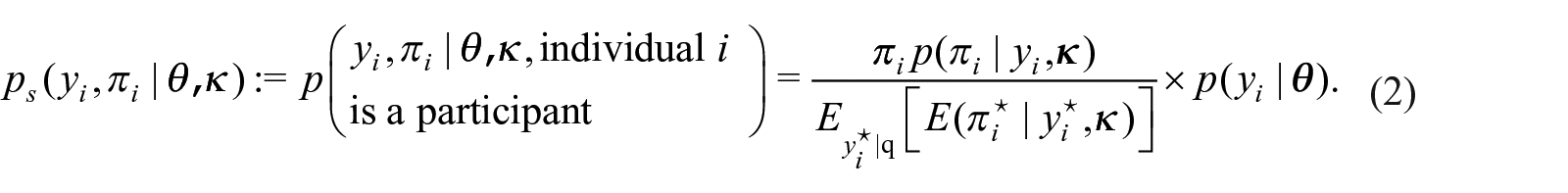
LS2019 introduce a Bayesian hierarchical construction that jointly models both the response, $y_i$ , and the marginal inclusion probability, πi, that is, $p(y_i,{\pi }_i|\theta ,\kappa )=p(y_i|\theta )\times p({\pi }_i|y_i,\kappa )$ , where $p(y_i|\theta )$ is the response or generating distribution for the population, $\theta$ is the population parameter of interest, and $\kappa$ is the nuisance parameter used to model the relationship between $y_i$ and πi that provides information on the degree of informativeness of the sample (based on how far the posterior credible intervals are bounded away from 0). LS2019 apply Bayes theorem (see derivation in Appendix A.1 or also Equation (7.1) in Pfeffermann et al. (1998)) to compute

$$p_s(y_i,{\pi }_i|\theta ,\kappa ):=p\left(\begin{array}{l}{y}_i,{\pi }_i|\theta ,\kappa ,\mathrm{individual}i\\ \mathrm{is}\mathrm{a}\mathrm{participant}\end{array}\right)=\frac{{\pi }_{i}p({\pi }_i|y_i,\kappa )}{E_{y_i^{\star }|\mathrm{q}}\left[E({\pi }_i^{\star }|y_i^{\star },\kappa )\right]}\times p(y_i|\theta ).$$

(2)

The superindex ⋆ denotes the quantity being integrated out. Note that the denominator in Equation (2) is the marginal probability of individual $i$ becoming a participant. The likelihood for the observed sample,

$$like(\theta ,\kappa )={\Pi }_{i=1}^n{p}_s(y_i,{\pi }_i|\theta ,\kappa ).$$

(3)

We note that for Equation (3) to be a valid likelihood we require

$$\begin{array}{l}\begin{array}{l}p\left[(y_1,{\pi }_1),\dots (y_n,{\pi }_n)|\mathrm{individuals}1\mathrm{to}n\mathrm{become}\mathrm{participants},\theta ,\kappa \right]\\ ={\Pi }_{i=1}^{n}p\left[(y_i,{\pi }_i)|\mathrm{individual}i\mathrm{becomes}\mathrm{a}\mathrm{participant},\theta ,\kappa \right]\end{array}\hfill \end{array}$$

(4)

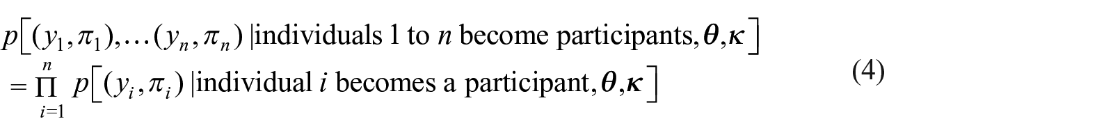
Appendix A.2 contains the proof that the following population and design conditions are sufficient for Equation (4):

• (C1) $(y_i,{\pi }_i)\stackrel{\mathrm{ind}}{\sim }p(\cdot |\theta ,\kappa )$ , with index $i$ running over population individuals, are independent. We construct the πis as unnormalized since a normalization would induce dependence (e.g., if we normalize such that the πs sum to 1, Pr(π2 > 0.5 | π1 > 0.6) = 0 and thus ${\pi }_1\cancel{\perp }{\pi }_2$ ).

• (C2) For any individual, conditioned on his/her response and inclusion probability, $\theta$ and $\kappa$ , the event of becoming a participant (being sampled and responding) is independent of any other individuals becoming participants, their responses and inclusion probabilities.

• (C3) Conditioned on $\theta$ and $\kappa$ , the response and inclusion probability of a population individual is independent of the responses and inclusion probabilities of the participants.

(C3) is natural in our framework, the responses and inclusion probabilities in the population are not affected by the ones in the sample (i.e., the participants). A referee noticed that in practice condition (C1) can be violated if the sampling weights, $w_i\propto 1/{\pi }_i$ , include nonresponse or post-stratification to known population totals adjustment (since the adjustment depends on the common data). For example, if Hispanics tend to have lower response rates, nonresponse adjustment will make their weights higher (and thus dependent), or if the proportion of Whites in the sample is higher than in the population post-stratification adjustment will make their weights lower. If this is the case the analyst is not receiving the πis as defined in Equation (1) but instead estimates of the πis that may be dependent. Yet, as secondary analysts we treat these estimates as if they were indeed the independent πis (despite adjustments for nonresponse and calibration). To cope with this case of dependent (estimated) inclusion probabilities, one can control for the variables used for adjustment (in our example race/ethnicity) when defining the distribution of ${\pi }_i|y_i,\kappa$ such that responses are independent conditioned on $\kappa$ (as we will discuss below after Theorem 1). (C2) is satisfied when sampling is with replacement and non adaptive (i.e., the probability of inclusion does not change by the observed values) but not satisfied when sampling is without replacement from a finite population. Nevertheless, if the population size is much larger than the sample size we can, as it is common practice, approximate the likelihood under sampling without replacement by the likelihood with replacement. When (C1), (C2), and (C3) hold in Equation (3) is a likelihood and the posterior distribution of the model parameters is

$$p_s\left(\theta ,\kappa |\mathrm{data}\right)\propto like\left(\theta ,\kappa \right)\times Prior\left(\theta \right)\times Prior\left(\kappa \right)$$

where $\mathrm{data}=\left\{(y_i,{\pi }_i):i=1,\dots ,n\right\}$ denotes the sample of size $n$ . Note that without loss of generality, the population individual index $i$ runs from 1 to n in the sample. The formula above allows fully Bayesian inference of the model parameters. The price the modeler pays for this fully Bayesian approach is the requirement to specify a conditional distribution of the inclusion probabilities for all units in the population, $p({\pi }_i|y_i,\kappa )$ , and $p_s$ involves complex calculations, namely, the expected value in the denominator of Equation (2). To overcome this, we use STAN and R to estimate the joint posterior distribution for the model parameters. STAN uses Hamiltonian Monte Carlo approach to draw samples from the posterior.

LS2019 jointly model the response and the inclusion probabilities, (yi, πi), using only quantities observed in the sample; in particular, the joint distribution of (yi, πi) are different in the observed sample and in the population, and we have corrected for this difference in a way that allows us to make unbiased estimation of the parameters of the population model.

Next we review the conditions in LS2019 that produce a mathematically tractable $p_s$ that defines a class of distributions for $p(y_i|\theta )$ and $p({\pi }_i|y_i,\theta )$ returning a closed form expression for the expectation in the denominator of (2), which simplifies posterior computation. We allow for $p(y_i|\theta )$ and $p({\pi }_i|y_i,\kappa )$ to depend, respectively, in the set of covariates ${\mathbf{u}}_i$ and ${\mathbf{v}}_i$ . Since we treat the covariates as fixed (as opposed to random) and to ease notation, we do not explicitly write $p(y_i|\theta ,{\mathbf{u}}_i)$ or $p({\pi }_i|y_i,\kappa ,{\mathbf{v}}_i)$ but instead $p(y_i|\theta )$ or $p({\pi }_i|y_i,\kappa )$ . We also allow that some entries of ${\mathbf{u}}_i$ overlap ${\mathbf{v}}_i$ , for example both $y_i$ and πi may depend on gender, or even ${\mathbf{u}}_i={\mathbf{v}}_i$ . We now present Theorem 1 in LS2019, that we will adapt to our repeated measurements setting in Theorem 2

• Theorem 1. If the population distribution of ${\pi }_i|y_i,\kappa$ is

$${\pi }_i|y_i,\kappa \sim lognormal\left({\pi }_i|h\left(y_i,{\mathbf{v}}_i,\kappa \right),{\sigma }_{\pi }^2\right),$$

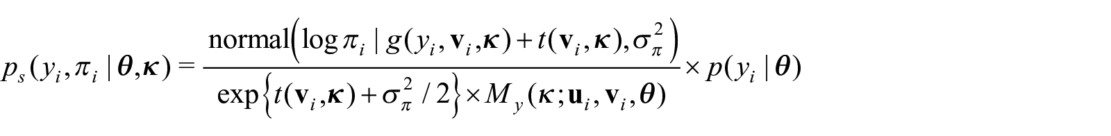
with the function $h(y_i,{\mathbf{v}}_i,\kappa )$ of the form $h(y_i,{\mathbf{v}}_i,\kappa )=g(y_i,{\mathbf{v}}_i,\kappa )+t({\mathbf{v}}_i,\kappa )$ where ${\sigma }_{\pi }^2={\sigma }_{\pi }^2(\kappa ,{\mathbf{v}}_i)$ , possibly a function of $(\kappa ,{\mathbf{v}}_i)$ then

$$p_s(y_i,{\pi }_i|\theta ,\kappa )=\frac{\mathrm{normal}\left(\log {\pi }_i|g(y_i,{\mathbf{v}}_i,\kappa )+t({\mathbf{v}}_i,\kappa ),{\sigma }_{\pi }^2\right)}{\exp \left\{t({\mathbf{v}}_i,\kappa )+{\sigma }_{\pi }^2/2\right\}\times M_y(\kappa ;{\mathbf{u}}_i,{\mathbf{v}}_i,\theta )}\times p(y_i|\theta )$$

with $M_y(\kappa ;{\mathbf{u}}_i,{\mathbf{v}}_i,\theta ):=E_{y_i^{\star }|\theta }\left[\exp \left\{g(y_i^{\star },{\mathbf{v}}_i,\kappa )\right\}\right]$ .

Theorem 1 guarantees a closed form expression for $p_s$ in Equation (2) when $p(y_i|\theta )$ and $M_y(\kappa ;\cdots )$ have closed forms. For the particular case of $g(y_i,{\mathbf{v}}_i,\kappa )={\kappa }_y{y}_i$ with ${\kappa }_y\in \Re$ an entry in $\kappa$ , $M_y$ is the moment generating function (MGF) of the population distribution of $y_i|\theta$ , evaluated at ${\kappa }_y$ . Similarly, if we wanted to include an interaction of the response and other covariate, say $v_{i\ell }$ , in the model for ${\pi }_i|y_i,\kappa$ , we may define $g(y_i,{\mathbf{v}}_i,\kappa )={\kappa }_y{y}_i+{\kappa }_{y\ell }{v}_{i\ell }{y}_i$ with ${\kappa }_y,{\kappa }_{y\ell }\in \Re$ entries of $\kappa$ , then $M_y$ is the MGF at evaluated at ${\kappa }_y+{\kappa }_{y\ell }{v}_{i\ell }$ . As discussed in LS2019, the assumption of a lognormal distribution for πi is mathematically attractive since πi, for individual $i$ , is usually calculated as the product of inclusion probabilities across the stages of the multistage survey design. If each of these stage-wise probabilities are lognormal then their product, $\propto {\pi }_i$ , is lognormal as well.

As long as $t({\mathbf{v}}_i,\kappa )={\kappa }_0+\dots$ contains an intercept term, ${\kappa }_0$ , we may assume that πi is proportional, as opposed to exactly equal, to the inclusion probability for unit $i$ . In other words, no restriction is imposed on ${\Sigma }_i{\pi }_i$ where the index $i$ could run over the population or sample indices. This is true since ${\pi }_i\sim \mathrm{lognormal}({\kappa }_0+\cdots ,\cdots )$ implies that $c\times {\pi }_i\sim \mathrm{lognormal}({\kappa }_0+\log c+\cdots ,\cdots )$ where $c>0$ is any constant and we do not make any inference on the intercept, ${\kappa }_0$ . We recommend to include the variables used for non-response or post-stratification to population totals adjustments in the vector of covariates ${\mathbf{v}}_i$ so condition (C1), introduced after Equation (4), holds for the available (estimated) πis in the sample, that is, $(y_1,{\pi }_1),\dots ,(y_n,{\pi }_n)|\theta ,\kappa$ are independent. (yi, πi)s are independent if $y_1,\dots ,y_n|\theta$ are independent and if ${\pi }_1,\dots ,{\pi }_n|y_1,\dots ,y_n,\theta ,\kappa$ are independent. The latter independence assumption follows if the relationship between the expected value of log pi and the adjustment variables is well captured by $h(y_i,{\mathbf{v}}_i,\kappa )$ . If adjustments are done, as usually, by multiplying the selection weights, $w_{sel,i}\propto 1/\mathrm{Pr}\left[\mathrm{population}\mathrm{individual}i\mathrm{being}\mathrm{invited}\mathrm{to}\mathrm{participate}\mathrm{in}\mathrm{the}\mathrm{survey}\right]$ , by non-response and/or post-stratification weights, the linear relationship between log (πi) and the adjustment variables is appropriate. For example, if nonresponse weights for Hispanics is estimated as the inverse of the response rate for Hispanics $R{R}_H$ among the individuals invited to participate in the survey, $w_i=w_{sel,i}\times 1/R{R}_H$ , $\log {\pi }_i=-\log w_i=-\log (w_{sel,i})+\log (R{R}_H)$ and ${\pi }_i\perp {\pi }_{i^{\prime }}|y_i,y_{i^{\prime }}\theta ,\kappa$ for $i^{\prime }\ne i$ conditioning on race/ethnicity (included in ${\mathbf{v}}_i$ ).

In the sequel, we adapt and extend LS2019 to our particular repeated measurements setup set of conditions in LS2019 on $p({\pi }_i|y_i,\kappa )$ under a likelihood that guarantees the availability of a closed form expression for $p_s$ . This approach assumes that the inclusion probabilities are random, as opposed to the frequentist pseudolikelihood approach discussed later in Section 4 that assumes them fixed.

3. Approach

3.1. Repeated Measures Under Informative Sampling

We consider the mixed effects linear regression population model (for repeated measures),

$$y_{im}={\mathbf{u}}_{im}^t\beta +{\delta }_i+{ϵ}_{im}\mathrm{with}{ϵ}_{im}\stackrel{\mathrm{iid}}{\sim }normal\left(0,{\sigma }_y^2\right)\mathrm{and}{\delta }_i\stackrel{\mathrm{iid}}{\sim }normal\left(0,{\sigma }_{\delta }^2\right),$$

(5)

for each individual $i$ in the population, and $m=1,\dots ,M_i$ , the total number of repeated measures for individual, $i$ . Here, the double index $im$ indexes the population individual $i$ at measurement occasion $m$ ; $y_{im}$ is associated value for the response variable; ${\mathbf{u}}_{im}$ is a $q_y$ dimension vector of covariates whose first entry is set equal to 1 so the model includes an intercept coefficient; and, ${\delta }_i$ is a participant-specific random effect (P-RE).

Denote with ${\mathbf{y}}_i=(y_{i1},y_{i2},\dots ,y_{i,M_i}{)}^t$ the vector of all measurements for individual $i$ and ${\mathbf{u}}_i=(ui1qy\times 1;...;uiMi)$ the $q_y\times M_i$ matrix whose column $m$ corresponds to covariates at occasion $m$ for individual $i$ . In applications, usually multiple entries of ${\mathbf{u}}_{im}$ and ${\mathbf{u}}_{i{m}^{\prime }}$ naturally match or are exactly equal; for example, when the entry $\ell$ of ${\mathbf{u}}_{im}$ , $u_{im,\ell }$ , encodes the participant’s gender or baseline weight, $u_{im,\ell }=u_{i{m}^{\prime },\ell }$ . The population model in Equation (5) is equivalent to

$${\mathbf{y}}_i\sim MV{N}_{M_i}\left({\mathbf{u}}_i^t\beta ,{\Sigma }_{M_i}\right),\mathrm{for}\mathrm{individual}i\mathrm{in}\mathrm{the}\mathrm{population}$$

(6)

with ${\Sigma }_{M_i}={\sigma }_y^2{I}_{M_i}+{\sigma }_{\delta }^2{\mathbf{1}}_{M_i}{\mathbf{1}}_{M_i}^t$ . We parameterize an equal correlation structure but other structures, for example, first order autoregressive, may also be used.

Following LS2019, our Bayesian approach accounts for the informative sampling design by modeling the joint distribution of (yi, pi), $p({\mathbf{y}}_i,{\pi }_i|\theta ,\kappa )=p({\mathbf{y}}_i|\theta )p({\pi }_i|{\mathbf{y}}_i,\kappa )$ , where $p({\mathbf{y}}_i|\theta )$ is the PDF of the distribution in Equation (6) with $\theta :=(\beta ,{\sigma }_{\delta },{\sigma }_y)$ ; and $p({\pi }_i|{\mathbf{y}}_i,\kappa )$ is discussed below.

Similar to the set of covariates for ${\mathbf{y}}_i$ , we denote with qp the number of covariates used to model ${\pi }_i|{\mathbf{y}}_i,\kappa$ ; and, ${\mathbf{v}}_{im}$ the qp dimensional vector of these covariate values for individual $i$ at occasion $m$ . The first entry of ${\mathbf{v}}_{im}$ is set equal to 1 to include an intercept and it is common that $v_{im,\ell }=v_{i{m}^{\prime },\ell }$ , where $v_{im,\ell }$ is the entry $\ell$ of ${\mathbf{v}}_{im}$ . We denote with ${\mathbf{v}}_i=(vi1q\pi \times 1;...;vi,Mi)$ the $q_{\pi }\times M_i$ matrix of covariates. Note that we allow for ${\mathbf{v}}_{im}$ and ${\mathbf{u}}_{im}$ to have common covariates or even being equal. For example gender can be used to model both with ${\mathbf{y}}_i|\theta$ and ${\pi }_i|{\mathbf{y}}_i,\kappa$ . Also note that the distributions of ${\mathbf{y}}_i|\theta$ and ${\pi }_i|{\mathbf{y}}_i,\kappa$ depend, implicitly, on the quantities ${\mathbf{u}}_i$ and ${\mathbf{v}}_i$ , respectively, but, since they are fixed quantities and to ease notation, we will omit them from the notation of the conditional distributions.

Theorem 2 below presents an extension of Theorem 1 adapted to the repeated measures formulation of Equation (6). The vectors ${\mathbf{y}}_i$ and $\theta$ in Theorem 2 play the role, respectively, of the univariate response $y_i$ and $\theta$ in Theorem 1. Note that in Theorem 2, we work with the model in Equation (6), where the participant-specific random effects, ${\delta }_i$ , is marginalized to later bring it back in Equation (11).

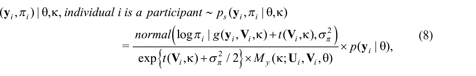
• Theorem 2. If the population distribution of ${\pi }_i|{\mathbf{y}}_i,\kappa$ is

$${\pi }_i|{\mathbf{y}}_i,\kappa \sim lognormal\left(h\left({\mathbf{y}}_i,{\mathbf{v}}_i,\kappa \right),{\sigma }_{\pi }^2\right)$$

(7)

with the function $h({\mathbf{y}}_i,{\mathbf{v}}_i,\kappa )$ of the form $h({\mathbf{y}}_i,{\mathbf{v}}_i,\kappa )=g({\mathbf{y}}_i,{\mathbf{v}}_i,\kappa )+t({\mathbf{v}}_i,\kappa )$ where ${\sigma }_{\pi }^2={\sigma }_{\pi }^2({\mathbf{v}}_i,\mathrm{k})$ , possibly a function of $({\mathbf{v}}_i,\kappa )$ then the exact likelihood for the observed sample takes the form,

$$\begin{array}{l}({\mathbf{y}}_i,{\pi }_i)|\theta ,\kappa ,individualiisaparticipant\sim p_s({\mathbf{y}}_i,{\pi }_i|\theta ,\kappa )\\ =\frac{normal\left(\log {\pi }_i|g({\mathbf{y}}_i,{\mathbf{v}}_i,\kappa )+t({\mathbf{v}}_i,\kappa ),{\sigma }_{\pi }^2\right)}{\exp \left\{t({\mathbf{v}}_i,\kappa )+{\sigma }_{\pi }^2/2\right\}\times M_y(\kappa ;{\mathbf{u}}_i,{\mathbf{v}}_i,\theta )}\times p({\mathbf{y}}_i|\theta ),\end{array}$$

(8)

with $M_y(\kappa ;{\mathbf{u}}_i,{\mathbf{v}}_i,\theta ):=E_{{\mathbf{y}}_i^{\star }|\theta }\left[\exp \left\{g({\mathbf{y}}_i^{\star },{\mathbf{v}}_i,\kappa )\right\}\right]$ .

Recall that use the superindex ⋆ to denote the quantity being integrated out. We next discuss a common model setting that yields a closed form for Equation (8). If we choose $g({\mathbf{y}}_i,{\mathbf{v}}_i,\kappa ):={\kappa }_y{\overline{y}}_{i\cdot }$ with ${\overline{y}}_{i\cdot }=(1/M_i){\Sigma }_{m=1}^{M_i}{y}_{im}$ the average of the repeated measures of individual $i$ ; and, ${\kappa }_y$ depending on $\kappa$ and, perhaps, on ${\mathbf{v}}_i$ , then,

$$M_y(\kappa ;{\mathbf{u}}_i,{\mathbf{v}}_i,\theta ):=E_{{\mathbf{y}}_i^{\star }|\theta }\left[\exp \left({\kappa }_y{\overline{y}}_{i\cdot }^{\star }\right)\right]$$

is the MGF of ${\overline{y}}_{i\cdot }^{\star }$ evaluated at ${\kappa }_y$ . Under the population model in Equation (6), ${\overline{y}}_{i\cdot }^{\star }\sim normal\left({\overline{\mathbf{u}}}_{i\cdot }^t\beta ,{\sigma }_y^2/M_i+{\sigma }_{\delta }^2\right)$ with ${\overline{\mathbf{u}}}_{i\cdot }={\Sigma }_{m=1}^{M_i}{\mathbf{u}}_{im}/M_i$ , a column vector of dimension $q_y$ . Since the $\mathrm{normal}(m,s^2)$ distribution has $\mathrm{MGF}(t)=\exp [tm+t^2{s}^2/2]$ , $M_y(\kappa ;{\mathbf{u}}_i,{\mathbf{v}}_i,\theta )=\exp \left[{\kappa }_y{\overline{\mathbf{u}}}_{i\cdot }^t\beta +{\kappa }_y^2\left({\sigma }_y^2/M_i+{\sigma }_{\delta }^2\right)/2\right]$ , defining $t({\mathbf{v}}_i,\mathrm{k})={\overline{\mathbf{v}}}_{i\cdot }^t{\mathrm{k}}_{\mathbf{v}}$ with ${\overline{\mathbf{v}}}_{i\cdot }={\Sigma }_{m=1}^{M_i}{\mathbf{v}}_{im}/M_i$ , a qp-dimensional vector, Equation (7) becomes

$${\pi }_i|{\mathbf{y}}_i,\kappa \sim lognormal({\kappa }_y{\overline{y}}_{i\cdot }+{\overline{\mathbf{v}}}_{i\cdot }^t{\kappa }_{\mathbf{v}},{\sigma }_{\pi }^2)$$

(9)

and Equation (8) becomes

$$\begin{array}{l}\begin{array}{l}{p}_s({\mathbf{y}}_i,{\pi }_i|\theta ,\kappa )=\left\{\frac{\mathrm{normal}\left(\log {\pi }_i|{\kappa }_y{\overline{y}}_{i\cdot }+{\overline{\mathbf{v}}}_{i\cdot }^t{\kappa }_{\mathbf{v}},{\sigma }_{\pi }^2\right)}{\exp \left[{\overline{\mathbf{v}}}_{i\cdot }^t{\kappa }_{\mathbf{v}}+{\sigma }_{\pi }^2/2\right]\times \exp \left[{\kappa }_y{\overline{\mathbf{u}}}_{i\cdot }^t\beta +{\kappa }_y^2\left({\sigma }_y^2/M_i+{\sigma }_{\delta }^2\right)/2\right]}\right\}\\ \times MV{N}_{M_i}({\mathbf{y}}_i|{\mathbf{u}}_i^t\beta ,{\Sigma }_{M_i})\end{array}\hfill \end{array}$$

(10)

with $\kappa =\left({\kappa }_y,{\kappa }_{\mathbf{v}},{\sigma }_{\pi }\right)$ and $\theta =\left(\beta ,{\sigma }_y,{\sigma }_{\delta }\right)$ . Recall that both $\beta$ and ${\kappa }_{\mathbf{v}}$ include and intercept coefficient. Notice that we could have also used $g\left({\mathbf{y}}_i,{\mathbf{v}}_i,\kappa \right):={\Sigma }_m{\kappa }_{ym}{y}_{im}$ or $t({\mathbf{v}}_i,\kappa )={\Sigma }_m{\mathbf{v}}_{im}^t{\kappa }_{\mathbf{v}m}$ to give different weights to each repeated measure (response and covariates, respectively) in the distribution of $\log {\pi }_i|{\mathbf{y}}_i,\kappa$ . Similar arguments as the one to derive Equation (10) would give us a close form for $p_s$ in Equation (8).

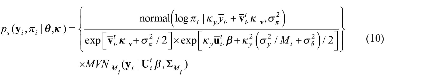
For ease-of-conducting our simulation study we opt to retain and not marginalize over the participant-specific random effect, treating it as latent variable as an entirely equivalent specification as Equation (10) to obtain,

$$p_s({\mathbf{y}}_i,{\pi }_i|\theta ,{\delta }_i,\kappa )=\{\cdots \}{\Pi }_{m=1}^{M_i}normal(y_{im}|{\mathbf{u}}_{im}^t\beta +{\delta }_i,{\sigma }_y^2)\mathrm{with}{\delta }_i|\theta \stackrel{\mathrm{iid}}{\sim }normal(0,{\sigma }_{\delta }^2)$$

(11)

with {⋯} the quantity within curly brackets in Equation (10). The likelihood under $y_i|\theta ,{\delta }_i$ given in Equation (5) is

$$Like\left(\theta ,({\delta }_1,\dots ,{\delta }_n),\kappa ;({\mathbf{y}}_1,{\pi }_1),\dots ,({\mathbf{y}}_n,{\pi }_n)\right)\propto {\Pi }_{i=1}^n{p}_s({\mathbf{y}}_i,{\pi }_i|\theta ,{\delta }_i,\kappa )$$

(12)

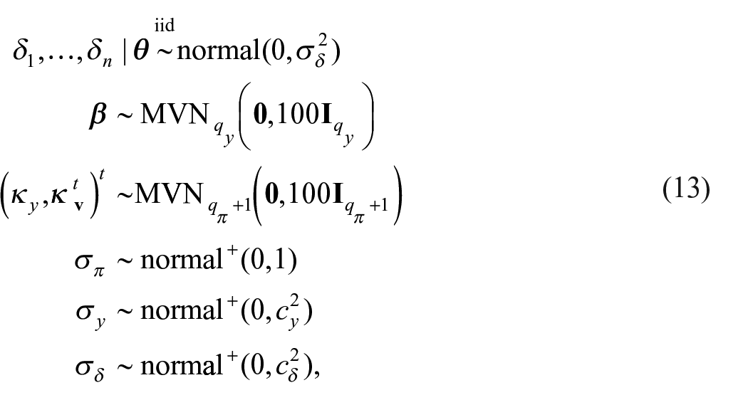
The sample size is $n$ and without loss of generality $i=1,\dots ,n$ now indexes the participants (in the observed sample), as opposed to the individual in the population. The expression in Equation (11) represents an augmented likelihood for $(y_{im},{\delta }_i)$ and constructs an augmented posterior distribution when combined with prior distributions for the model global parameters (e.g., $(\beta ,\kappa ,{\sigma }_{\pi },{\sigma }_y)$ ). The parameter inducing the dependence between ${\mathbf{y}}_i$ and πi is ${\kappa }_y$ ; and, ${\mathbf{y}}_i\perp {\pi }_i|{\kappa }_y=0$ . A 95% credible interval of ${\kappa }_y$ non containing zero indicates that the sampling design is informative for the response $\mathbf{y}$ . For details on how to define Equation (11) and (12) in Stan code see appendix subsection A.4. In our set-up, since ${\delta }_i$ is latent, we estimate it using the prior distribution ${\delta }_1,\dots ,{\delta }_n|\theta \stackrel{\mathrm{iid}}{\sim }normal(0,{\sigma }_{\delta }^2)$ starting with Equation (12). We then proceed to select priors for $\theta$ and $\kappa$ to complete the specification of the Bayesian model. We choose the following priors:

$$\begin{array}{c}{\delta }_1,\dots ,{\delta }_n|\theta \stackrel{\mathrm{iid}}{\sim }normal(0,{\sigma }_{\delta }^2)\\ \beta \sim MV{N}_{q_y}\left(\mathbf{0},100{\mathbf{I}}_{q_y}\right)\\ {\left({\kappa }_y,{\kappa }_{\mathbf{v}}^t\right)}^t\sim {\mathrm{MVN}}_{q_{\pi }+1}\left(\mathbf{0},100{\mathbf{I}}_{q_{\pi }+1}\right)\\ {\sigma }_{\pi }\sim norma{l}^{+}(0,1)\\ {\sigma }_y\sim norma{l}^{+}(0,c_y^2)\\ {\sigma }_{\delta }\sim norma{l}^{+}(0,c_{\delta }^2),\end{array}$$

(13)

where the priors on the global parameters are chosen to be vague or weakly informative. Here $norma{l}^{+}(\mu ,{\sigma }^2)$ denotes the $normal(\mu ,{\sigma }^2)$ distribution restricted to the positive real line. When implementing, we standardize the inclusion probabilities so that ${\Sigma }_{i=1}^{n}1/{\pi }_i={\Sigma }_i{M}_i$ , the total number of measurements, matching the standardization of the pseudolikelihood approach below (Section 4). This way the πis are neither too small nor too large so that the prior distribution for ${\sigma }_{\pi }$ in Equation (13) is vague. The hyperparameters $c_y^2$ and $c_{\delta }^2$ are chosen large enough so the priors are vague. For example, $c_y^2$ is chosen to be larger than the average over $m$ of the sample variances of $\left\{y_{im}\right|i=1,\dots ,n\}$ and $c_{\delta }^2$ is chosen to be larger than the sample covariance of $\{(y_{i1},y_{i2}),i=1,\dots ,n\}$ . In the next subsection we extend the proposed method to incorporate primary sampling unit information into the statistical analysis based on León-Novelo and Savitsky (2023). If not of interest this subsection may be skipped.

3.2. Including PSU Information into the Analysis

NHANES data are collected through a complex sampling design. First the U.S. is divided into fifteen strata and two primary sampling units (PSUs) are sampled within each stratum. Strata are defined by the intersection of geography with concentrations of minority populations and a PSU is constructed as a county or a group of geographically contiguous counties. The NHANES data are packaged with variables of interest for each survey participant along with the stratum and PSU identifiers to which s/he belongs to as well as sampling weights. NHANES releases masked stratum and PSU information to protect participant’s privacy. Every two-year NHANES-data cycle (CDC 2011) releases information obtained from $H=15$ strata with $n_h=2$ PSU per stratum.

León-Novelo and Savitsky (2023) incorporate PSU information into the analysis to account for both possible correlations among the responses of individuals in the same PSU and for informative sampling with respect to PSU (i.e., when the probability of sampling the PSU is not independent of the values of the response variable for nested units). Their approach consists of including a PSU-specific RE (PSU-RE) in both the model for the response and the inclusion probability. They show that the inclusion of these random effects produce correct uncertainty quantification, that is, $1-\alpha$ credible intervals with $1-\alpha$ coverage. León-Novelo and Savitsky (2023) do not consider repeated measures. We now further extend the PSU-REs formulation in León-Novelo and Savitsky (2023) to the repeated measures model in Subsection 3.1. This extension includes a participant-specific RE in the model for the response, and PSU-REs in the models for the response and the inclusion probability.

Let $J$ denote the number of PSUs in the sample where $j=1,\dots ,J$ denotes the PSU index and $n_j$ denotes the number of observations nested in PSU $j$ . We retain the notation from previous sections replacing the subindex, $i$ with $ij$ , where now the index $i$ runs from $1,\dots ,n_j$ ; $M_{ij}$ now denotes the number of occasions the response was measured for individual $i$ in PSU $j$ ; ${\mathbf{y}}_{ij}$ , πij, and ${\mathbf{u}}_{ij}=({\mathbf{u}}_{ij1};\dots ;{\mathbf{u}}_{ij{M}_{ij}})$ denote, respectively, the $M_{ij}$ dimensional vector of repeated response measures, the inclusion probability of individual $ij$ as a participant, and the $q_y\times M_{ij}$ matrix with $m^{th}$ column, ${\mathbf{u}}_{ij}$ , the vector of covariates at occasion $m$ , for the participant $i$ in the PSU $j$ . The first entry of ${\mathbf{u}}_{ijm}$ , $m=1,\dots ,M_{ij}$ is set to 1 so the model includes an intercept. Adding the PSU-RE, ${\eta }_j$ , to the model in Equation (6) yields,

$${\mathbf{y}}_{ij}|\theta ,\eta \sim MV{N}_{M_{ij}}\left({\mathbf{u}}_{ij}^t\beta +{\eta }_j{\mathbf{1}}_{M_{ij}},{\Sigma }_{M_{ij}}\right)\mathrm{for}i=1,\dots ,n_j\mathrm{and}j=1,\dots ,J$$

(14)

with ${\Sigma }_{M_{ij}}={\sigma }_y^2{\mathrm{I}}_{M_{ij}}+{\sigma }_{\delta }^2{\mathbf{1}}_{M_{ij}}{\mathbf{1}}_{M_{ij}}^t$ ; $\theta =\left(\beta ,{\sigma }_y,{\sigma }_{\delta }\right)$ ; and ${\eta }_1,\dots ,{\eta }_J\stackrel{\mathrm{iid}}{\sim }normal\left(0,{\sigma }_{\eta }^2\right)$ .

Adding the PSU-RE, ${\eta }_j^{\pi }$ , in the model for πi defined in Equation (9) yields,

$${\pi }_{ij}|{\mathbf{y}}_{ij},\kappa ,{\eta }_j^{\pi }\sim lognormal\left({\kappa }_y{\overline{y}}_{ij\cdot }+{\overline{\mathbf{v}}}_{ij\cdot }^t{\kappa }_{\mathbf{v}}+{\eta }_j^{\pi },{\sigma }_{\pi }^2\right),\mathrm{for}i=1,\dots ,n_j\mathrm{and}j=1,\dots ,J$$

(15)

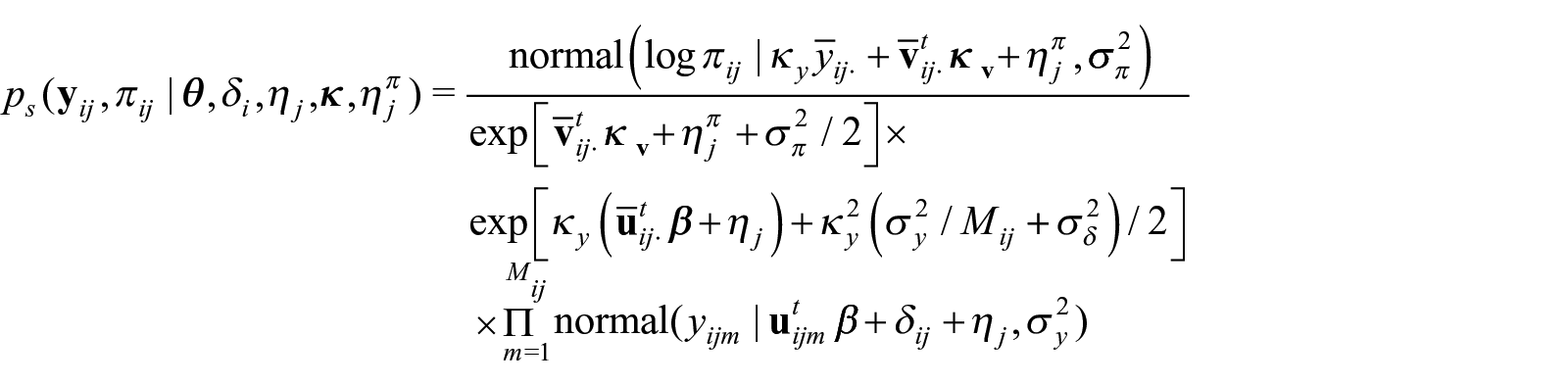
with $\kappa =\left({\kappa }_y,{\kappa }_{\mathbf{v}},{\sigma }_{\pi }^2\right)$ ; ${\eta }_1^{\pi },\dots ,{\eta }_J^{\pi }\stackrel{\mathrm{iid}}{\sim }normal\left(0,{\sigma }_{{\eta }^{\pi }}^2\right)$ ; ${\overline{y}}_{ij\cdot }=(1/M_{ij}){\Sigma }_{m=1}^{M_{ij}}{y}_{ijm}$ and ${\overline{\mathbf{v}}}_{ij\cdot }=(1/M_{ij})\Sigma {\mathbf{v}}_{ijm}$ and ${\mathbf{v}}_{ijm}$ the vector of covariate at measurement occasion $m$ used to model ${\pi }_{ij}|{\mathbf{y}}_{ij},\kappa ,{\eta }_j^{\pi }$ . So, reintroducing the P-RE, ${\delta }_{ij}$ , the analogous to Equation (11) is (this is, just replacing ${\overline{\mathbf{v}}}_{i\cdot }^t{\kappa }_{\mathbf{v}}\to {\overline{\mathbf{v}}}_{ij\cdot }^t{\kappa }_{\mathbf{v}}+{\eta }_j^{\pi }$ ; and, ${\mathbf{u}}_{im}^t\beta \to {\mathbf{u}}_{ijm}^t\beta +{\eta }_j$ in Equation (11)).

$$\begin{array}{l}\begin{array}{l}{p}_s({\mathbf{y}}_{ij},{\pi }_{ij}|\theta ,{\delta }_i,{\eta }_j,\kappa ,{\eta }_j^{\pi })=\frac{normal\left(\log {\pi }_{ij}|{\kappa }_y{\overline{y}}_{ij\cdot }+{\overline{\mathbf{v}}}_{ij\cdot }^t{\kappa }_{\mathbf{v}}+{\eta }_j^{\pi },{\sigma }_{\pi }^2\right)}{\begin{array}{l}\exp \left[{\overline{\mathbf{v}}}_{ij\cdot }^t{\kappa }_{\mathbf{v}}+{\eta }_j^{\pi }+{\sigma }_{\pi }^2/2\right]\times \\ \exp \left[{\kappa }_y\left({\overline{\mathbf{u}}}_{ij\cdot }^t\beta +{\eta }_j\right)+{\kappa }_y^2\left({\sigma }_y^2/M_{ij}+{\sigma }_{\delta }^2\right)/2\right]\end{array}}\\ \times {\Pi }_{m=1}^{M_{ij}}normal(y_{ijm}|{\mathbf{u}}_{ijm}^t\beta +{\delta }_{ij}+{\eta }_j,{\sigma }_y^2)\end{array}\hfill \end{array}$$

with now ${\delta }_{1,1},\dots ,{\delta }_{n_1,1},{\delta }_{1,2},\dots ,{\delta }_{n_2,2},\dots ,{\delta }_{1J},\dots ,{\delta }_{n_J,J}\stackrel{\mathrm{iid}}{\sim }N(0,{\sigma }_{\delta }^2)$ . Since the qualities of this approach have been reported in León-Novelo and Savitsky (2023), we will not consider it in our simulation section. This model will be fit in the application section with the priors defined in Equation (13) and ${\sigma }_{{\eta }^{\pi }},{\sigma }_{\eta }\stackrel{\mathrm{iid}}{\sim }norma{l}^{+}(0,1)$ .

4. Pseudolikelihood

Savitsky and Williams (2019) (see their Theorem 2) propose an approach to incorporate sampling weights and random effects using a plug-in augmented pseudolikelihood that for the repeated measures set-up of Subsection 3.1 is:

$${\Pi }_{i=1}^n\left\{\left[{\Pi }_{m=1}^{M_i}p{(y_{im}|\theta )}^{w_i}\right]\times p{\left({\delta }_i|{\sigma }_{\delta }^2\right)}^{w_i}\right\}$$

(16)

with the sampling weights standardized so ${\Sigma }_{i=1}^n{M}_i{w}_i={\Sigma }_{i=1}^n{M}_i$ . In Subsection A.3 we present the original formula in Theorem 2 of Savitsky and Williams (2019) and derive (16) as a specific case of this formula. The contribution of the observation for a unit, $y_{im}$ , to the pseudolikelihood is its PDF (or what it would contribute to the likelihood) exponentiated to its sampling weight, $w_i$ . The prior distribution for the random effects is also exponentiated by sampling weights, $w_i$ . The sampling weights, $w_i$ are standardized so they sum the number of participant/occasion observations. For example if we have 100 participants with two observations the standardized sampling weights must sum $100\times 2=200$ , that is, ${\Sigma }_{i=1}^n{w}_i=200$ .

The observed data pseudolikelihood for $y_{im}$ together with the pseudo prior for the random effects, ${\delta }_i$ , formulate an augmented data likelihood. The participant-specific random effects are used to account for dependence among the repeated measures. Since ${[normal(x|\mu ,{\sigma }^2)]}^w\propto normal(x|\mu ,{\sigma }^2/w)$ the pseudolikelihood approach in linear regression is equivalent to the regression model:

$$y_{im}={\mathbf{u}}_{im}^t\beta +{\delta }_i+{ϵ}_{im}\mathrm{with}{ϵ}_{im}\sim normal\left(0,{\sigma }_y^2/w_i\right)$$

with ${\delta }_i\sim normal\left(0,{\sigma }_{\delta }^2/w_i\right)$ , for $m=1,\dots ,M_i$ and $i=1,\dots ,n$ .

The advantages of the pseudolikelihood approach over the proposed fully Bayesian approach are: (A) It incorporates weights into the power term of the likelihood function so that relatively little modifications are performed to the population model sampler to incorporate the pseudo likelihood; (B) Specification of πi $|y_i,\cdots$ for the population is not necessary; (C) There is no expected value

$$\mathrm{Pr}\left(\mathrm{individual}i\mathrm{becomes}\mathrm{a}\mathrm{participant}|\theta ,\kappa \right)=E_{y_i^{\star }|\theta }\left[E({\pi }_i^{\star }|y_i^{\star },\kappa )\right]$$

(the denominator in Equation 2 to compute as in the fully Bayes method. Note than in (C), the inner and outer expectations may depend in a set of covariates ${\mathbf{v}}_i$ and ${\mathbf{u}}_i$ , respectively.

The disadvantages of the pseudo posterior approach are: (A) It is not fully Bayesian; (B) The sampling weights are only needed for unbiased estimation to the extent that they are dependent on the response variable of interest. Any variation in the weights not related to the response variable represents noise. The pseudo posterior distribution does not discard variation in weights that is independent of the response variable, so information unrelated to the response introduces noise into the estimation of the pseudo posterior distribution; (C) The weights must be normalized to regulate the amount of estimated posterior uncertainty, which is not required for the fully Bayes approach (except to specify a vague prior for πi as discussed after equation 13); and, (D) The sampling weights are inversely proportional to the inclusion probabilities. The inclusion probabilities represent a distribution that governs the taking of samples from the population that we call the “sampling design” distribution. The resulting credible intervals of the pseudolikelihood do not account for uncertainty with respect to the sampling design distribution because they treat the inclusion probabilities as fixed.

The pseudolikelihood is used here because it is convenient in that the Bayesian data analyst may use the same model and posterior sampling algorithm as defined for the population and only exponentiates the likelihood contributions by the associated sampling weights. While the pseudoposterior is not our recommended (fully Bayesian) method because it is known that it produces incorrect credible intervals, we include it as a comparison to our fully Bayes procedure because it is the commonly used method in practice due to its ease of implementation.

We implement the pseudolikelihood approach in the sequel as a Bayesian version of the NCI method. The pseudolikelihood approach uses one-step estimation, instead of the two-step estimation algorithm of the NCI approach, which propagates uncertainty in estimation of parameters, but is otherwise equivalent. We show that the fully Bayes approach outperforms the pseudolikelihood approach in terms of bias, MSE, and 95% of CI coverage.

5. Simulation Study

We perform a Monte Carlo simulation study to compare the performance of our fully Bayes method in Subsection 3.1 with the pseudolikelihood approach in Section 4. In each Monte Carlo iteration, we generate a population of size $N_{pop}{=10}^5$ . The information constructed for each individual in the population is its inclusion probability, two repeated measures, and the value of a predictor at each measurement occasion. Next, we generate an informative sample and a simple random sample. The former is analyzed with our fully Bayes method, the pseudolikelihood approach and the model in Equation (5) that ignores the informativeness of the sample (labeled POP). The simple random sample is analyzed with the model (5) (label this analysis SRS). The SRS is included to serve as a benchmark for point estimation and uncertainty quantification and is compared to methods estimated on the informative sample taken from the same population. For each population and sample we apply the estimation approaches of our fully Bayes method and associated comparator methods, assessing the bias, MSE, and coverage properties. We focus on inference about ${\beta }_0$ as a global parameter of inferential interest. We will repeat steps 1 to 3 below $M=1000$ (say) times:

1. Generate a population of $N_{pop}{=10}^5$ individuals. For $i=1,\dots ,N_{pop}$ , generate:

2. (b) predictors $u_{i1},u_{i2}\stackrel{\mathrm{iid}}{\sim }normal\left(0,1\right)$ ;

3. (c) individual-specific random effects ${\gamma }_i\stackrel{\mathrm{iid}}{\sim }normal\left(0,{\sigma }_{\gamma }^2{=0.3}^2\right)$ ;

4. (d) response $y_{im}\sim normal\left({\mu }_{im}{,0.5}^2\right)$ with mean ${\mu }_{i1}=1-0.5u_{i1}+{\gamma }_i+{\pi }_i$ and ${\mu }_{i2}\ne 1-0.5u_{i2}+{\gamma }_i+{\pi }_i$ . Notice that the covariate values are different, $u_{i1}\ne u_{i2}$ , but the effect on the response is the same. We are adding πi to the mean so $y_i\cancel{\perp }{\pi }_i|(u_{i1},u_{i2})$ .

Generate a simple random sample (SRS) and an informative sample (IS) (without replacement), each of size $n=100$ . The IS contains $(y_{i1},y_{i2},u_{i1},u_{i2},{\pi }_i$ ) with probability ${\pi }_i/{\Sigma }_{i^{\prime }=1}^{N_{pop}}{\pi }_{i^{\prime }}$ , while the SRS uses equal probabilities of value, $1/N_{pop}$ . Note that the sum of the πis in the sample (i.e., ${\Sigma }_{i=1}^n{\pi }_i^{(s)}$ ) or in the population (i.e., ${\Sigma }_{i=1}^{N_{pop}}{\pi }_i$ ) is not standardized. Large values of $y_{i1}$ and $y_{i2}$ are more likely to be sampled (large value of πi is associated with large value of $y_{im}$ ). The simulation true parameter value of ${\beta }_0$ , the intercept, under our regression model in Equation (5) is ${\beta }_0^{Ana,TRUE}:=E(y_{im}|u_{i1}=u_{i2}=0)=1+E({\pi }_i)=1+4/2=3$ .

Analyze IS with three methods, and also the SRS. All of them assume the analysis model in Equation (5) with $\beta =({\beta }_0,{\beta }_1{)}^t$ , ${\mathbf{u}}_{im}^t=(1,u_{im})$ , and priors specified in Equation (13) with $c_y^2=c_{\delta }^2=1$ .

(a) FULL: The proposed Bayesian model in Subsection 3.1; with ${\mathbf{v}}_{im}={\mathbf{u}}_{im}$ so ${\overline{\mathbf{v}}}_i^t:=(1,(u_{i1}+u_{i2})/2)$ in Equation (15).

(b) PSEUDO: Pseudolikelihood approach as described in Section 4, with $w_i\propto 1/{\pi }_i$ .

(c) POP: Bayesian model in Equation (5), ignoring the pis.

Analyze the SRS with model (5), label this SRS analysis.

Compute and store for each one of the three models plus the analysis of the SRS:

● Point estimate of ${\beta }_0$ equal to the posterior expected value of ${\beta }_0$ .

● Central 95% CI for ${\beta }_0$ .

The above simulation study design will tend to allow non-informative inference (that allows unbiased estimation using the uncorrected population model (i.e., POP) for the slope parameter of interest, ${\beta }_1$ , for a sufficiently large sample size due to the conditioning on πi (in mi) used to generate $y_i$ . We could have added an interaction term ${\pi }_i\times u_{i1}$ in mi1 and ${\pi }_i\times u_{i2}$ in mi2 to bias the estimation of ${\beta }_1$ under the uncorrected model (POP) and require our fully Bayes likelihood for the observed sample of Equation (12) (i.e., FULL) for correct inference. For ease-of-understanding, however, we achieve the same benefit by focusing on the global intercept, ${\beta }_0$ , which is informatively estimated under the sample design.

For each method, we end up with $M$ point estimates of ${\beta }_0$ and central 95% credible intervals. Call ${\tilde{\beta }}_0^m$ , $m=1,\dots ,M$ this point estimate. Similarly call the credible interval $(L_0^m,U_0^m)$ . Estimate,

• $Bias=averag{e}_{\left\{m=1,...,M\right\}}\left\{{\tilde{\beta }}_0^m-{\beta }_0^{Ana,TRUE}\right\}$ ;

• $MSE=averag{e}_m\left\{{\left[{\tilde{\beta }}_0^m-{\beta }_0^{Ana,TRUE}\right]}^2\right\}$ ;

• Coverage = Proportion of times that the central 95% credible intervals contained ${\beta }_0^{Ana,TRUE}$ ;

• Expected length of central 95% credible intervals =  $averag{e}_m\{U_0^m-L_0^m\}$ .

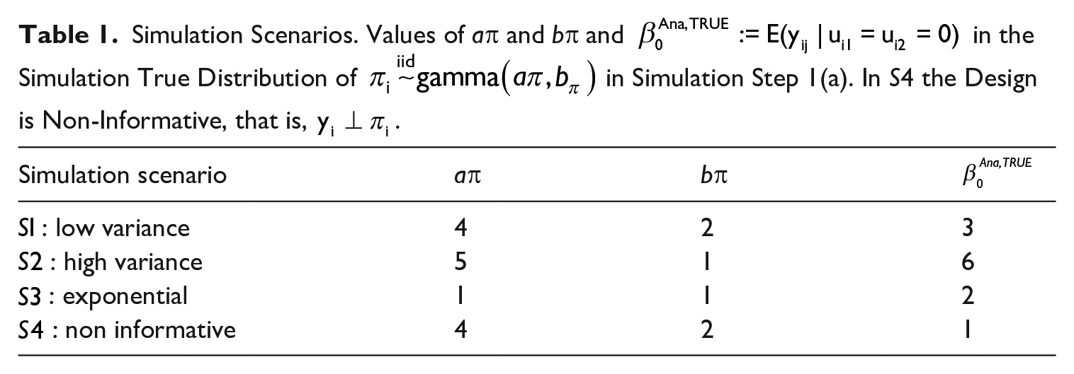
We extend the simulation to more scenarios by varying the values of of aπ and bπ in step 1(a). The values are given in Table 1. Simulation scenario $S1$ explores the performance of the methods when variance of the inclusion probabilities $\left(a_{\pi }/b_{\pi }^2=1\right)$ is low; $S2$ when it is high; $S3$ when the distribution of πi has mode 0, and thus is very different from the lognormal distribution assumed by Full in Equation (9). $S4$ is different from the three other scenarios; here we set ${\mu }_{im}=1-0.5x_{im}+{\gamma }_i$ (excluding πi) in simulation step 1(d) so the IS generated in step 2 is, actually, non-informative such that sampling weights are not needed to correct the sample model. $S4$ explores the performance of the methods design to analyze informative samples when the design is actually non-informative, and thus the weights, $\propto 1/{\pi }_i$ are noise.

Table 1.

Simulation Scenarios. Values of ap and bp and ${\beta }_0^{Ana,TRUE}:=E(y_{ij}|u_{i1}=u_{i2}=0)$ in the Simulation True Distribution of ${\pi }_i\stackrel{iid}{\sim }gamma\left(a\pi ,b_{\pi }\right)$ in Simulation Step 1(a). In S4 the Design is Non-Informative, that is, $y_i\perp {\pi }_i$ .

Simulation scenario	$a_{\pi }$ ap	$b_{\pi }$ bp	${\beta }_0^{Ana,TRUE}$
$S1$ : low variance	4	2	3
$S2$ : high variance	5	1	6
$S3$ : exponential	1	1	2
$S4$ : non informative	4	2	1

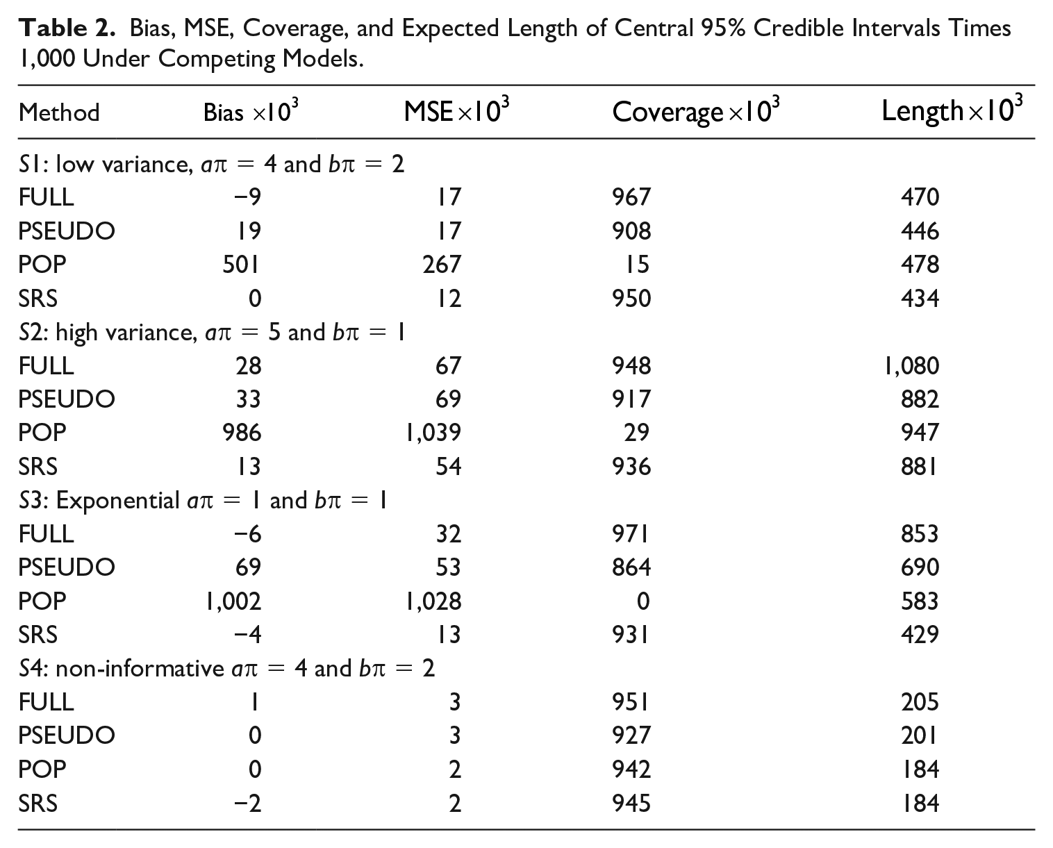
Table 2 shows the results. FULL and PSEUDO yield similar point inference quality (i.e., similar bias and MSE) but only FULL yields appropriate uncertainty quantification (i.e., CI reaching nominal coverage). In $S1-S3$ , FULL and PSEUDO perform similar in terms of bias and MSE, but the PSEUDO central 95% CIs undercover because this approach does not account for the uncertainty induced by the sampling design distribution. The FULL CIs coverage is similar to that for the benchmark SRS at the cost of being wider than SRS CIs. The sampling design can produce estimators that are more or less efficient, depending on the construction for inclusion probabilities. In general, the use of strata makes the sampling design more efficient than SRS, but clustering into PSUs (which is done for convenience of survey administration) is less efficient; meaning, that it produces longer credible intervals. In $S1-S3$ , POP yields, as expected, biased inference, showing the consequences of not adjusting inference for informative design. These scenarios, but particularly $S3$ where the simulation true exponential distribution of πi has mode at zero (while the density of any lognomal distribution evaluated at zero equals zero), show that FULL is robust against the violation of the lognormal distribution of the πis that is assumed in Equation (9). $S4$ shows that FULL and PSEUDO coverage is appropriate even when the sample is non informative.

Table 2.

Bias, MSE, Coverage, and Expected Length of Central 95% Credible Intervals Times 1,000 Under Competing Models.

Method	$Bias\times 10^3$	$MSE\times 10^3$	$Coverage\times 10^3$	$Length\times 10^3$
$\mathcal{S}1$ S1: low variance, aπ = 4 and bπ = 2
FULL	−9	17	967	470
PSEUDO	19	17	908	446
POP	501	267	15	478
SRS	0	12	950	434
$\mathcal{S}2$ : high variance, aπ = 5 and bπ = 1
FULL	28	67	948	1,080
PSEUDO	33	69	917	882
POP	986	1,039	29	947
SRS	13	54	936	881
$\mathcal{S}3$ : Exponential aπ = 1 and bπ = 1
FULL	−6	32	971	853
PSEUDO	69	53	864	690
POP	1,002	1,028	0	583
SRS	−4	13	931	429
$\mathcal{S}4$ : non-informative aπ = 4 and bπ = 2
FULL	1	3	951	205
PSEUDO	0	3	927	201
POP	0	2	942	184
SRS	−2	2	945	184

As a side note, the data generating model in step 1, generates first the inclusion probability p (in 1.a) and then ${\mathbf{y}}_i|$ πi in (1.d) while our proposed method (FULL) models $y_i$ and πi $|{\mathbf{y}}_i$ . This may look counter-intuitive but in both, the data generating model and FULL, we are jointly modeling $({\mathbf{y}}_i,$ πi). So, it is not important whether $\mathbf{y}$ is generated conditioned on p or the reverse.

6. Application to NHANES

To demonstrate our method, we model daily protein consumption while controlling for race/ethnicity, age, and gender, using the 2017 to 2018 NHANES nutrition dataset (CDC 2016a). NHANES is a program of studies designed to assess the health and nutritional status of adults and children in the United States. NHANES oversamples subgroups of particular public health interest. During 2015 to 2018 NHANES oversampled certain race/ethnic and age groups (Chen et al. 2020). The NHANES interview includes demographic, socioeconomic, dietary, and health-related questions. The objective of the dietary interview is to obtain detailed dietary intake, for example, daily protein consumption, from NHANES participants. All selected NHANES participants are required for two 24-hour dietary recall interviews. The first dietary recall interview is collected in person and the second by telephone three to ten days later. The amount of meat, fish, milk, and other dairy foods data consumed (in the past twenty-four hours) for Day 1 and Day 2 are provided and NHANES releases the estimate protein intake of each participant at each day.

NHANES recommends using their sampling weights on the Day 2 when analyzing data of participants completing Day 1 and Day 2 dietary recalls. Day 2 weights are available for the 7,641 participants with Day 1 and Day 2 data. Among other adjustments, Day 2 weights adjust for dietary recall data collection, and for weekdays (Monday through Thursday), and weekend (Fridays though Sundays).

The response variable is $y_{im}=\log (pro{t}_{im}+1)$ where $pro{t}_{im}$ is the NHANES estimated grams (gr) of protein consumed by the participant $i$ during the past twenty-four hours before his/her Day $m$ dietary interview, $i=1,\dots ,n$ and $m=1,2$ . Our covariates are race/ethnicity, age, and gender. Male is the gender reference category. Age is categorized in four brackets as [0–19], [20–39], [40–59], and [60–80] years old with [0–19] as reference group. Race/Ethnicity has five categories Mexican American, other Hispanic, non-Hispanic Black, other races, and non-Hispanic White with the latter as reference group.

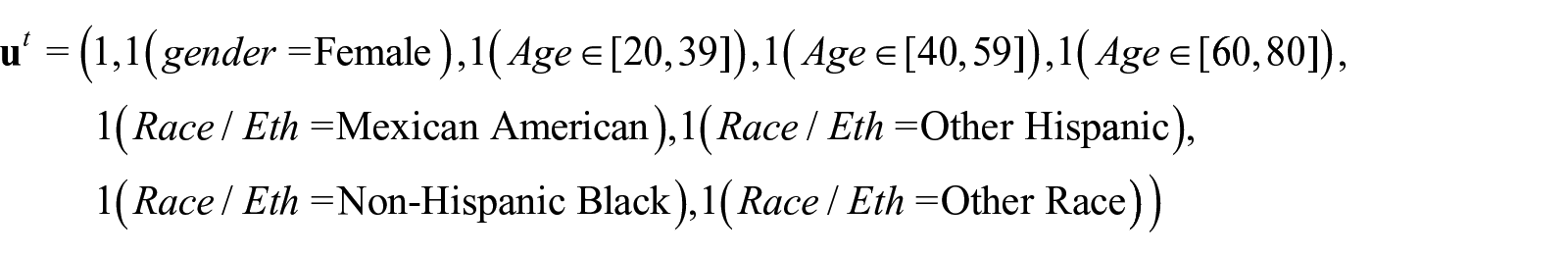
We fit the models used in the simulation study (that does not include PSUs): FULL, PSEUDO, POP, and also an extension of our method to adjust for PSU (labeled FULL.PSU) as described in Subsection 3.2. We recall that two-year NHANES cycle data contains thirty PSUs. The vector of covariates in Equation (5) in this application is,

$$\begin{array}{l}\begin{array}{l}{\mathbf{u}}^t=(1,1\left(gender=\mathrm{Female}\right),1\left(Age\in [20,39]\right),1\left(Age\in [40,59]\right),1\left(Age\in [60,80]\right),\\ 1\left(Race/Eth=\mathrm{Mexican}\mathrm{American}\right),1\left(Race/Eth=\mathrm{Other}\mathrm{Hispanic}\right),\\ 1\left(Race/Eth=\mathrm{Non-Hispanic}\mathrm{Black}\right),1\left(Race/Eth=\mathrm{Other}\mathrm{Race}\right))\end{array}\hfill \end{array}$$

Here $1(A)$ denotes the indicator function of the individual in the set $A$ . For FULL and FULL.PSU, the covariate vector to model πi $|y_i$ , in Equation (9) and (15) respectively, ${\mathbf{v}}_i$ , is set equal to ${\mathbf{v}}_i={\mathbf{u}}_i$ .

FULL and FULL.PSU results indicate that the design is informative for protein consumption. As Table 2 shows, for FULL, the posterior mean (central 95% credible intervals) of ${\kappa }_y$ , in Equation (9), is −0.17 (−0.22, −0.13); while for FULL.PSU the mean of ${\kappa }_y$ , in Equation (15), is −0.31 (−0.36, −0.26). In both cases, the CI for ${\kappa }_y$ does not contain zero.

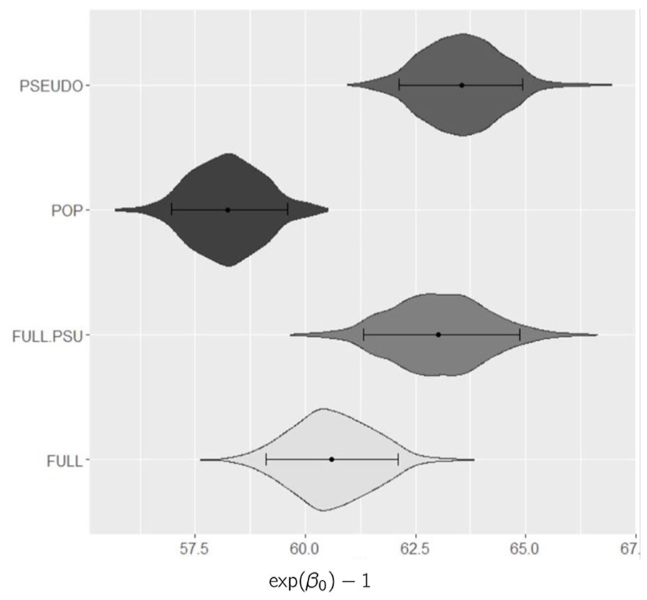
Figure 1 shows that the methods yield different inference. The figure presents violin plots representing the posterior distribution of the grams of protein consumed by participants in the reference group, that is, of $\exp \left({\beta }_0\right)-1$ , under all competing models. POP, the model ignoring the sampling weights, underestimates. The estimate under PSEUDO is the highest and its CI does not overlap FULL CI. The difference in point estimates between FULL and PSEUDO probably derives from the use of raw, noisy weights in PSEUDO. These noisy weights contain a sufficiently high variance unrelated to the response variable that at the released sample size there is estimation bias. The CIs under FULL and FULL.PSU overlap but FULL.PSU tends to yield higher standard deviations because FULL.PSU accounts for the possible non-independence of the outcomes of individuals within the same PSU. Since NHANES uses a multi-stage sampling design inference under FULL.PSU is more appropriate.

Figure 1.

Violin plots along with, mean (dot) and central 95% credible interval (horizontal line) for the expected grams of protein consumed, $exp({\beta }_0)-1$ , under all considered methods in the reference group (White male under 20).

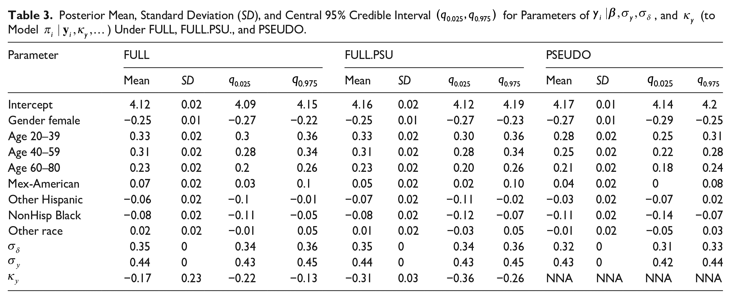
Table 3 displays mean, standard deviation, and central 95% CI for the model parameters for $y|\beta ,{\sigma }_y,{\sigma }_{\delta }$ , ${\kappa }_y$ under FULL, FULL.PSU and PSEUDO. FULL and FULL.PSU produce similar point estimates except for the intercept for which FULL. PSU yields higher standard error, or equivalently, wider credible interval. This is expected because FULL. PSU takes into account the correlation of the responses within the same PSU (95% CI for ${\sigma }_{\eta }$ in Equation (14) is $(0.02,0.05)$ ). Inference under PSEUDO is different.

Table 3.

Posterior Mean, Standard Deviation (SD), and Central 95% Credible Interval $(q_{0.025},q_{0.975})$ for Parameters of $y_i|\beta ,{\sigma }_y,{\sigma }_{\delta }$ , and ${\kappa }_y$ (to Model ${\pi }_i|{\mathbf{y}}_i,{\kappa }_y,\dots$ ) Under FULL, FULL.PSU., and PSEUDO.

Parameter	FULL				FULL.PSU				PSEUDO
	Mean	SD	$q_{0.025}$	$q_{0.975}$	Mean	SD	$q_{0.025}$	$q_{0.975}$	Mean	SD	$q_{0.025}$	$q_{0.975}$
Intercept	4.12	0.02	4.09	4.15	4.16	0.02	4.12	4.19	4.17	0.01	4.14	4.2
Gender female	−0.25	0.01	−0.27	−0.22	−0.25	0.01	−0.27	−0.23	−0.27	0.01	−0.29	−0.25
Age 20–39	0.33	0.02	0.3	0.36	0.33	0.02	0.30	0.36	0.28	0.02	0.25	0.31
Age 40–59	0.31	0.02	0.28	0.34	0.31	0.02	0.28	0.34	0.25	0.02	0.22	0.28
Age 60–80	0.23	0.02	0.2	0.26	0.23	0.02	0.20	0.26	0.21	0.02	0.18	0.24
Mex-American	0.07	0.02	0.03	0.1	0.05	0.02	0.02	0.10	0.04	0.02	0	0.08
Other Hispanic	−0.06	0.02	−0.1	−0.01	−0.07	0.02	−0.11	−0.02	−0.03	0.02	−0.07	0.02
NonHisp Black	−0.08	0.02	−0.11	−0.05	−0.08	0.02	−0.12	−0.07	−0.11	0.02	−0.14	−0.07
Other race	0.02	0.02	−0.01	0.05	0.01	0.02	−0.03	0.05	−0.01	0.02	−0.05	0.03
${\sigma }_{\delta }$	0.35	0	0.34	0.36	0.35	0	0.34	0.36	0.32	0	0.31	0.33
${\sigma }_y$	0.44	0	0.43	0.45	0.44	0	0.43	0.45	0.43	0	0.42	0.44
${\kappa }_y$	−0.17	0.23	−0.22	−0.13	−0.31	0.03	−0.36	−0.26	NNA	NNA	NNA	NNA

7. Final Discussion

LS2019 proposed a method to include the sampling weights into the likelihood to perform Bayesian inference. They mainly focus on the linear regression with fixed effects. We extended their work to account for repeated measures by including a participant-specific random effect and modeling the inclusion probability for individual $i$ , that is, πi $|{\mathbf{y}}_i$ , as a function the average of all repeated responses for individual $i$ , that is, ${\overline{y}}_i$ , but we could have used any other linear combination of the entries of ${\mathbf{y}}_i$ . Our simulation showed that (A) our proposed method, FULL, yields credible intervals with correct coverage at the cost of wider CI than if we were analyzing a SRS; (B) that this is not always the case for PSEUDO; and (C) that our method is robust against the violation of the lognormal distribution of πi $|{\mathbf{y}}_i$ that it assumes. To check (C) the simulation true inclusion probabilities, in Section 5, were generated from gamma and exponential distributions. In LS2019 the robustness against this violation was explored more deeply. For example, in Subsubsection 4.1.2 they generated the inclusion probabilities, πis, from a Beta (symmetric) distribution and, in Subsection 4.2, they used the 2013 to 2014 NHANES sampling weights as the simulation truth. Also León-Novelo and Savitsky (2023), in their Subsection 4.2, generated (correlated within cluster) sampling weights from a Dirichlet distribution. In all these simulation scenarios the Fully Bayesian method was robust against the violation of the assumed lognormal distribution of πi $|{\mathbf{y}}_i$ . We also incorporated the PSU information following León-Novelo and Savitsky (2023) in Subsection 3.2.

Our method is computationally more expensive than other approaches. We rely on Stan to cope with this limitation. The coding of our method on Stan is simple as shown in the Appendix A.4. The lognormal distribution of πi $|{\mathbf{y}}_i$ with mean a linear combination of the entries of ${\mathbf{y}}_i$ and other covariates, as shown in Equation (9), remains a computational restriction of our proposed approach. We aim to address this in future work. Another line for future work is to extend the method to binary and count responses.

In this Article, we treat the observed inclusion probabilities as known for the survey participants only. Here the inclusion probability, πi, is the joint probability of the individual being selected and responding to the survey usually computed assuming independence, as the product of each marginal probability (of inclusion and of responding). The inclusion probabilities, or equivalently the sampling weights, provided to the analyst (e.g., the NHANES dietary publicly available data) are usually adjusted for nonresponse. If the probabilities of being selected were known by the analyst while the one of being a respondent were estimated by the analyst, the estimation error of the latter could be accounted for by modeling the nonresponse probabilities.

A limitation of our simulation study in Section 5 is that it does not incorporate non-response explicitly on the data generating process. πi is defined as the probability of both being selected and responding. We could have generated both the probability of selected to be invited to participate for individual $i$ π sel,i and their probability of responding (once invited) as πR,i. Assuming independence conditioned on the response and relevant covariates, the probability of being selected or invited to participate in the survey and respond is ${\pi }_i={\pi }_{sel,i}\times {\pi }_{R,i}$ , and we would propose to pass only πi to the data analyst. In our simulation study, we directly generate πi and pass it to the analyst. Yet, if πR,i is estimated from the observed data (e.g., the probability of response for an invited person of Hispanic ethnicity is estimated as the response rate of Hispanics invited to participate), the nonresponse adjustment induces a dependence between the Hispanic participants; nonresponse estimation from common data was not explored in the simulation section. The effect of adjustment for non-response when non-response is estimated from common data is a future line of research.

A referee made the observation that if the weights are adjusting for three factors: (1) unequal probability of being invited to participate in the survey, (2) nonresponse, and (3) post-stratification, a more appropriate terminology for these weighs is “survey weights,” while “sampling weights” should be used to refer to weights adjusting for (1) only. We agree, this terminology is more descriptive of what these weights adjust for. We decided to keep the term “sampling weights” to match NHANES terminology where the sampling weights are adjusted for (1), (2), and (3).

In summary, we propose a Bayesian method to the analysis of repeated measures under informative sampling that yields appropriate point estimates (low bias and MSE) and uncertainty quantification (CI reaching nominal coverage).

References

1.
CarpenterB.GelmanA.HoffmanM.LeeD.GoodrichB.BetancourtM.BrubakerM. A.GuoJ.LiP.RiddellA.2016. “Stan: A Probabilistic Programming Language.”Journal of Statistical Software20: 1–37. DOI: https://doi.org/10.18637/jss.v076.i01.
Centers for Disease Control (CDC). 2016a. “National Health and Nutrition Examination Survey.” Available at: https://www.cdc.gov/nchs/nhanes/index.htm (accessed June 2016).
4.
Centers for Disease Control (CDC). 2016b. “CDC/NCHS/National Health and Nutrition Examination Survey Tutorials. Module 4: Variance Estimation.” Available at: https://wwwn.cdc.gov/nchs/nhanes/tutorials/Module4.aspx (accessed January 14, 2021).
5.
ChenT.-C.ClarkJ.RiddlesM. K.MohadjerL. K.FakhouriT. H.2020. “National Health and Nutrition Examination Survey, 2015–2018: Sample Design and Estimation Procedures.” DOI: https://pubmed.ncbi.nlm.nih.gov/33663649/.
6.
KimJ. K.ParkS.LeeY.2017. “Statistical Inference Using Generalized Linear Mixed Models Under Informative Cluster Sampling.”Canadian Journal of Statistics45 (4): 479–97. DOI: https://doi.org/10.1002/cjs.11339.
7.
León-NoveloL. G.SavitskyT. D.2019. “Fully Bayesian Estimation Under Informative Sampling.”Electronic Journal of Statistics13 (1): 1608–45. DOI: https://doi.org/10.1214/19-EJS1538.
8.
León-NoveloL. G.SavitskyT. D.2023. “Fully Bayesian Estimation Under Dependent and Informative Cluster Sampling.”Journal of Survey Statistics and Methodology11 (2): 484–510. DOI: https://doi.org/10.1093/jssam/smab037.
PfeffermannD.KriegerA. M.RinottY.1998. “Parametric Distributions of Complex Survey Data Under Informative Probability Sampling.”Statistica Sinica8: 1087–114. DOI: http://www.jstor.org/stable/24306526.
11.
Rabe-HeskethS.SkrondalA.2006. “Multilevel Modelling of Complex Survey Data.”Journal of the Royal Statistical Society Series A: Statistics in Society169 (4): 805–27. DOI: https://doi.org/10.1111/j.1467-985X.2006.00426.x.
ToozeJ. A.GrunwaldG. K.JonesR. H.2002. “Analysis of Repeated Measures Data with Clumping at Zero.”Statistical Methods in Medical Research11 (4): 341–55. DOI: https://doi.org/10.1191/0962280202sm291ra.
14.
ToozeJ. A.KipnisV.BuckmanD. W.CarrollR. J.FreedmanL. S.GuentherP. M.Krebs-SmithS. M.SubarA. F.DoddK. W.2010. “A Mixed-Effects Model Approach for Estimating the Distribution of Usual Intake of Nutrients: The NCI Method.”Statistics in Medicine29 (27): 2857–68. DOI: https://doi.org/10.1002/sim.4063.
15.
ToozeJ. A.MidthuneD.DoddK. W.FreedmanL. S.Krebs-SmithS. M.SubarA. F.GuentherP. M.CarrollR. J.KipnisV.2006. “A New Statistical Method for Estimating the Usual Intake of Episodically Consumed Foods with Application to Their Distribution.”Journal of the American Dietetic Association106 (10): 1575–87. DOI: https://doi.org/10.1016/j.jada.2006.07.003.
16.
ZangenehS. Z.LittleR. J. A.2015. “Bayesian Inference for the Finite Population Total from a Heteroscedastic Probability Proportional to Size Sample.”Journal of Survey Statistics and Methodology3 (2): 162–92. DOI: https://doi.org/10.1093/jssam/smv002.