
Abstract
Sensor placement (SP) and informative path planning (IPP) problems are prevalent in environmental monitoring. These problems require gathering the most informative data from a limited number of sensing locations, but existing solutions face a difficult trade-off. Existing methods are often either computationally efficient but less informative, or more informative but too computationally expensive for practical use, especially on resource-constrained robots. Furthermore, many approaches are limited by requiring discretization of the environment or relying on slow, derivative-free optimization techniques. This paper introduces a novel, computationally efficient variational formulation for the SP problem. Our approach is differentiable with respect to the sensing locations, enabling fast gradient-based optimization in continuous spaces and delivering performance comparable to MI-based methods at a fraction of the computational cost. We establish our formulation as a special case of sparse Gaussian processes (SGPs). This connection allows us to generalize the method to solve the IPP problem for single and multi-robot systems, efficiently incorporating differentiable path constraints and diverse sensor types. The approach is validated through extensive benchmarks and field experiments with an autonomous surface vehicle (ASV) and an autonomous underwater vehicle (AUV). We also provide SGP-Tools—an open-source Python library—and a companion ROS 2 package for Ardupilot-based mobile robots.
Introduction
Motivation: Understanding and predicting environmental phenomena—such as temperature, ozone concentration, soil chemistry, ocean salinity, and fugitive gas density—are central to meteorology and climate change research (Jakkala and Akella, 2022; Krause et al., 2008; Ma et al., 2017; Suryan and Tokekar, 2020; Whitman et al., 2021). Deploying dense, static sensor networks to monitor these phenomena across an entire environment is often prohibitively expensive, and in many cases physically infeasible. The sensor placement (SP) problem addresses this limitation by selecting a small number of strategic sensor locations that enable accurate estimation of the phenomenon everywhere.
In dynamic or hard-to-access environments, mobile robots (Figure 1) can act as sensors, collecting data while moving through the environment. This leads to the informative path planning (IPP) problem, a generalization of SP that incorporates constraints—such as travel distance, time budgets, and spatial boundaries—when determining where and how to collect data. An autonomous surface vehicle mapping a lake during our field trials.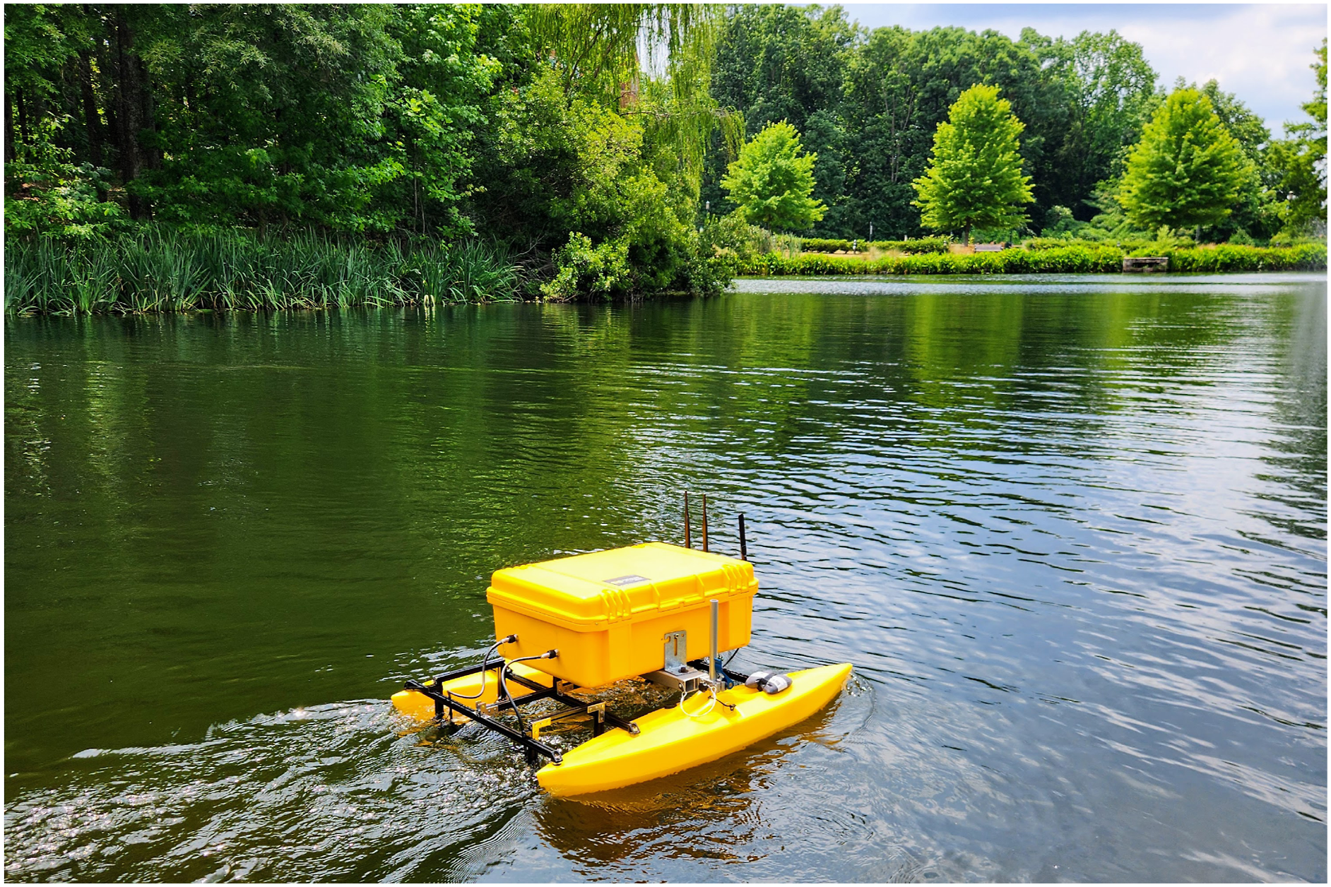
Applications: SP and IPP are fundamental to a wide range of domains: inspection and monitoring tasks (Zhu et al., 2021), learning dynamical systems from sparse data (Buisson-Fenet et al., 2020), persistent ocean monitoring using underwater gliders (Smith et al., 2011), gas-source localization in oil fields (Jakkala and Akella, 2022), and active learning for aerial semantic mapping (Rückin et al., 2022). These applications share a common challenge: producing high-quality sensing strategies with minimal prior knowledge about the phenomenon and with tight computational budgets.
Existing approaches: Many SP and IPP methods choose sensing locations by maximizing variance or mutual information (MI). Variance is computationally efficient but may yield less informative locations (Krause et al., 2008), whereas MI is more informative but computationally expensive, making it impractical for resource-limited robots.
Optimization methods for these objectives include integer programs and greedy algorithms (Krause and Guestrin, 2011; Ma et al., 2018), which require discretizing the environment—restricting solutions to predefined points and potentially degrading sensing quality. Derivative-free optimizers (e.g., genetic algorithms, Bayesian optimization (Francis et al., 2019; Hitz et al., 2017; Popović et al., 2020; Vivaldini et al., 2019)) can operate in continuous spaces but are slow, especially when paired with MI. Gradient-based approaches (Asgharivaskasi et al., 2022; McCammon and Hollinger, 2021; Ott et al., 2024a) have also been investigated for IPP, though some target different problem settings or emphasize variance-based objectives to improve computational efficiency.
Our approach: We propose a novel variational formulation of the SP problem that yields an optimal sparse distribution of sensing locations. This formulation matches or exceeds the performance of MI-based methods while being significantly faster, due to its differentiability with respect to sensor locations. Differentiability enables the use of efficient gradient-based optimizers (e.g., gradient descent, conjugate gradient descent) in continuous domains—dramatically reducing computation time compared to derivative-free methods.
A key insight is that our formulation is a special case of sparse Gaussian processes (SGPs) (Titsias, 2009), allowing us to directly draw on established SGP results. Leveraging this connection, we generalize our SP framework to IPP, incorporating differentiable path constraints for efficient planning in complex spatio-temporal and 3D environments.
Contributions
Our core contributions to the fields of sensor placement (SP) and informative path planning (IPP) are as follows: 1. We introduce a novel variational formulation for the SP problem, from which we derive an optimal sparse distribution that yields the solution sensing locations. 2. We establish a crucial connection, demonstrating that our variational SP formulation is a special case of sparse Gaussian processes (SGPs). This insight allows us to leverage key results from the SGP literature to enhance our SP approach. 3. We present SP algorithms that leverage our variational formulation with efficient gradient-based optimization techniques, enabling fast SP in both continuous and discrete spaces. 4. We generalize our SP approach to model both point and non-point field-of-view (FoV) sensors, thereby enabling us to accommodate point sensors such as temperature probes and non-point sensors such as thermal vision cameras. 5. We further generalize our SP approach to address single and multi-robot IPP, capable of modeling both discrete and continuous sensing robots while incorporating differentiable path constraints like distance budgets and boundary limits. 6. We validate the performance and advantages of our approaches through multiple benchmarks and demonstrations, including field experiments with an autonomous surface vehicle (ASV) and an autonomous underwater vehicle (AUV). 7. We provide an open-source Python library—SGP-Tools
1
and a companion ROS 2 package
2
, designed for deployment on ArduPilot-based robotic platforms.
The paper is structured as follows. We begin in Problem statements section by formally posing the sensor placement (SP) and informative path planning (IPP) problems. The Preliminaries section provides essential background on Gaussian processes and mutual information.
The Method: Differentiable sensor placement section introduces our novel SP formulation and discusses its various generalizations. (Note: The foundational aspects of this formulation, corresponding to Contributions 1, 2, and 3, have previously appeared as an arXiv preprint (Jakkala and Akella, 2023)).
We then extend our SP formulation to address IPP in the Method: Differentiable informative path planning section. (These IPP extensions, along with sensor generalizations and initial experiments—Contributions 4, 5, and part of 6—were previously published as a conference paper (Jakkala and Akella, 2024)).
The Experiments section presents comprehensive benchmarks and experimental results validating our proposed approaches for both SP and IPP. The Related Work section provides an overview of related work. Finally, the Conclusion section offers conclusions and outlines directions for future work.
A further generalization of our approach addressing adaptive IPP has been recently published (Jakkala and Akella, 2025) and extends the scope of this article; see Figure 2. Roadmap of our research, showing its key components. The core contributions (blue and green) are covered in this article, with the purple component illustrating an extension derived from this foundational research.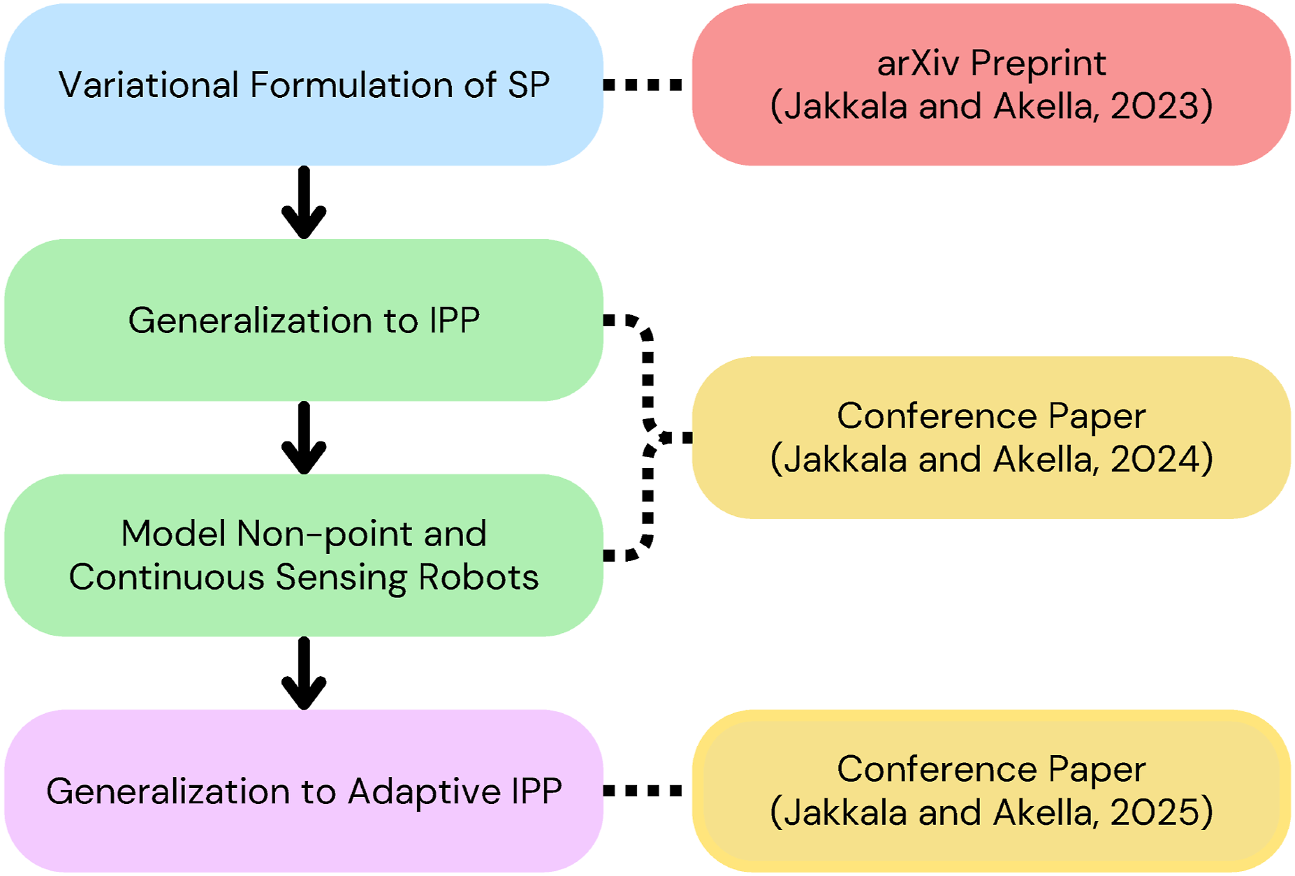
Problem statements
Environmental monitoring often involves estimating spatially, or spatiotemporally, correlated phenomena (e.g., temperature, chlorophyll concentration) over a domain
In this work, we consider the setting where only a sparse set of labeled data or prior domain knowledge about environmental correlations is available, typically derived from an initial pilot survey or pre-existing datasets (Kemna et al., 2018).
Sensor placement problem: The SP problem seeks a sparse set of s stationary sensor locations
We model the phenomenon using a Gaussian process (GP, Rasmussen and Williams, 2005). Since direct minimization of reconstruction error (e.g., root-mean-square error (RMSE)) is infeasible without dense ground truth labels, we instead maximize a computable information-theoretic criterion
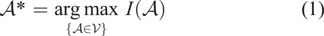
We consider both continuous space SP, where sensors can be placed anywhere in
Informative path planning problem: IPP extends SP from selecting stationary sensing locations to planning a set of paths
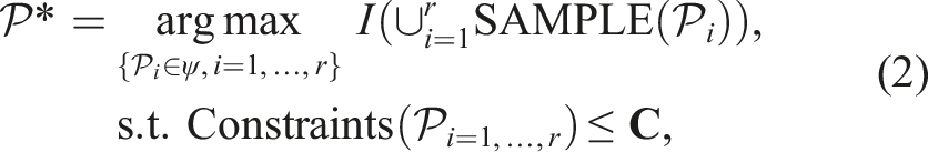
We distinguish between discrete-sensing platforms, which gather measurements only at waypoints along the path (e.g., soil core sampling for nutrient analysis), and continuous-sensing platforms, which acquire data continuously along the path, for example, Binney et al. (2010). The definition of SAMPLE(⋅) is adapted to the sensing modality.
Preliminaries
This section provides essential background on Gaussian processes (GPs) and mutual information (MI), which are foundational to understanding our proposed approach for sensor placement (SP) and informative path planning (IPP).
Gaussian processes
Gaussian processes (GPs, Rasmussen and Williams, 2005) are a non-parametric Bayesian method widely used for regression, classification, and generative tasks. For a regression task, given a training set
GPs model such datasets by imposing a GP prior over the space of functions, specifically assuming a prior distribution over the function of interest
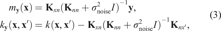
The parameters of the kernel function are optimized using Type II maximum likelihood (Bishop, 2006) to enable the GP to accurately predict the training data labels. The GP’s posterior mean and covariance functions, used for predictions, are computed as:
Mutual information
Mutual information (MI) has been a cornerstone in early SP approaches, as demonstrated by Caselton and Zidek (1984). They framed the SP problem as maximizing the MI between the unobserved locations in the environment
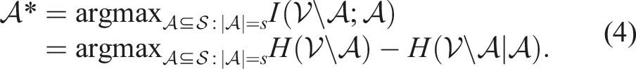
In this formulation,
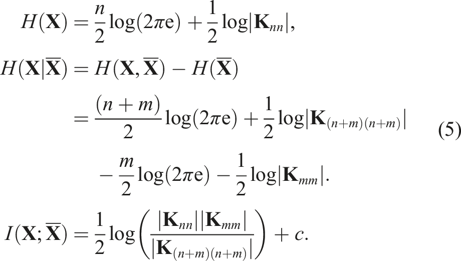
Here,
A significant challenge with MI-based formulations is their inherent definition on discrete sets of locations, necessitating the discretization of the environment into n locations. Moreover, the determinant term |
Given that MI formulations for SP are typically set functions (Caselton and Zidek, 1984; Krause et al., 2008), most existing approaches rely on greedy algorithms or derivative-free black-box optimizers like genetic algorithms (Hitz et al., 2017) or Bayesian optimization (Francis et al., 2019) to find optimal sensing locations. However, these methods demand numerous, computationally intensive MI evaluations, which severely restricts the scalability of SP and IPP approaches that utilize MI.
Despite these limitations, MI can also be applied to Gaussian processes, which are capable of modeling environments in a continuous space, effectively representing an infinitely fine discretization (Baker, 1970). While many approaches utilize GPs to compute covariances for MI, they often solve the problem in a discrete space. However, the MI formulation for GPs is fully differentiable with respect to sensing locations in continuous spaces, making it amenable to faster gradient-based optimization methods. Nevertheless, the computational expense associated with determinant terms in the MI calculation persists. To address these fundamental limitations of existing MI-based methods, this article introduces a novel variational approximation-based formulation for the SP problem that enables computationally efficient optimization using gradient-based approaches.
Method: Differentiable sensor placement
This section details our novel, computationally efficient variational formulation for the sensor placement (SP) problem, which is differentiable with respect to sensing locations. Then we introduce three algorithms—Continuous-SGP, Greedy-SGP, and Discrete-SGP—to address both continuous and discrete space SP problems. We also present a method for modeling non-point field of view (FoV) sensors.
Theoretical foundation
We first address the SP problem, which requires us to identify strategic sensing locations within an environment. The goal is to ensure that data collected from these locations enables accurate reconstruction of the monitored data field.
We model the underlying data field as a stochastic process using a Gaussian process (GP). Note that, despite their name, GPs are not limited to modeling Gaussian distributed functions. We define a GP
To determine the optimal sensor placements, we approximate the GP
We formulate the sparse distribution
It is important to recognize that the specific values of the inducing latent variables
To optimize this sparse distribution

The formulation of
A GP is fundamentally comprised of two essential components: • The kernel function: This function defines a prior in the function space, essentially dictating the smoothness and correlation properties of the solution function. While it establishes how labels are correlated, it does not determine the actual values of the labels at each location. • The training set: This set provides concrete observations, allowing us to constrain the GP solution. Combined with the kernel function, the training set enables the GP to focus on a smaller subset of functions that not only satisfy the observed labels but also adhere to the smoothness properties defined by the kernel.
However, our SP problem does not assume access to a dense training set. Consequently, we cannot directly incorporate
The inclusion of zero-labeled data in our training set has two significant implications for our approach: • A definition of a full GP: The zero-labeled data ensures that the target GP • A distribution over inducing locations: The inclusion of zero-labeled data enables us to optimize the sparse approximation
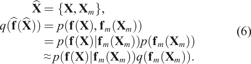
To define both the full GP
We now turn our attention to optimizing the sparse approximation

Note that the above uses the reverse KL-divergence, making it computationally feasible to optimize (Bishop, 2006). By substituting the expressions for the full GP and the sparse approximation into the above ELBO, we obtain the following
3
:
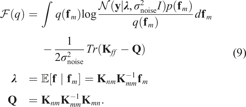
Here, σnoise is the data noise, and the subscripts of the covariance matrix

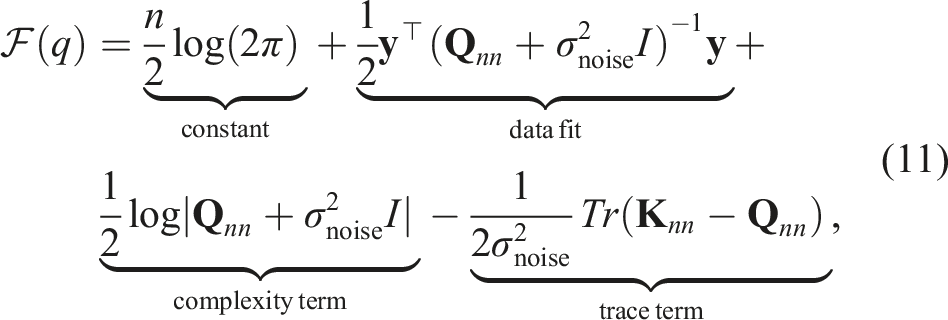
The ELBO • Data Fit Term: This term quantifies how well the model fits the observed training data. In our specific formulation, since the labels in our uninformative training set are all set to zero, this data fit term becomes zero and contributes no information regarding the phenomenon’s actual values. • Complexity Term: This term encourages the inducing points (i.e., the input locations • Trace Term: This term represents the sum of the variances of the conditional distribution p(
The optimized inducing points
Furthermore, a significant advantage of this formulation is that the inducing points can be optimized in continuous spaces. This allows for the use of efficient gradient-based optimization approaches, such as gradient descent or Newton’s method. This continuous optimization capability makes our approach significantly faster compared to discrete SP methods and readily scales to complex 3D and spatiotemporal environments.
The presented result can be interpreted as a special case of sparse Gaussian processes (SGPs) (Snelson and Ghahramani, 2006; Titsias, 2009), where the training set inputs correspond to the locations within the monitored data field, and all labels are set to zero. Specifically, our formulation closely aligns with that of the sparse variational Gaussian process (SVGP). As such, we also refer to our approach as SGP-based SP. Further details regarding this derivation are provided in Appendix A.
To summarize our approach to the SP problem: we started by modeling the data field of interest as a stochastic process using a GP. Subsequently, we developed an approximate inference-based formulation and derived the SP solution through variational inference. We then established a connection to the existing SGP literature, highlighting that SGPs inherently solve the sensor placement problem in a supervised learning context. Our formulation further demonstrates that when the kernel hyperparameters are known, SGPs can be trained in an unsupervised manner by setting the training set labels to zero and optimizing the SP locations.
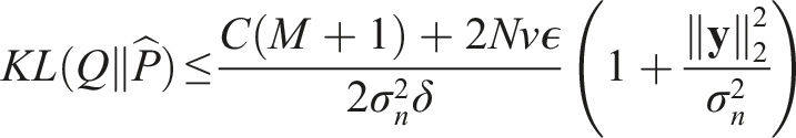
This formulation offers the significant advantage of leveraging the extensive SGP literature to tackle various complexities and variants of the SP problem. For example: • For environments requiring a large number of sensor placements, we can integrate our approach with stochastic gradient optimizable SGPs (Hensman et al., 2013; Wilkinson et al., 2021). • To efficiently optimize sensor placements in spatiotemporally correlated environments, we can employ spatiotemporal SGPs (Hamelijnck et al., 2021) in conjunction with our method. • Moreover, the detailed analysis of the SVGP lower bound by Bauer et al. (2016) offers valuable insights into how the inducing points (i.e., sensing locations) and hyperparameters influence the solution, and how they can be more effectively optimized. • Additionally, this formulation enables us to upper bound the KL divergence between the sparse approximation and the ground truth full GP modeling the underlying phenomenon in the environment. This bound can be used to assess the quality of the sparse approximation computed from the solution sensor placements:
(Burt et al., 2020) Suppose N training inputs are drawn i.i.d according to input density p( Here, k represents the k-value in the k-determinantal point process, and k represents the kernel function. In our sensor placement problem, Q is equivalent to the sparse approximation that can be used to predict the state of the whole environment from sensor data collected at the inducing points, and • The above theorem also suggests an asymptotic convergence guarantee, that is, as the number of sensing locations increases, the probability of the sparse approximation being exact approaches one. Please refer to Appendix A for additional theoretical analysis of the approach.
Continuous-SGP: Continuous space solutions
Algorithm 1—Continuous-SGP—leverages our differentiable variational formulation to solve the SP problem in continuous spaces. The process begins by sampling random unlabeled locations within the monitoring environment’s boundaries. These locations, denoted as
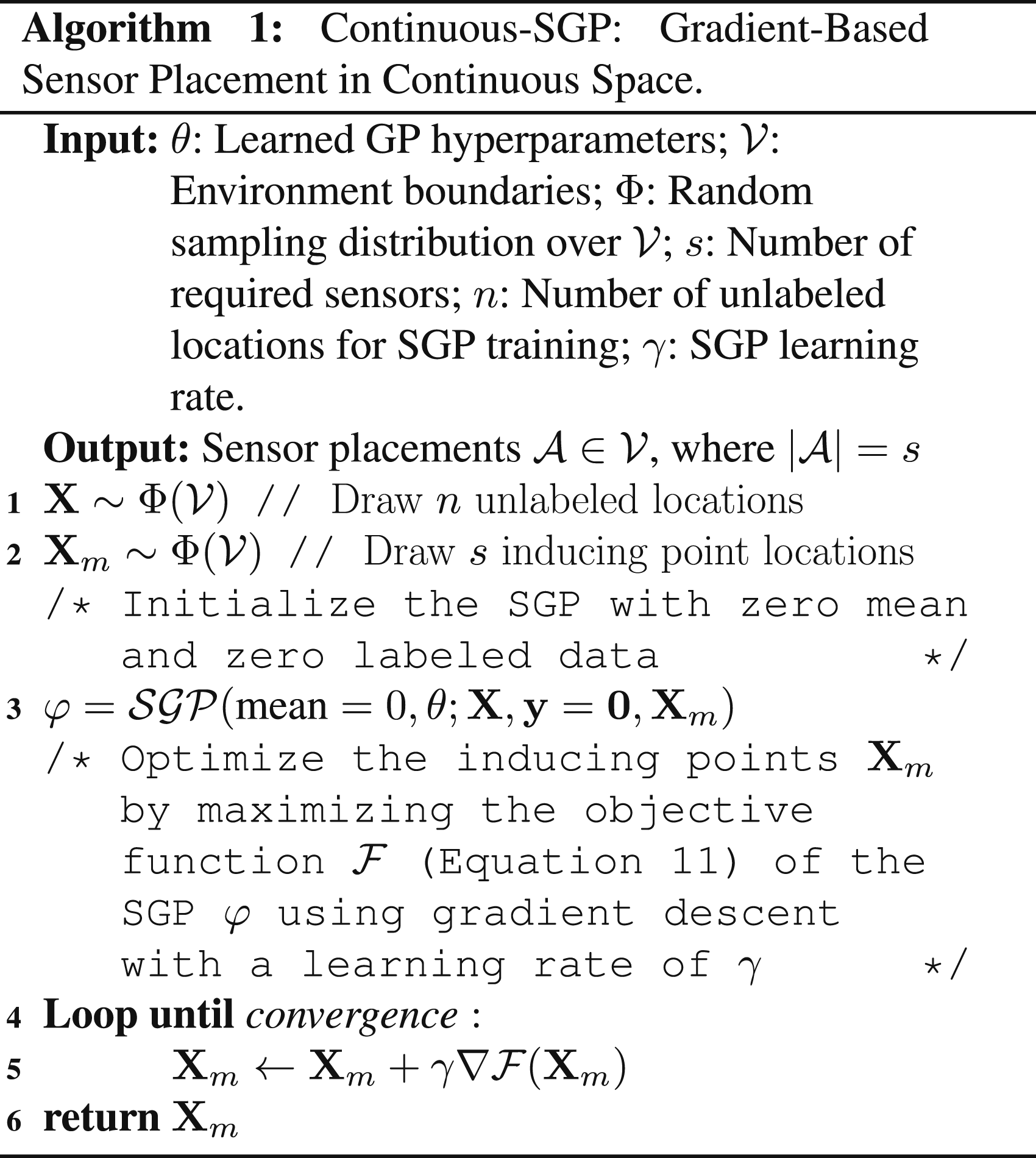
Next, we initialize the inducing points
An SGP is then initialized using the sampled unlabeled training set and the inducing points. Specifically, we utilize the sparse variational free energy-based Gaussian process (SVGP), which aligns with our variational formulation. However, any SGP approach is compatible with our algorithm for solving the SP problem.
The inducing point locations of the SGP are subsequently optimized by maximizing the complexity and trace terms of the lower bound
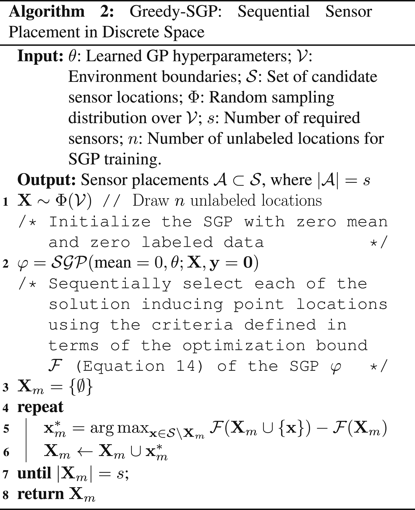
Greedy-SGP: Greedy discrete space solutions
For scenarios requiring SP solutions constrained to a discrete set of candidate locations, the Greedy-SGP approach generalizes the inducing points selection method from (Titsias, 2009) to accommodate non-differentiable data domains.
As outlined in Algorithm 2, this approach sequentially selects inducing points
In each iteration, we select the point

Comparison with mutual information: The Greedy-SGP approach shares interesting similarities with Mutual Information (MI)-based SP methods, such as that by Krause et al. (2008). Their MI approach uses a full GP to evaluate MI between sensing locations and the monitored environment, greedily selecting locations based on the following criterion:

where

Here, the first Kullback-Leibler (KL) term quantifies the divergence between the sparse distribution q over f
i
(the latent variable corresponding to
A key distinction is that Greedy-SGP utilizes computationally efficient cross-entropy terms, whereas the MI approach relies on the expensive entropy term
Discrete-SGP: Gradient-based discrete space solutions
The inherent sequential nature of greedy selection algorithms poses a limitation: a sequentially optimized solution might be improved by replacing existing locations with others from the candidate set. Optimizing all sensing locations simultaneously, by accounting for their combined effect, can yield a superior solution.
The Discrete-SGP approach (Algorithm 3) addresses this by first optimizing all inducing points in continuous space using gradient descent, then mapping this continuous solution to the discrete candidate set
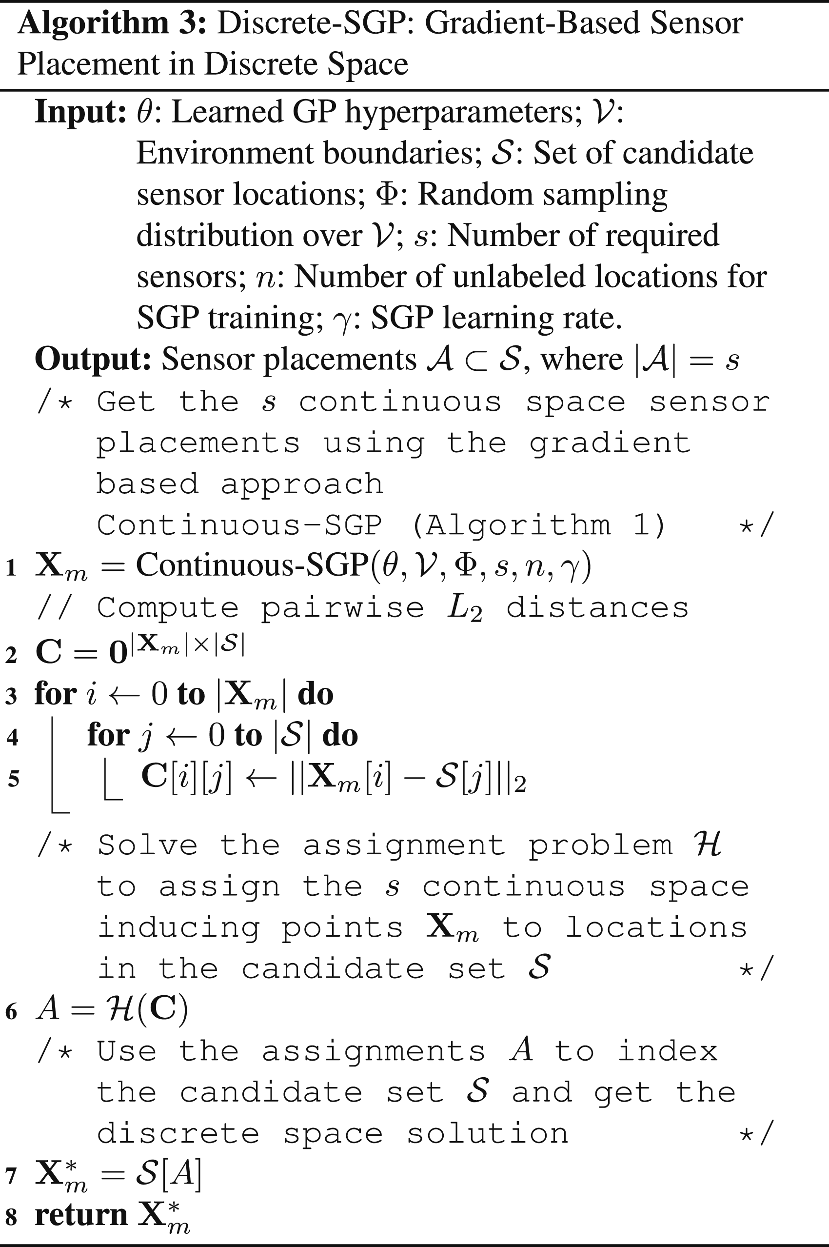
The assignment problem’s solution identifies points in the discrete candidate set that are closest to the continuously optimized solution set. This gradient-based discrete solution can be superior to greedy solutions because the points are optimized simultaneously. Although susceptible to local optima, our experiments show that gradient-based discrete solutions are comparable to or better than greedy solutions, while being substantially faster to optimize.
Non-point field of view sensors
Thus far, our discussion has focused on point sensors, which sense data at a single location (e.g., a temperature probe). However, many real-world sensors, such as thermal vision cameras, have a non-point field of view (FoV) that covers a region, often proportional to the distance from the sensor. While optimizing for point sensors and then deploying non-point FoV sensors is possible, explicitly optimizing for non-point FoV sensors can yield more informative solutions. A key advantage of our formulation is its ability to leverage the properties of GPs and SGPs to model such sensors. We detail two such properties:
Expansion transformation T
A challenge arises because the size of the covariance matrix, computed among the m × p transformed inducing points, can become computationally infeasible for inversion as p increases.
Aggregation transformation
Specifically, after applying Texp to create
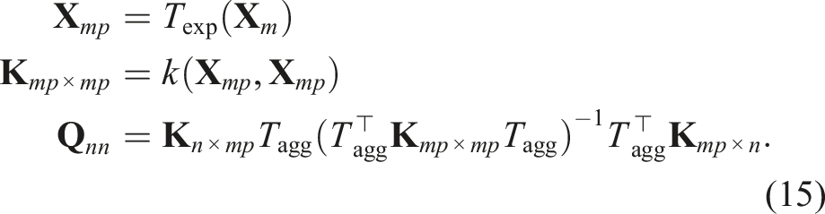
Here,
The aggregation transformation effectively reduces the matrix inversion cost from An illustration of the expansion and aggregation transformations used to model non-point FoV sensors.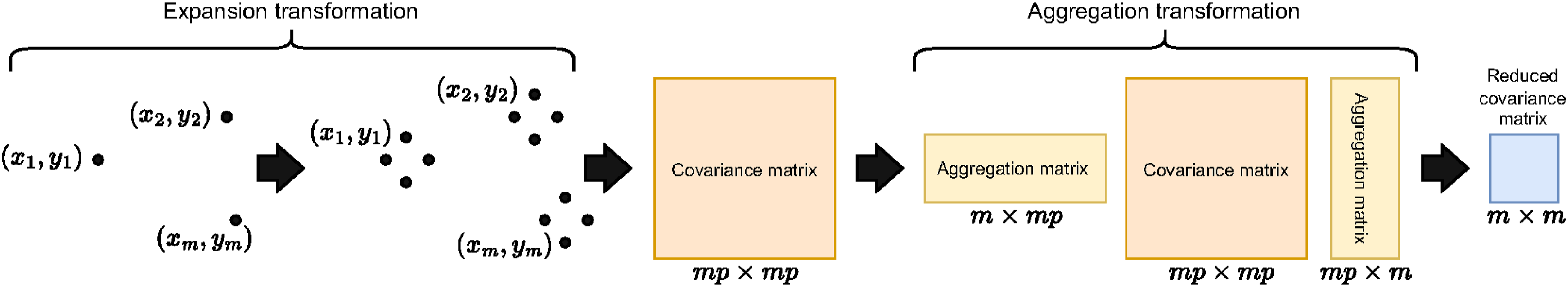
This method’s flexibility extends to modeling sensors like cameras, whose FoV scales with distance from the ground. This can be achieved by parameterizing inducing points in 3D space, using the z-axis distance to scale the area covered by the p auxiliary points approximating the FoV. Furthermore, inducing points can be parameterized with auxiliary dimensions to optimize other sensor placement aspects, such as 3D orientation or data sampling resolution. This property also enables modeling sensors with integrated observations, like gas sensors (Jakkala and Akella, 2022; Longi et al., 2020), where data is represented as
Method: Differentiable informative path planning
The informative path planning (IPP) problem extends SP by requiring the determination of informative sensing locations while simultaneously satisfying path-related constraints. Our SP formulation offers two key advantages for addressing IPP: full differentiability with respect to sensing locations and the ability to achieve informative sensing comparable to mutual information (MI)-based methods but at a significantly reduced computational cost. This section demonstrates how these features are leveraged to generalize our SP formulation to solve single and multi-robot IPP problems, including the modeling of continuous sensing robots.
Single-robot IPP
For the most basic IPP variant—finding the shortest path for a single robot to visit all sensing locations—we employ a traveling salesperson problem (TSP) solver (Perron and Furnon, 2019). We first obtain s sensor placement locations using the Continuous-SGP approach. An (approximate) TSP solver, modified to allow arbitrary start and end nodes, then generates a path
More critically, our approach excels at addressing constrained IPP variants, such as those with distance budget limits. Traditional methods often iterate through sequential selection of sensing locations and path finding, which can lead to suboptimal utilization of the available distance budget. These approaches prioritize satisfying the budget over maximizing information gain by not considering replacements for already selected locations.
We overcome this limitation by leveraging the full differentiability of the SGP’s optimization objective
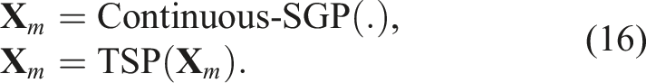
Furthermore, we can impose constraints directly on the solution paths. This is achieved by initially solving the TSP on the SGP’s initial inducing points
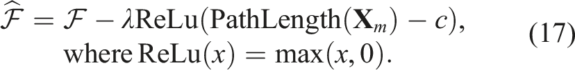
Here, PathLength (
Additional path constraints, such as limits on velocity or acceleration, can be accommodated by appropriate path parameterizations (e.g., splines parameterized by inducing points). Predefined start and end points can also be trivially enforced by freezing gradient updates for the corresponding initial and final inducing points and employing an appropriate TSP solver.
Multi-robot IPP
Our approach extends naturally to the multi-robot constrained IPP problem. This is achieved by increasing the total number of inducing points in the SGP. For r robots, each requiring s sampling locations, we initialize r × s inducing points in the environment. An initial set of r paths is then generated by solving the vehicle routing problem (VRP, Toth and Vigo, 2014), a generalization of TSP for multiple vehicles. These paths are subsequently resampled to ensure each has s points, forming an ordered set of r × s initial sensing locations.
The SGP is initialized with these r × s inducing points. Path constraints, operating on each individual path, are then added to the objective function
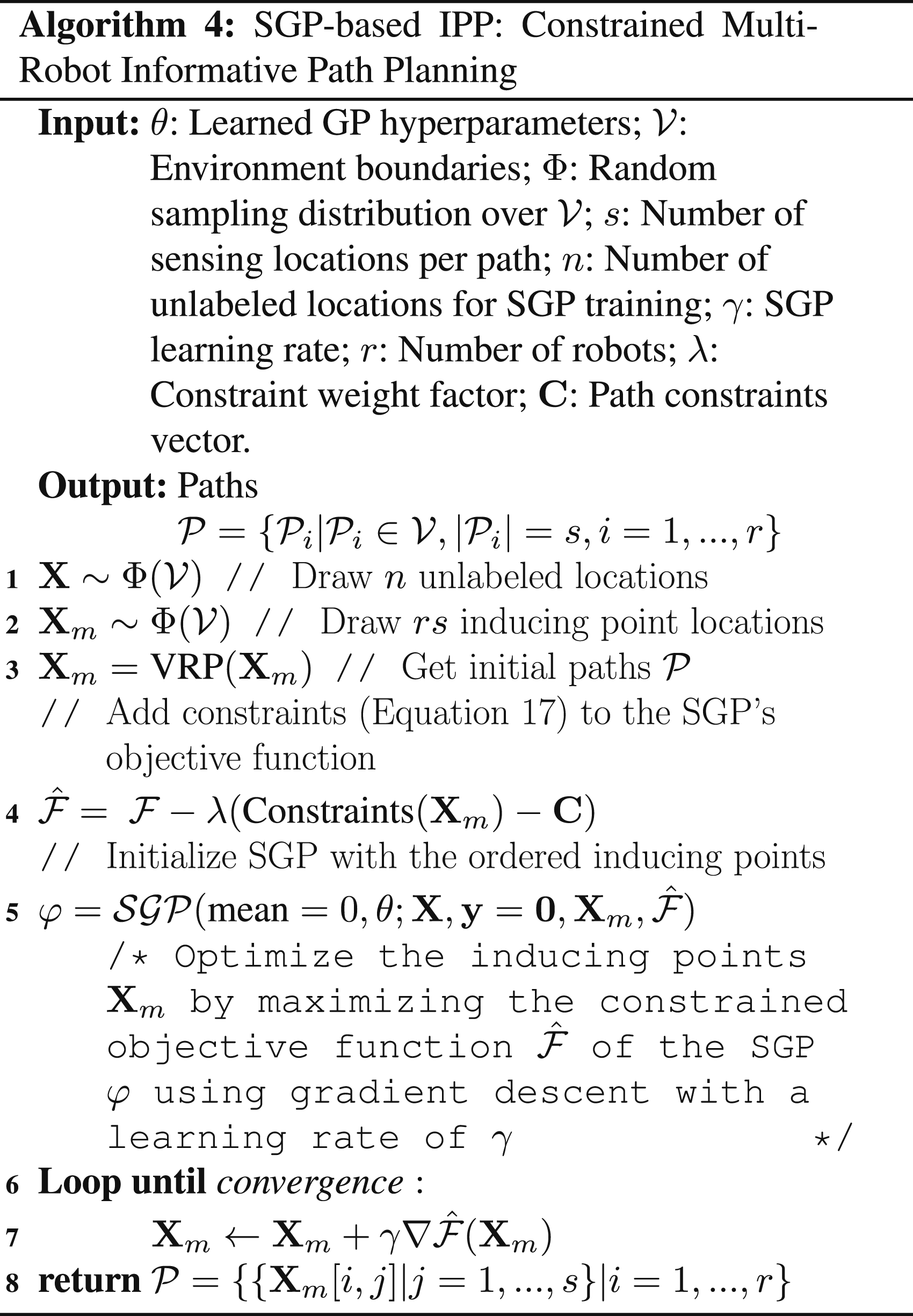
Continuous sensing robots
Many real-world sensors, such as temperature probes and gas sensors, collect data continuously along a robot’s path. This often-overlooked aspect of IPP is effectively modeled by leveraging the expansion transformation Texp and aggregation transformation Tagg, originally developed for non-point FoV sensors.
Instead of mapping each inducing point to an area representing a sensor’s FoV, we use the expansion transformation to interpolate p auxiliary inducing points between consecutive pairs of the original m inducing points along the path. This ensures that our method accounts for the information acquired continuously along the entire path, rather than just at its vertices. Subsequently, the aggregation transformation is applied to the relevant covariance matrices, which significantly reduces the computational cost of matrix inversion.
Experiments
In this section, we demonstrate the performance of the SGP-based methods for sensor placement (SP; Sensor placement) and informative path planning (IPP; Informative path planning). This includes benchmarks with multiple baseline approaches and experiments demonstrating the methods in various environments, including spatiotemporal and 3D settings, as well as field experiments.
We benchmarked the methods on four bathymetry datasets—Mississippi (NOAA, 2007), Nantucket (NOAA, 2018), Virgin Islands (NOAA, 2013), and Wrangell (NOAA, 2023)—collected by the National Oceanic and Atmospheric Administration (NOAA). The datasets are representative of real-world environments that necessitate deploying SP and IPP methods. Moreover, the datasets have densely sampled labeled data, allowing us to validate the performance of the methods thoroughly. The normalized ground truth data from each dataset is shown in Figure 42 in the Appendix.
For each dataset, we used 1000 random sampled data points to learn the kernel function parameters. The optimized kernel function was used to compute mutual information (MI) for MI-based baseline approaches, and to compute the SGP-based approaches’ objective function.
To obtain a method’s data field reconstruction estimate, the solution sensing locations from the method, along with their corresponding ground truth labels were collected. The collected data and the optimized kernel function were then used to initialize a Gaussian process (GP). This GP was then used to estimate the state of the data field at all remaining unvisited locations.
Since GPs are non-parametric, this method ensures that only the hyperparameters (i.e., the kernel parameters and data likelihood) and the data collected from the solution paths are used to compute the data field reconstruction. We used a radial basis function (RBF) kernel (Rasmussen and Williams, 2005) in all the benchmarks and trained the GPs using L-BFGS-B gradient-based optimizer (Nocedal and Wright, 2006) unless stated otherwise.
We evaluate the solution quality of each method using three standard metrics—root-mean-square error (RMSE) (Equation (18a)), standardized-mean-square error (SMSE) (Equation (18b)), and negative log predictive density (NLPD) (Equation (18c)), and the algorithm runtime:
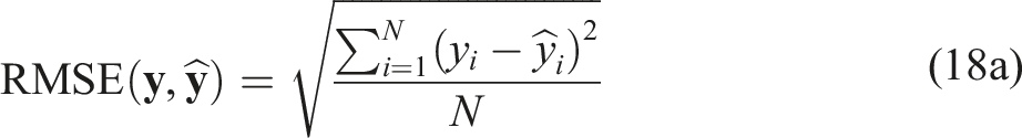
Here,
RMSE only considers the predicted labels to determine the solution quality. SMSE and NLPD incorporate the predicted variance to reduce the importance of predictions that were randomly guessed. All benchmark experiments were repeated 10 times and executed on computing nodes with 12 cores (Intel(R) Xeon(R) Gold 6154 3.00 GHz CPU) and 128 GB of RAM.
Sensor placement
We first establish the informativeness of the solutions obtained using the SGP-based SP approaches and demonstrate their runtime advantages. Next, we benchmark the performance impact of varying the number of candidate locations in a MI-based approach and the impact of various gradient-based optimizers on our approach. We then showcase the SP approach with a non-point sensing model in an environment with obstacles. Following that, we present the method in a non-stationary environment.
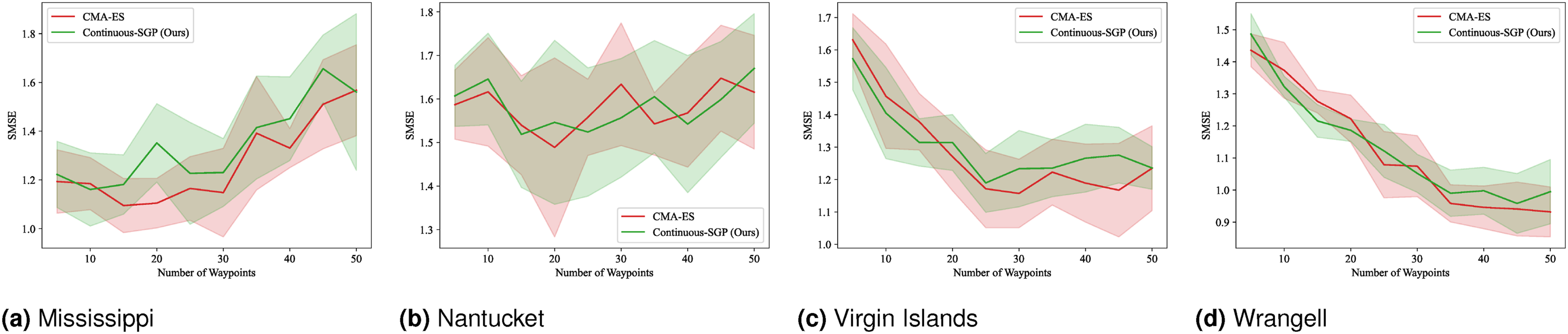
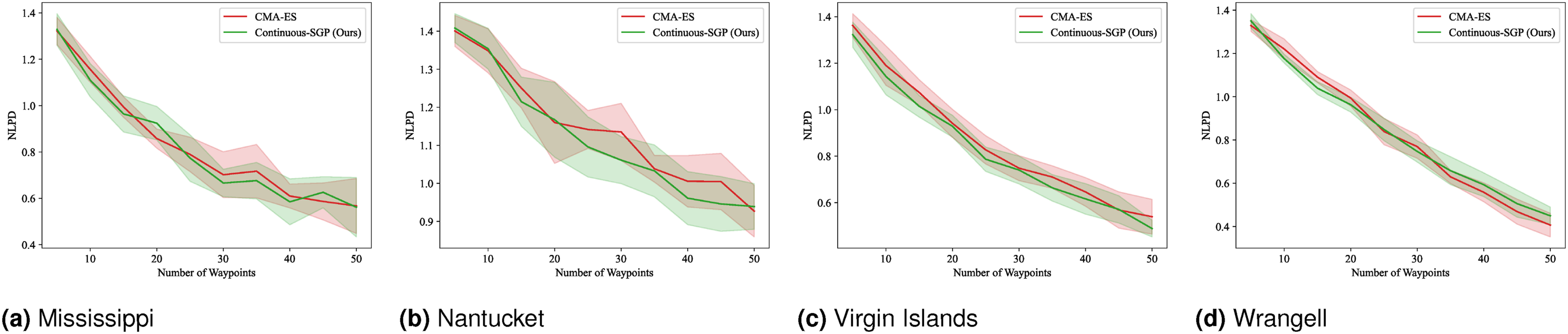
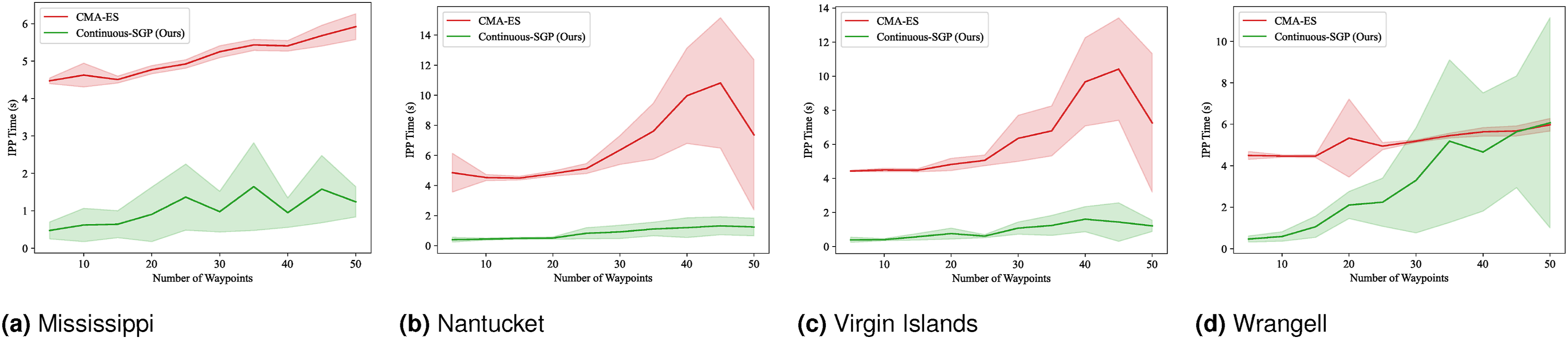
(Benchmark 1) Sensor placement: We benchmark the SP approaches, which are equivalent to the IPP approaches with a point sensing model and without any distance budget constraints. The benchmark includes discrete space methods—Discrete-SGP (Section Discrete-SGP: Gradient-based Discrete Space Solutions), Greedy-SGP (Section Greedy-SGP: Greedy Discrete Space Solutions) and Greedy-MI (Krause et al., 2008)—and continuous space methods—Continuous-SGP (Section Continuous-SGP: Continuous Space Solutions), CMA-ES (Hitz et al., 2017), BO (Francis et al., 2019; Lin et al., 2019), and Myopic (Chen et al., 2022).
Continuous-SGP uses L-BFGS-B to optimize the objective function (Equation (11)) from our variational formulation to select the sensing locations. Discrete-SGP uses the Continuous-SGP approach to find a continuous space solution and maps the solution to the candidate set to get the discrete space solution. Greedy-SGP uses a greedy algorithm to maximize the objective function (Equation (11)) from our variational formulation. Greedy-MI uses a greedy algorithm to maximize MI. CMA-ES (covariance matrix adaptation evolution strategy) employs a genetic algorithm to maximize MI. BO uses Bayesian optimization to maximize MI. Finally, the Myopic planner maximizes MI using a sampling technique (Chen et al., 2022). We chose these baselines as they are closely related approaches that address the SP problem.
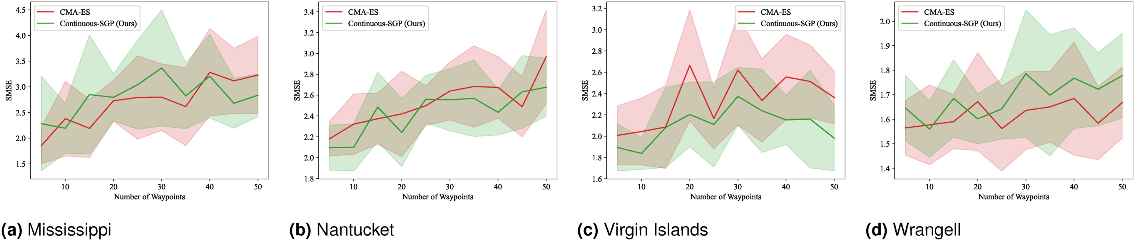
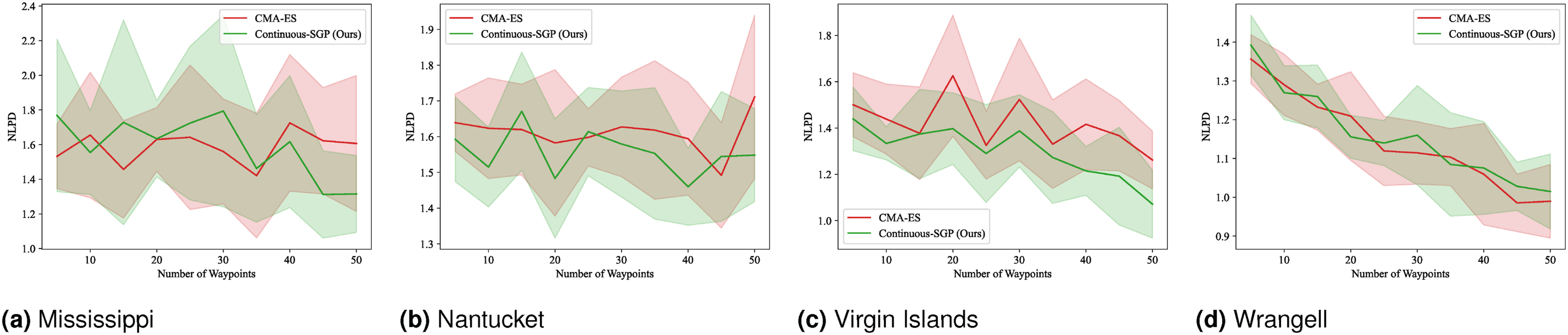
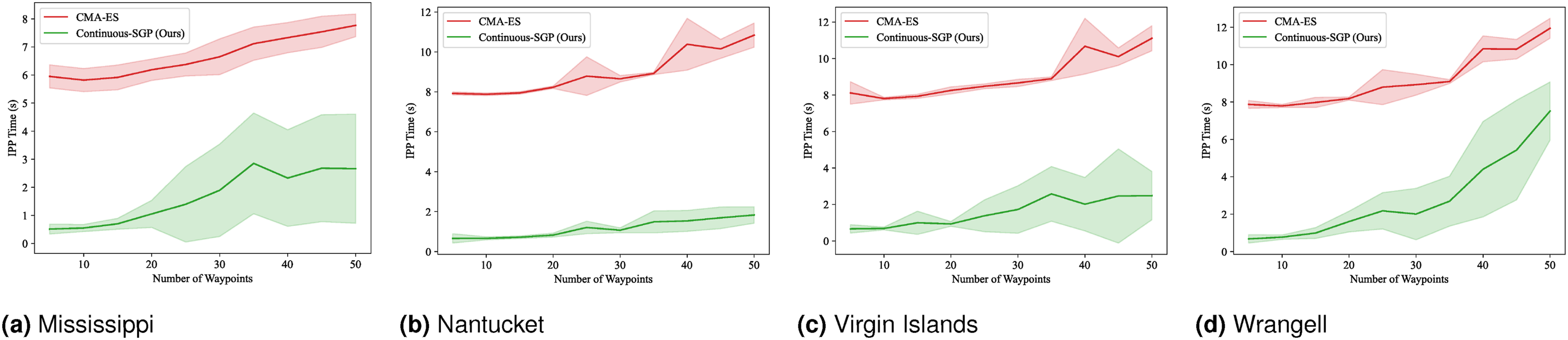
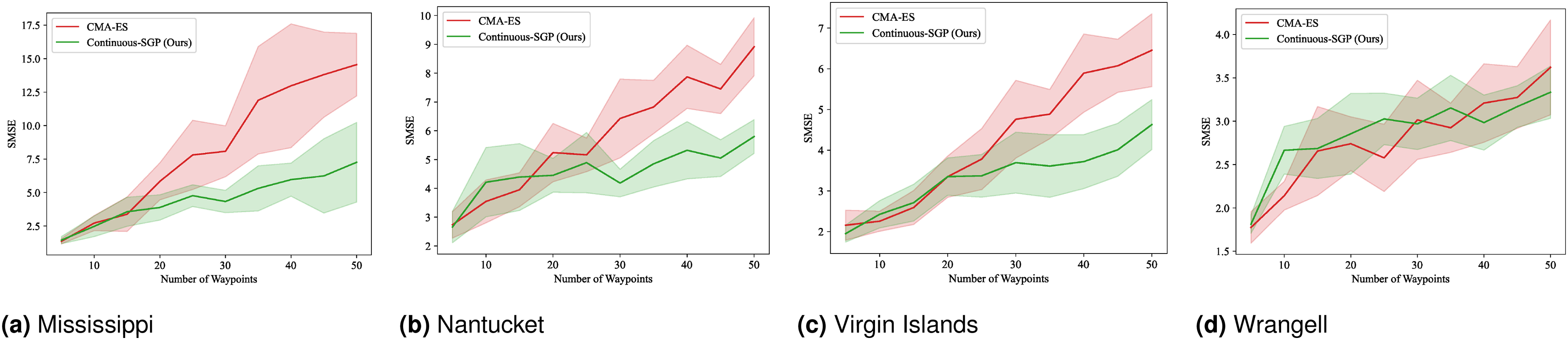
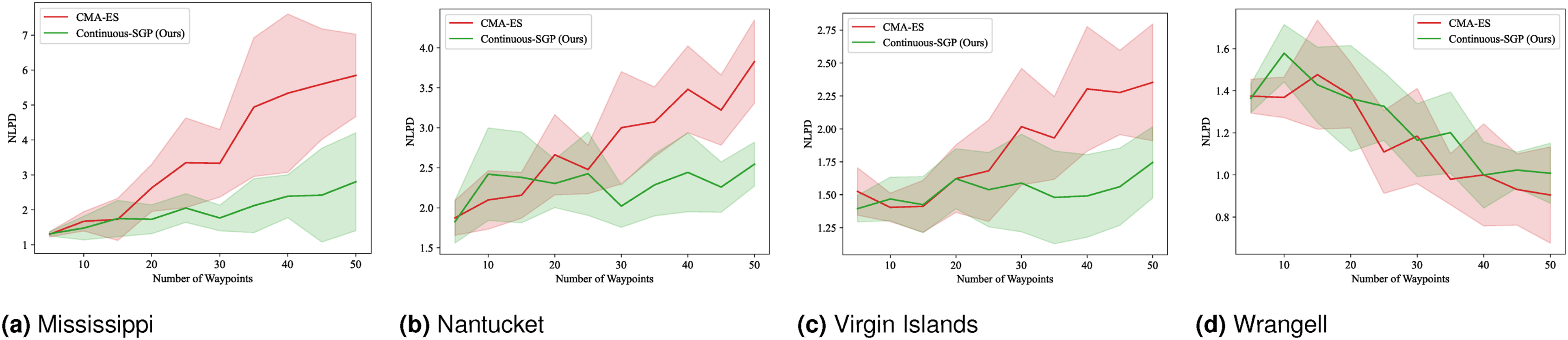
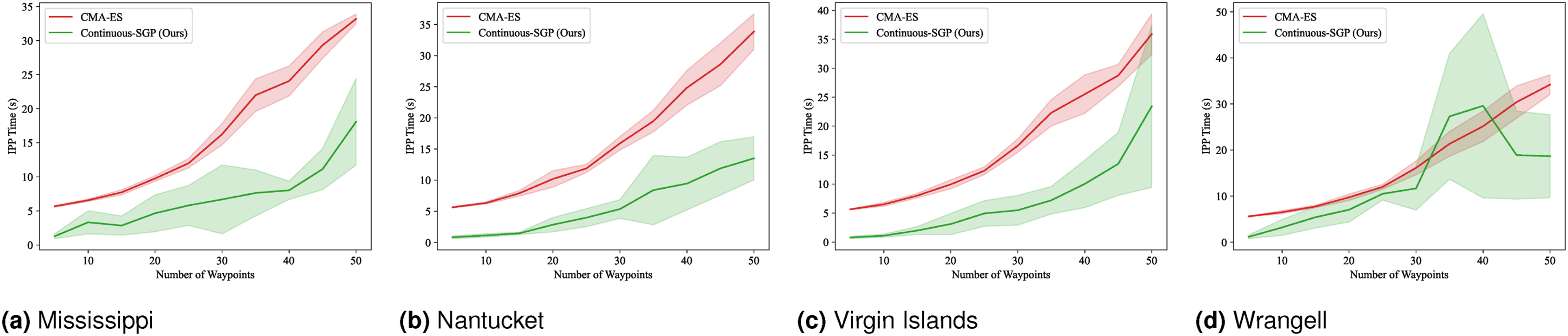
We computed the solution for 5 to 100 sensing locations in increments of 5. The mean and standard deviation of the evaluation metrics and runtime results are shown in Figures 4–7. RMSE results for SP: Mean and standard deviation of RMSE versus the number of waypoints. Lower values indicate better performance. SMSE results for SP: Mean and standard deviation of SMSE versus the number of waypoints. Lower values indicate better performance. NLPD results for SP: Mean and standard deviation of NLPD versus the number of waypoints. Lower values indicate better performance. Runtime results for SP: Mean and standard deviation of runtime versus the number of waypoints. Lower values indicate better performance. Note that the runtime for Discrete-SGP (blue) coincides with Continuous-SGP (green).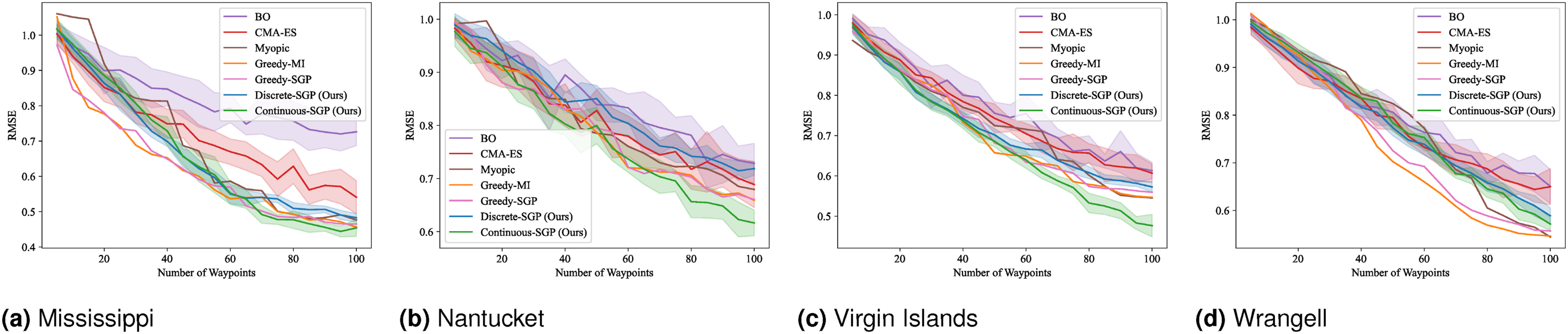
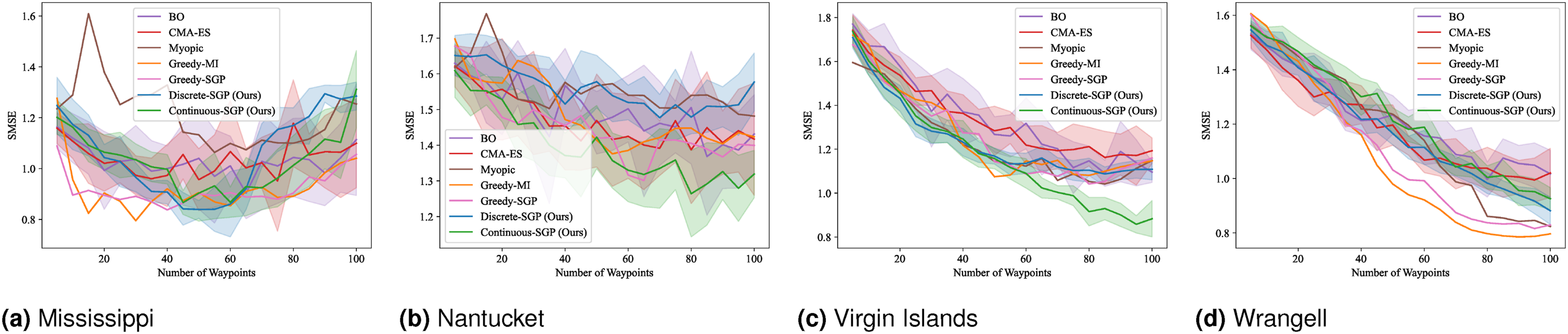
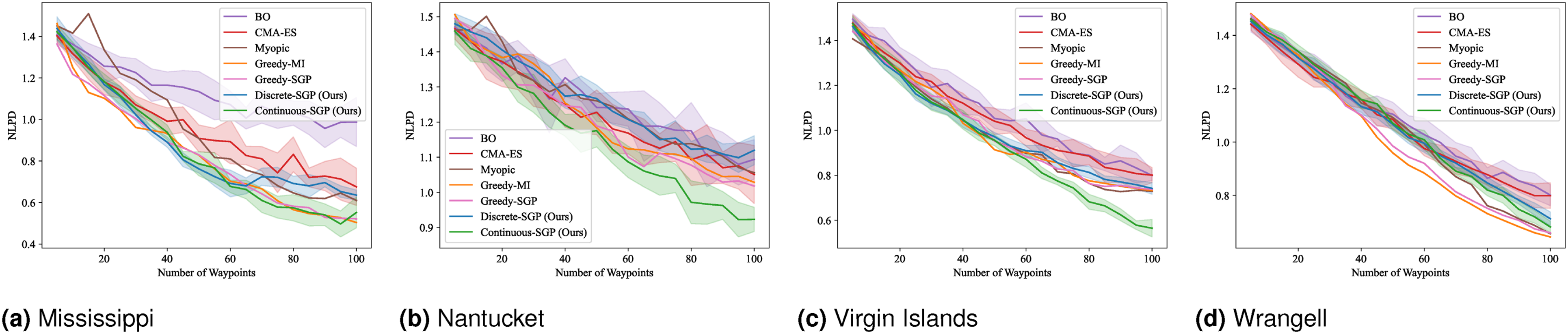
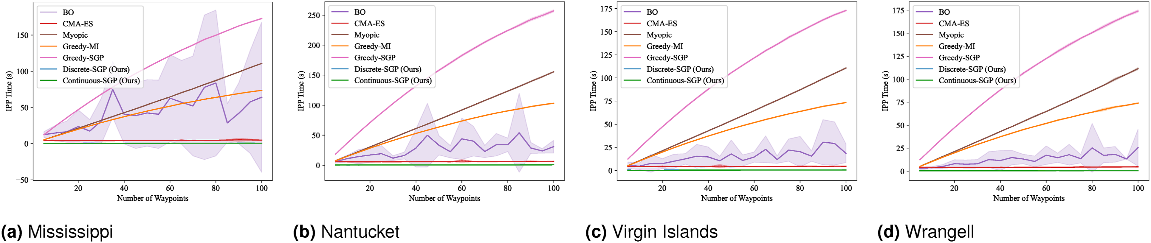
In terms of RMSE, SMSE, and NLPD, Continuous-SGP performs well in four datasets, with Discrete-SGP closely matching its performance in the discrete space. In terms of runtime, Continuous-SGP and Discrete-SGP (runtime coincident with Continuous-SGP in the plots) dominates every baseline approach. Indeed, compared to the next fastest method—CMA-ES, Continuous-SGP is on average 11.53, 12.5, 12.58, and 12.08 times faster on the Mississippi, Nantucket, Virgin Islands, and Wrangell datasets, respectively.
We attribute the fast runtime performance of Continuous-SGP to its computationally efficient optimization objective (Equation (11)) and its use of gradient-based optimization approach—conjugate gradient descent. The experiment also demonstrates that from a data field reconstruction accuracy perspective, Continuous-SGP is capable of performing on par or better then all considered baselines.
(Benchmark 2) Mutual information’s sensitivity to the number of candidate locations: A critical factor influencing the computational burden and estimation accuracy of mutual information (MI), Number of candidate locations benchmark results: Mean and standard deviation of RMSE, SMSE, NLPD, and runtime versus the number of waypoints. Lower values indicate better performance. For CMA-ES, the number of candidates was varied, while Continuous-SGP consistently used 2500 candidates. Note that the performance of Continuous-SGP varies since the set of 2500 candidates is randomly sampled for each run.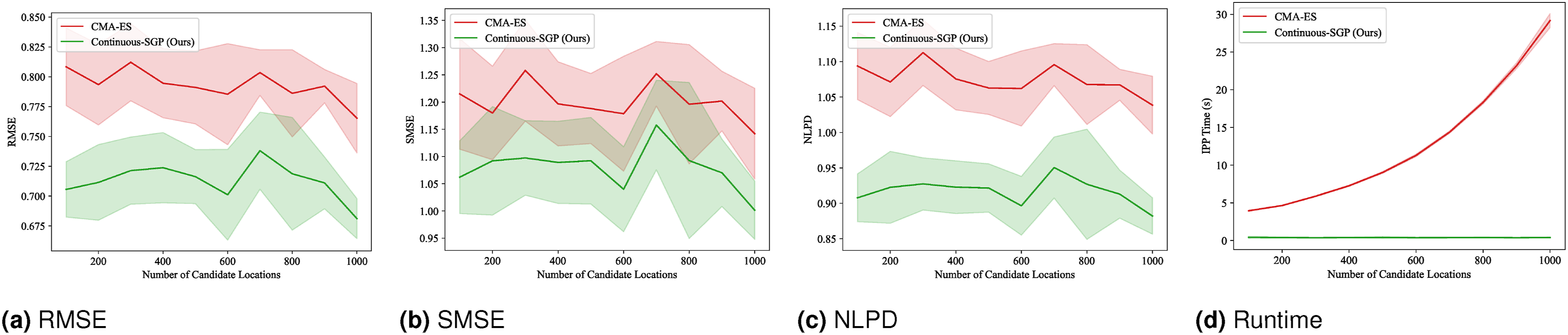
Our investigation into MI-based optimization revealed a significant increase in computational cost directly proportional to the number of candidate solutions considered. Despite this, higher MI resolution, achieved by increasing candidate density, did not yield a notable improvement in reconstruction quality for the CMA-ES algorithm on the specific dataset used in this study. This observation highlights a critical challenge: determining the optimal MI resolution a priori remains an open question.
In contrast, the Continuous-SGP approach, while similarly affected by training set size in terms of performance, demonstrated superior computational efficiency. This inherent efficiency allows for the use of a relatively larger number of unlabeled random locations (candidates) during optimization without incurring prohibitive runtime penalties. Note that the performance of Continuous-SGP varies since the set of 2500 candidates is randomly sampled for every run.
(Benchmark 3) Gradient-based optimizers: Here, we benchmark various gradient-based optimizers for their effectiveness with the Continuous-SGP approach. This benchmark includes both first-order and quasi-Newton optimizers (Goodfellow et al., 2016; Nocedal and Wright, 2006): Conjugate Gradient (CG), Broyden–Fletcher–Goldfarb–Shanno (BFGS), Limited-memory BFGS (L-BFGS-B), Stochastic Gradient Descent (SGD), Adam, RMSprop, and Nadam. For this analysis, we used the Wrangell dataset and varied the number of waypoints from 5 to 100 in increments of 5.
Figure 9 displays the mean and standard deviation of the evaluation metrics and runtime results. With the exception of SGD, all optimizers achieve very similar RMSE, SMSE, and NLPD scores, along with comparable standard deviations. In terms of runtime, CG, L-BFGS-B, and BFGS consistently outperform SGD, Adam, RMSprop, and Nadam. Notably, CG and L-BFGS-B appear to perform slightly better than BFGS. Gradient-based optimizer benchmark results: Mean and standard deviation of RMSE, SMSE, NLPD, and runtime versus the number of waypoints. Lower values indicate better performance.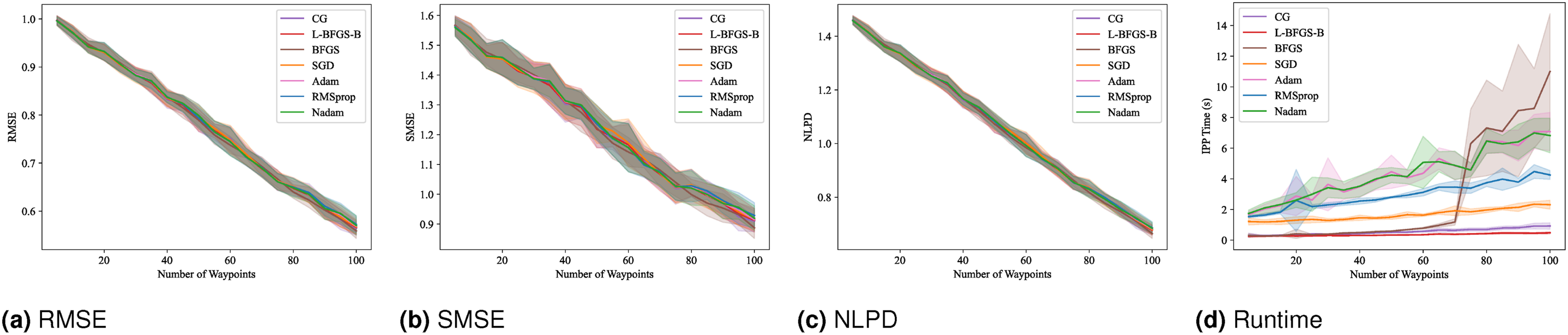
While quasi-Newton approaches are generally more computationally intensive per iteration, they often lead to faster convergence. Their scalability can be limited when the number of optimization parameters becomes exceptionally large. However, the Continuous-SGP approach involves a relatively small number of parameters compared to, for instance, deep learning models, which allows it to effectively leverage the benefits of quasi-Newton methods.
(Demonstration 1) Obstacle avoidance and non-point sensing: We handle obstacles in the environment by building an appropriate (zero-labeled) training dataset for the SGP. We remove the samples in the SGP training set at locations inside obstacles, resulting in a training set with samples only in obstacle-free regions. Training an SGP on such data would result in inducing points that avoid the obstacles since placing the inducing points at locations with obstacles would not increase the likelihood of the training data used to optimize the SGP. This obstacle avoidance approach is best suited for relatively large obstacles.
Figure 10 shows our SPs in an environment with multiple obstacles. Each sensor was modeled as a non-point sensor with a rectangular field-of-view (FoV) as detailed in Section Non-point field of view sensors. As we can see, the SPs avoid obstacles while accounting for the sensors’ non-point FoV. Sensor placements (100) generated using an SGP augmented with the expansion and aggregation transforms for sensors with a rectangular FoV. The hatched orange polygons represent obstacles in the environment. Each rectangular array of blue points represents the sensor’s FoV.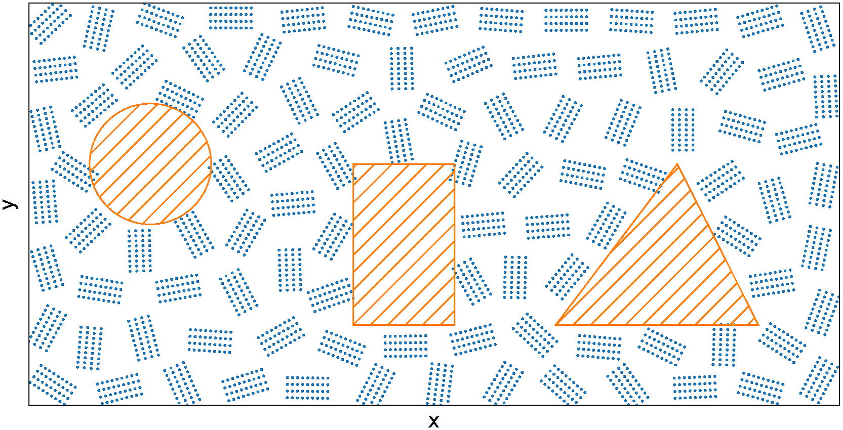
(Benchmark 4) Sensor placement in a non-stationary environment: When using stationary kernels, the SP solutions in the previous two experiments appear uniformly distributed. This reflects a key strength of GP-based methods: they can adapt the density of sensing locations to account for environmental boundaries and obstacles, while still producing evenly spaced placements in homogeneous fields. This property holds for both MI-maximizing approaches (Hitz et al., 2017; Krause et al., 2008) and our SGP method. In cases where the ideal sensing density is already known and no obstacles are present, faster uniform sampling strategies, such as Latin hypercube sampling (McKay et al., 1979), could achieve similar results.
We now consider non-stationary environments, in which the optimal sensing density varies spatially because the data field changes at different rates in different regions. For this experiment, we generated a synthetic non-stationary elevation field in which the left half varies at low frequency and the right half at higher frequency (Figure 11). The first row of Figure 12 shows results from the SGP method with a stationary RBF kernel (Rasmussen and Williams, 2005), which performs poorly in reconstructing the ground truth. Non-stationary environment elevation data. Estimates of a non-stationary environment generated using the continuous-SGP solutions with a stationary RBF kernel, non-stationary attentive kernel, and non-stationary neural kernel. The black pentagons represent the solution placements. The heat map displays elevation data (blue indicates low elevation, and red indicates high elevation).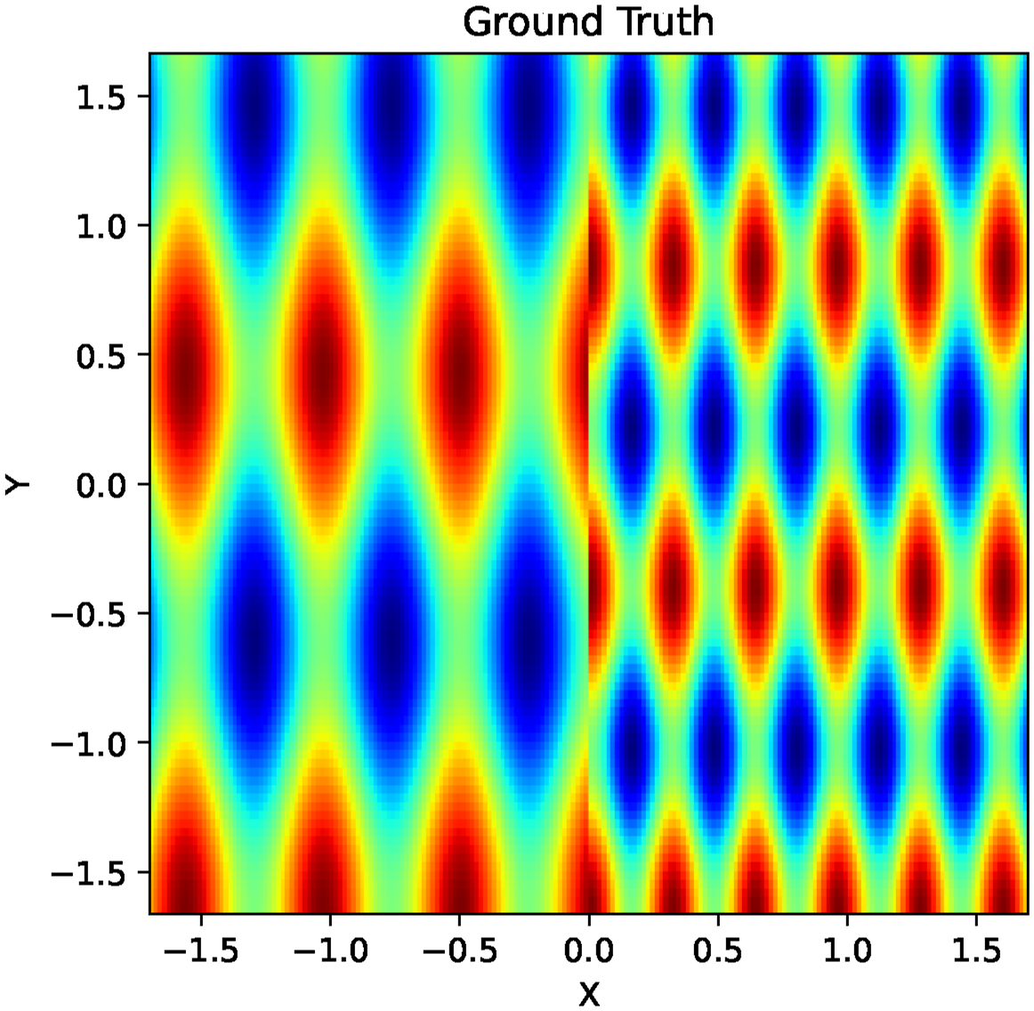
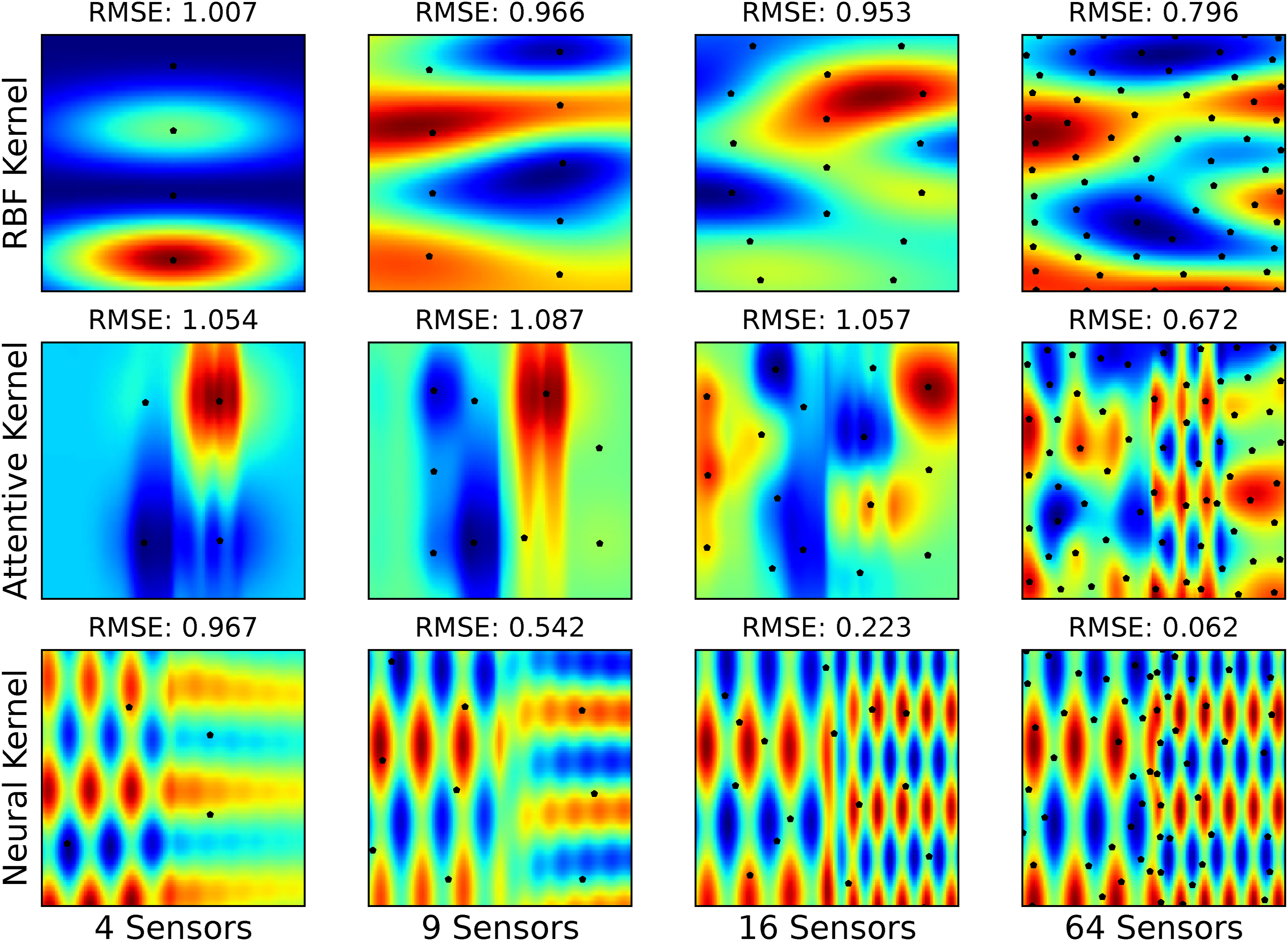
To address this, we evaluated two non-stationary kernels: the attentive kernel (Chen et al., 2022) and the neural kernel (Remes et al., 2018). The attentive kernel used 10 mixture component weights evenly spaced between 0.05 and 2.0, with a two-layer multilayer perceptron (Bishop, 2006) of 10 hidden units for mixture weight estimation. The neural kernel employed three mixture components, each parameterized by a two-layer multilayer perceptron with four hidden units. Both kernels were trained on 800 grid-sampled points from the environment using SGP optimization via type-II maximum likelihood (Bishop, 2006).
As shown in Figure 12, the resulting sensor placements are no longer uniform but instead concentrate in regions critical for accurate reconstruction. The attentive kernel performs poorly with 16 or fewer sensors but produces strong reconstructions when the number of sensors increases (e.g., 64). The neural kernel consistently yields the lowest RMSE scores and, in this particular test case, achieves near-perfect reconstruction with 64 sensors. It is important to note, however, that this exceptional performance is context-dependent: the ground-truth field used here is well aligned with the spectral mixture prior embedded in the neural kernel, and such results are generally achievable only when the prior strongly matches the underlying field structure or when the environment exhibits high regularity. In less structured or mismatched settings, achieving comparable accuracy with so few sensors would be challenging.
Informative path planning
This section evaluates the performance of our IPP approach across various scenarios. We assess its effectiveness in single-robot and multi-robot settings, incorporating both discrete and continuous sensing models with distance budget constraints. We also evaluate the performance of multiple gradient-based optimizers to optimize our IPP approach. We further demonstrate the adaptability of our IPP method in spatiotemporal and 3D environments, employing a non-point sensing model.
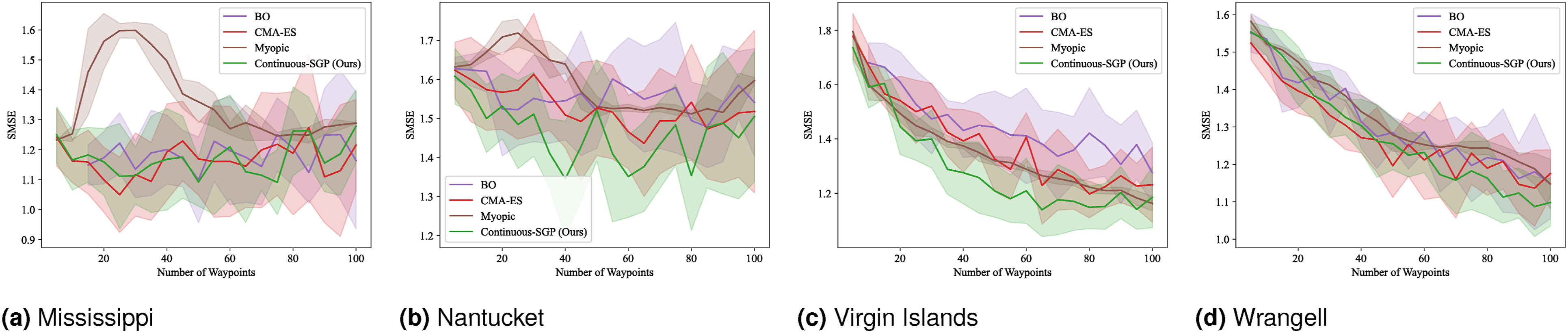
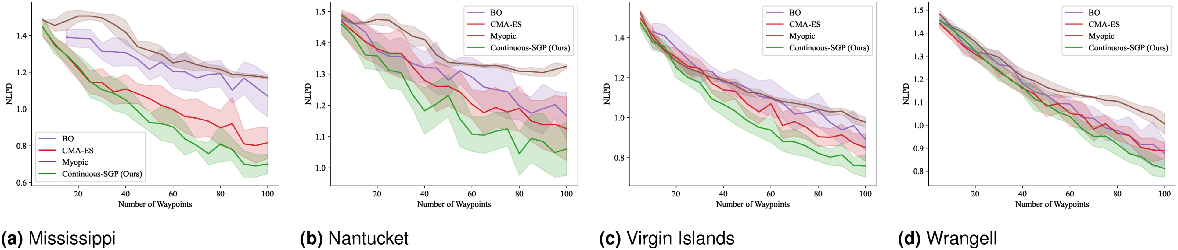
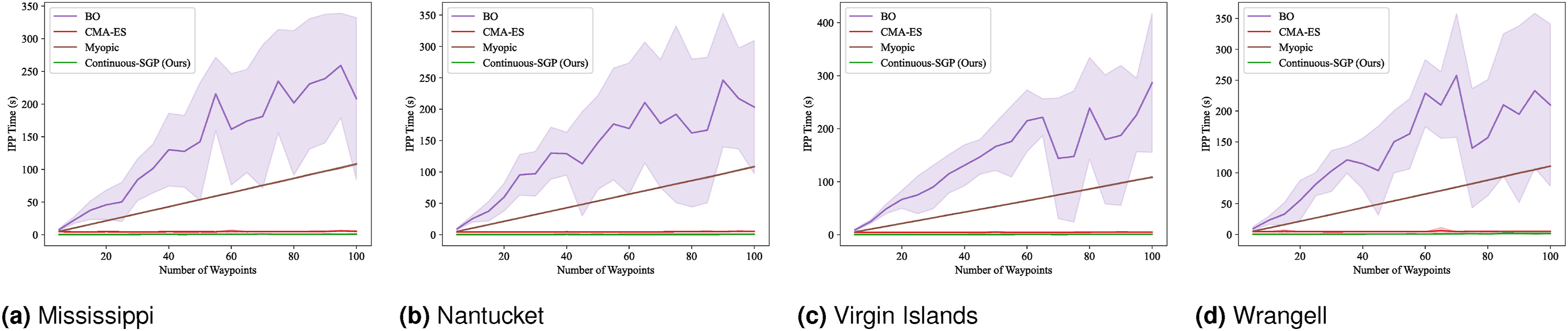
(Benchmark 5) Single robot IPP with distance budget: This benchmark evaluates our Continuous-SGP approach against several baselines in a single-robot IPP scenario with a distance budget and a discrete sensing model. Continuous-SGP (Section Single-robot IPP) optimizes the objective function (Equation (11)) using L-BFGS-B optimizer to determine optimal sensing locations. The distance constraint (Equation (17)) is integrated into the objective function via a weighted penalty term. We compare Continuous-SGP with three established baseline approaches: Bayesian optimization (BO), covariance matrix adaptation evolution strategy (CMA-ES), and a Myopic strategy, all of which inherently support distance constraints.
We generated IPP solutions for paths with the number of waypoints ranging from 5 to 100, in increments of 5. The distance budget was dynamically set to the length of the initial path minus 5 m. This dynamic adjustment ensures that the budget remains relevant to the path length, avoiding scenarios where it is either too restrictive or excessively generous.
Figures 13–16 present the mean and standard deviation for the evaluation metrics (RMSE, SMSE, NLPD) and runtime results, respectively. Across all metrics, Continuous-SGP consistently performs on par with or better than the baselines. Critically, it achieves these performance levels with significantly faster execution times. Specifically, Continuous-SGP is, on average, 8.31, 11.31, 9.87, and 6.40 times faster than the next fastest baseline on the Mississippi, Nantucket, Virgin Islands, and Wrangell datasets, respectively. This highlights the computational efficiency of our approach. RMSE results for single-robot IPP with a distance budget: Mean and standard deviation of RMSE versus the number of waypoints. Lower values indicate better performance. SMSE results for single-robot IPP with a distance budget: Mean and standard deviation of SMSE versus the number of waypoints. Lower values indicate better performance. NLPD results for single-robot IPP with a distance budget: Mean and standard deviation of NLPD versus the number of waypoints. Lower values indicate better performance. Runtime results for single-robot IPP with a distance budget: Mean and standard deviation of runtime versus the number of waypoints. Lower values indicate better performance.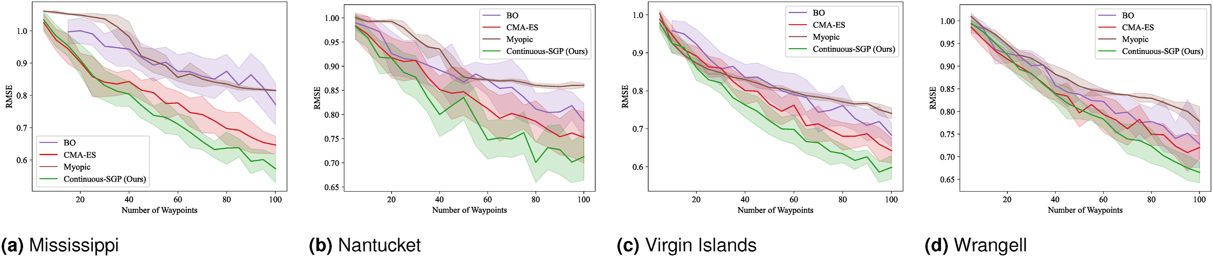
(Benchmark 6) Single-robot IPP with a distance budget and continuous sensing model: The previous benchmark assumed a discrete sensing robot, where sensing occurs only at the waypoints. However, many real-world sensors, such as sonars and lidars, operate continuously along a robot’s path. This benchmark evaluates the performance of IPP approaches for a continuous sensing robot.
In addition to Continuous-SGP, we include BO and CMA-ES as baselines. These baselines were chosen because our transform-based approach (Section Continuous sensing robots) can be effectively integrated with them to account for information gathered continuously along the entire path.
The mean and standard deviation of the evaluation metrics and runtime results are presented in Figures 17–20. Consistent with the discrete sensing scenario, Continuous-SGP once again demonstrates performance on par with or better than the baselines in terms of RMSE, SMSE, and NLPD, while maintaining a significant speed advantage. RMSE results for single-robot IPP with a distance budget and continuous sensing model: Mean and standard deviation of RMSE versus the number of waypoints. Lower values indicate better performance. SMSE results for single-robot IPP with a distance budget and continuous sensing model: Mean and standard deviation of SMSE versus the number of waypoints. Lower values indicate better performance. NLPD results for single-robot IPP with a distance budget and continuous sensing model: Mean and standard deviation of NLPD versus the number of waypoints. Lower values indicate better performance. Runtime results for single-robot IPP with a distance budget and continuous sensing model: Mean and standard deviation of runtime versus the number of waypoints. Lower values indicate better performance.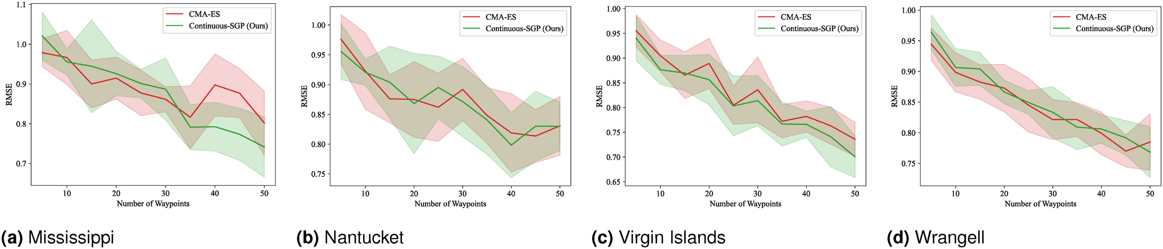
(Benchmark 7) Multi-robot IPP with distance budgets: This benchmark extends our evaluation to multi-robot (four robots) IPP scenarios, incorporating distance budget constraints and a discrete sensing model. We generated solutions for paths with waypoint counts ranging from 5 to 50, in increments of 5. For this multi-robot setting, CMA-ES was selected as the primary baseline due to its support for multi-robot IPP.
Figures 21–24 display the mean and standard deviation of the evaluation metrics and runtime results. The RMSE, SMSE, and NLPD plots are consistent with our single-robot findings, indicating that Continuous-SGP performs comparably to or better than CMA-ES. The runtime plots are particularly noteworthy, clearly illustrating the significant performance difference between the two methods, with Continuous-SGP being at least six times faster than CMA-ES on average. RMSE results for multi-robot IPP (four robots) with a distance budget: Mean and standard deviation of RMSE versus the number of waypoints. Lower values indicate better performance. SMSE results for multi-robot IPP (four robots) with a distance budget: Mean and standard deviation of SMSE versus the number of waypoints. Lower values indicate better performance. NLPD results for multi-robot IPP (four robots) with a distance budget: Mean and standard deviation of NLPD versus the number of waypoints. Lower values indicate better performance. Runtime results for multi-robot IPP (four robots) with a distance budget: Mean and standard deviation of runtime versus the number of waypoints. Lower values indicate better performance.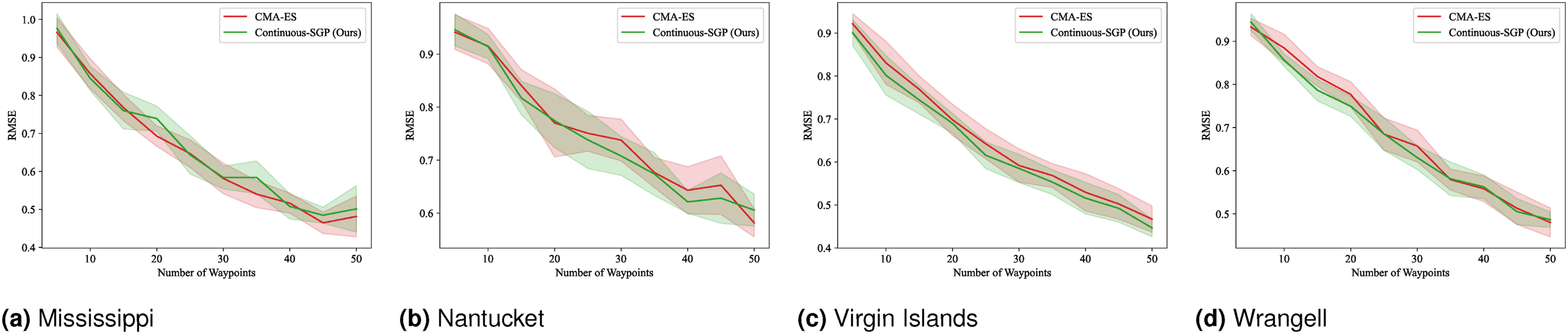
(Benchmark 8) Multi-robot IPP with distance budgets and continuous sensing: This experiment repeats the multi-robot IPP evaluation, but now incorporating a continuous sensing model. The mean and standard deviation for the evaluation metrics and runtime are shown in Figures 25–28. RMSE results for multi-robot IPP (four robots) with a distance budget and continuous sensing model: Mean and standard deviation of RMSE versus the number of waypoints. Lower values indicate better performance. SMSE results for multi-robot IPP (four robots) with a distance budget and continuous sensing model: Mean and standard deviation of SMSE versus the number of waypoints. Lower values indicate better performance. NLPD results for multi-robot IPP (four robots) with a distance budget and continuous sensing model: Mean and standard deviation of NLPD versus the number of waypoints. Lower values indicate better performance. Runtime results for multi-robot IPP (four robots) with a distance budget and continuous sensing model: Mean and standard deviation of runtime versus the number of waypoints. Lower values indicate better performance.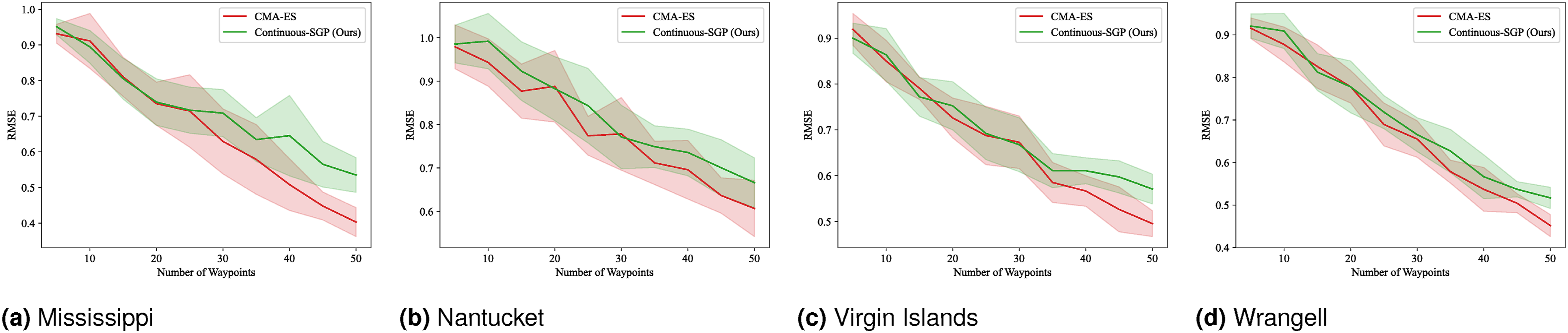
The results from this benchmark are particularly insightful. While generally consistent with previous benchmarks—demonstrating that Continuous-SGP is on par with or better than the baseline and considerably faster—we observe instances where Continuous-SGP takes longer to converge to a solution. We hypothesize that the added complexity of multi-robot settings combined with path constraints leads to a more intricate optimization landscape, which can sometimes slow down convergence.
Despite this increased complexity, Continuous-SGP consistently finds a better solution in terms of RMSE, SMSE, and NLPD compared to the baseline in most cases. To further improve runtime in such challenging scenarios, several approaches could be explored: • Early stopping techniques (Bishop, 2006) could be employed to identify when the solution has sufficiently converged, preventing unnecessary computation. • Improved sampling techniques for initial sensing locations (Bauer et al., 2016) could lead to faster and more informative initial solutions. • The quality of the initial path(s) generated by the traveling salesperson problem (TSP) or vehicle routing problem (VRP) solver plays a critical role in multi-robot scenarios. While we currently use an approximate solver, employing an exact solver or dedicating more computational time to obtain a superior initial path could significantly reduce the overall IPP runtime.
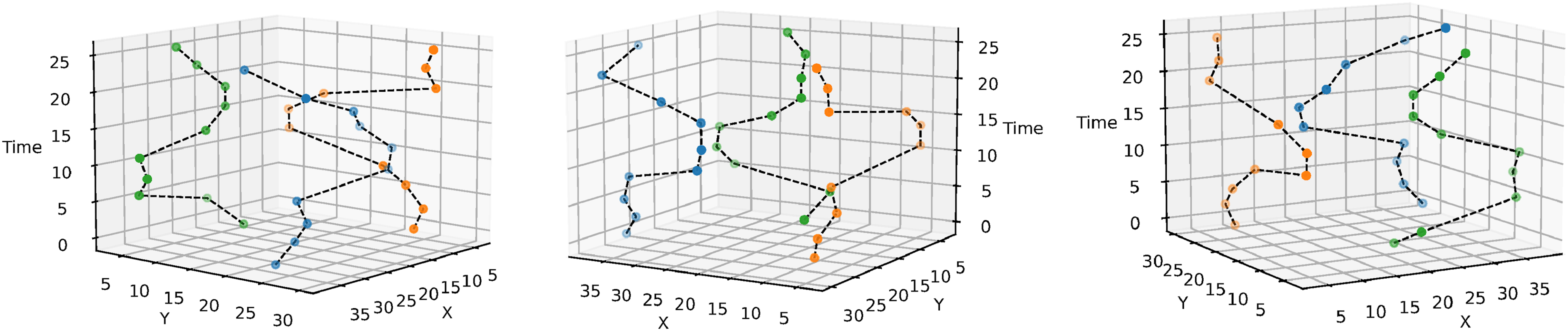
(Demonstration 2) IPP in a spatiotemporal environment: Next, we demonstrate our approach for IPP with a distance constraint in a spatiotemporal environment. A GP was used to sample dense spatiotemporal synthetic temperature data. We used an RBF kernel with a length scale of 7.70 m, 19.46 m, and 50.63 minutes along the x, y, and temporal dimensions, respectively. We generated paths by optimizing the inducing points with the SGP approach with distance budgets of 10 m, 20 m, and 40 m. The results are shown in Figure 29. Our approach consistently uses the total distance budget without exceeding it to get the maximum amount of new data, as evident from the paths’ RMSE scores. We also show the paths generated for three robots in the same environment with a distance budget of 50 m for each robot (Figure 30). Single-robot IPP solution paths generated using a spatiotemporal kernel function for different distance budgets. X and Y axes are in meters, and the time axis is in minutes. Three different views of our multi-robot IPP solution paths for a spatiotemporal data field with a distance budget of 50 m for each robot. The solution path lengths were 47.29 m (blue), 47.44 m (orange), and 47.20 m (green) for the three robots. The total RMSE was 2.75. X and Y axes are in meters, and the time axis is in minutes.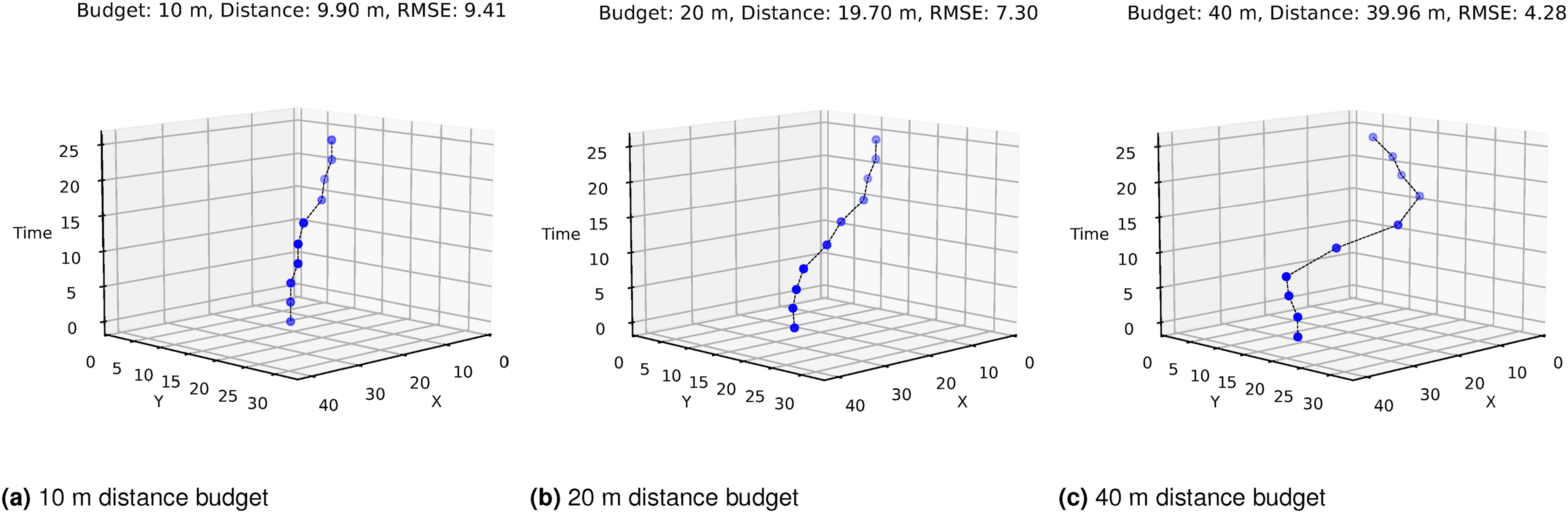
(Demonstration 3) IPP in a 3D environment with non-point sensing: Now, we demonstrate our approach in a 3D environment with a complex non-point sensing model. We can leverage the differentiability of SGPs to parameterize the inducing points and, by extension, the solution path in higher dimensions than the data field being monitored (Section Non-point field of view sensors). We do this by modeling a robot that operates in 3D space with a non-point sensor that behaves similarly to a camera, that is, the FoV area scales in proportion to the height from the ground. The data field was synthetically generated elevation data defined on a 2D plane. We then solved the IPP problem using our SGP approach. We used 16 auxiliary inducing points to approximate each sensor’s FoV area, and the spacing between the auxiliary inducing points was adjusted in proportion to the height from the ground to approximate the 2D FoV area. The path was modeled with a discrete sensing model, that is, the robot senses at the path’s vertices. Please refer to our code for additional details of the experiments presented in this section. Figure 31 shows our solutions for paths with different numbers of sensing waypoints. As we can see, our approach optimized the waypoints in 3D space to simultaneously ensure complete coverage of the environment and good ground sampling resolution. Solution paths for a discrete sensing robot with a square height-dependent FoV area sensor. The sensing height is optimized to balance the ground sampling resolution and the FoV area (black squares).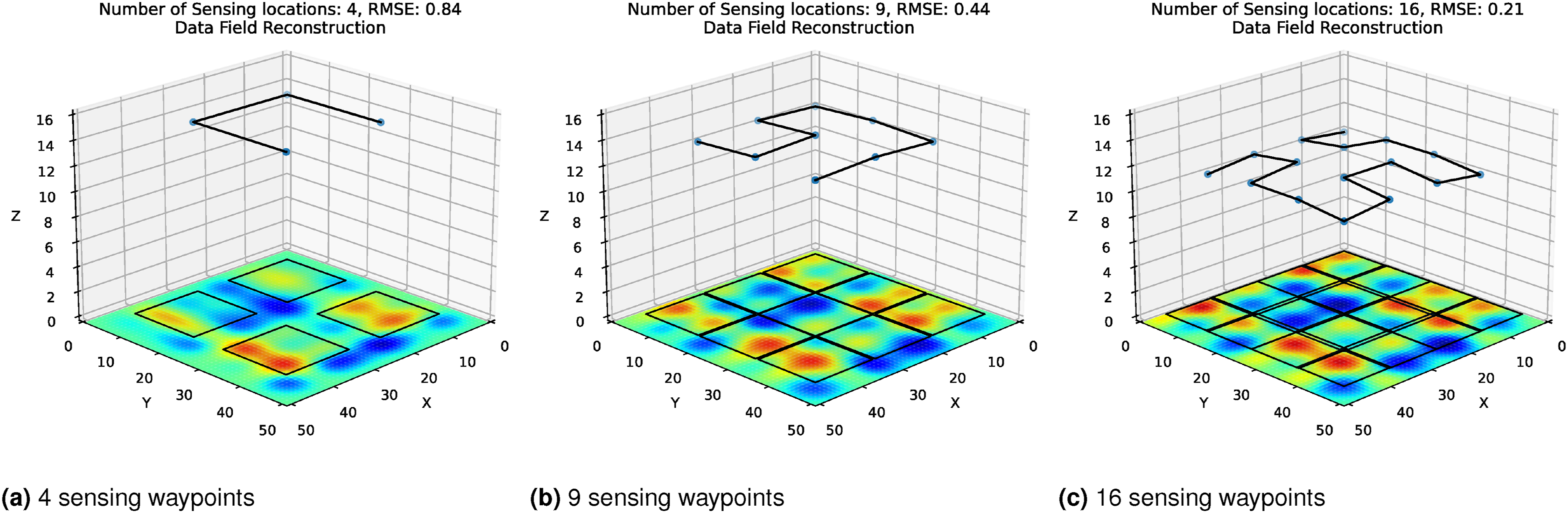
(Benchmark 9) IPP in a non-stationary environment: Finally, we demonstrate the IPP approach in a non-stationary environment using Shuttle Radar Topography Mission (SRTM) elevation data (NASA JPL, 2013) as the ground truth field (Figure 32, first column). Ground truth non-stationary SRTM elevation data and estimates generated using the SGP-IPP solutions with a stationary RBF kernel, non-stationary attentive kernel, and non-stationary neural kernel. The dotted red paths represent the solution paths. Note the X, Y, and Z axes are in normalized units.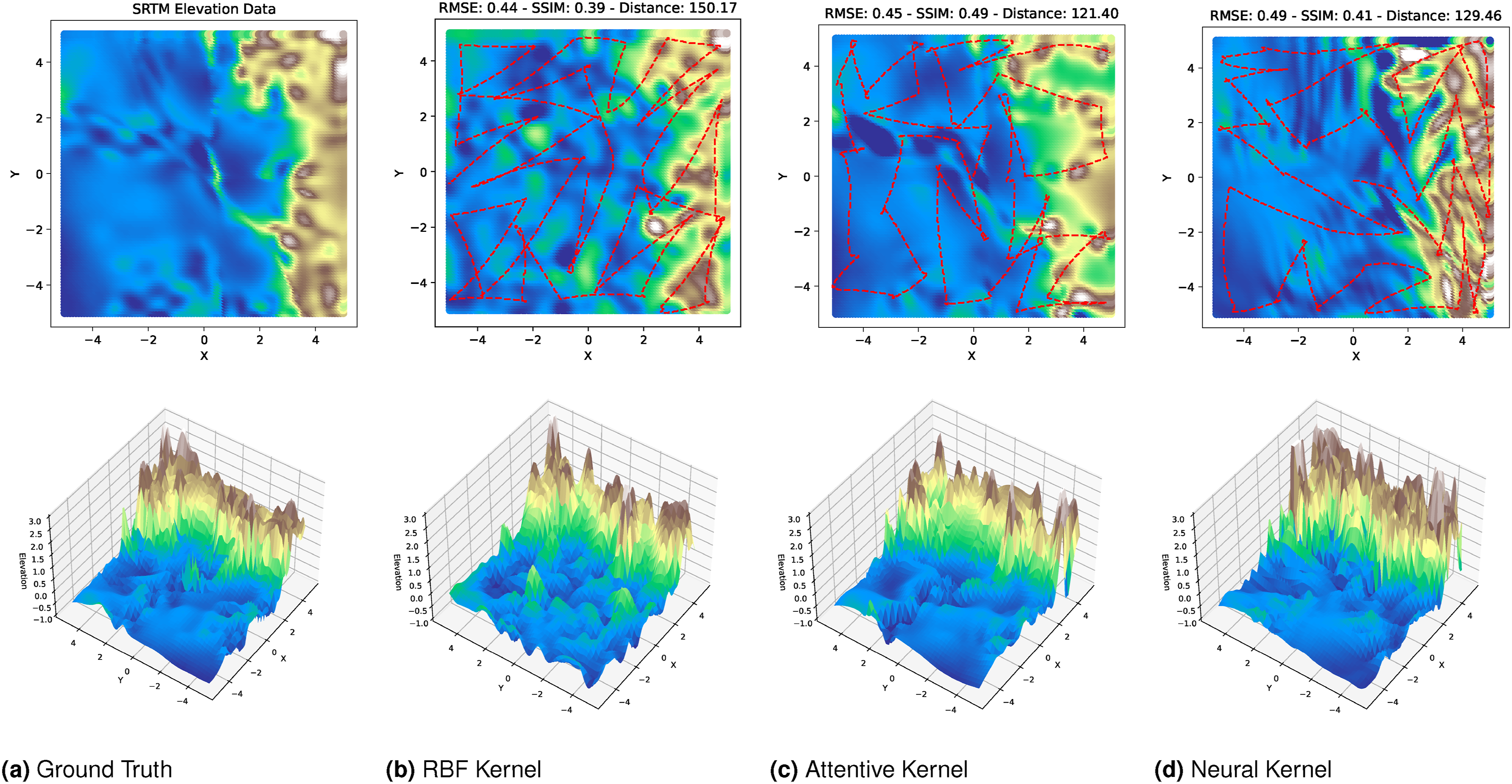
We first collected training data via an initial lawn mower path and used it to optimize kernel parameters. Three kernel functions were considered: RBF (Rasmussen and Williams, 2005), attentive (Chen et al., 2022), and neural (Remes et al., 2018). The attentive kernel employed 10 mixture component weights evenly spaced between 0.1 and 2.5, with a two-layer multilayer perceptron (Bishop, 2006) of 10 hidden units for weight estimation. The neural kernel used five mixture components, each with a two-layer multilayer perceptron containing four hidden units. Parameters for all kernels were learned with a sparse Gaussian process (SGP) via type-II maximum likelihood (Bishop, 2006).
We applied the SGP-IPP method with a continuous sensing model and a sampling rate of 5, optimizing for 40 waypoints. The second, third, and fourth columns of Figure 32 show the reconstruction results, along with RMSE, SSIM (Wang et al., 2004), and the resulting path lengths.
In terms of RMSE and SSIM, the RBF-based approach achieves the best scores. This outcome is consistent with known trade-offs in non-stationary kernel methods: non-stationary kernels, while more expressive, often require substantial training data to learn robust spatially varying length-scales. As a result, their initial performance under sparse data regimes may match or even lag behind simpler stationary kernels, as discussed in recent work on efficient training strategies for non-stationary kernels, such as Probabilistic Online Attentive Mapping (POAM) (Chen et al., 2024).
When examining path lengths, however, the attentive and neural kernel approaches perform competitively while producing shorter paths. Moreover, despite its lower RMSE/SSIM performance, the RBF-based reconstruction fails to capture the relatively flat region on the left side of the field—an area that both non-stationary kernels successfully recover—highlighting their ability to model local variations that stationary kernels inherently cannot.
Field experiments
Our field experiments were conducted in two distinct environments to evaluate the performance of our informative path planning (IPP) method under real-world conditions. These experiments utilized a custom-built autonomous surface vehicle (ASV) and an Aqua2 autonomous underwater vehicle (AUV).
ASV experiments: Hechenbleikner Lake, Charlotte, NC, US. The first set of experiments was performed in Hechenbleikner Lake, Charlotte, NC, US, using a custom ASV developed by Brancato and Wolek (2024) (Figure 1). This environment was chosen due to its relatively static conditions, providing a controlled setting to assess the fundamental performance of the IPP method.
Vehicle and sensor configuration: The ASV was equipped with a Raspberry Pi 5 as its main computing unit. A downward-facing single-beam Ping sonar was used for mapping underwater bathymetry, and positioning data was provided by an onboard GPS.
IPP implementation and parameters: We deployed our IPP approach using both discrete and continuous sensing models, each configured with 20 waypoints. For the continuous sensing model, a sampling rate of five points per edge was employed to approximate the sonar’s continuous sensing along the path. The L-BFGS-B optimizer was used for on-board optimization and execution of the IPP solutions. We conducted an initial lawn mower mission to get ground truth data and determine the hyperparameters for the IPP approach, that is, the kernel parameters and data likelihood. Figure 33 shows the ground truth bathymetry data, reconstructed from the initial lawn mower mission. Red lines indicate the data collection locations. An RBF kernel function was used for these experiments. Note that the vehicle always collects data continuously along the path, regardless of whether a discrete or continuous sensing model was used to represent the sensor in the IPP approach. Ground truth bathymetry of Hechenbleikner lake estimated from data collected using the ASV while traversing a lawn mower path. The red lines represent the locations where the data was collected by the ASV.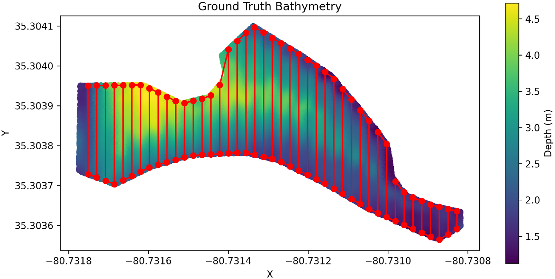
Results and analysis: Figure 34 shows bathymetry reconstructions and prediction variance generated from data collected by the ASV while executing the IPP solutions. The root mean square error (RMSE), standardized mean square error (SMSE), and negative log probability density (NLPD) are reported, comparing the reconstructions from the IPP missions to the ground truth lawn mower mission. Estimated bathymetry and prediction variance computed using the data collected by the ASV from executing the IPP solutions. The red points represent the locations where the data was collected by the ASV.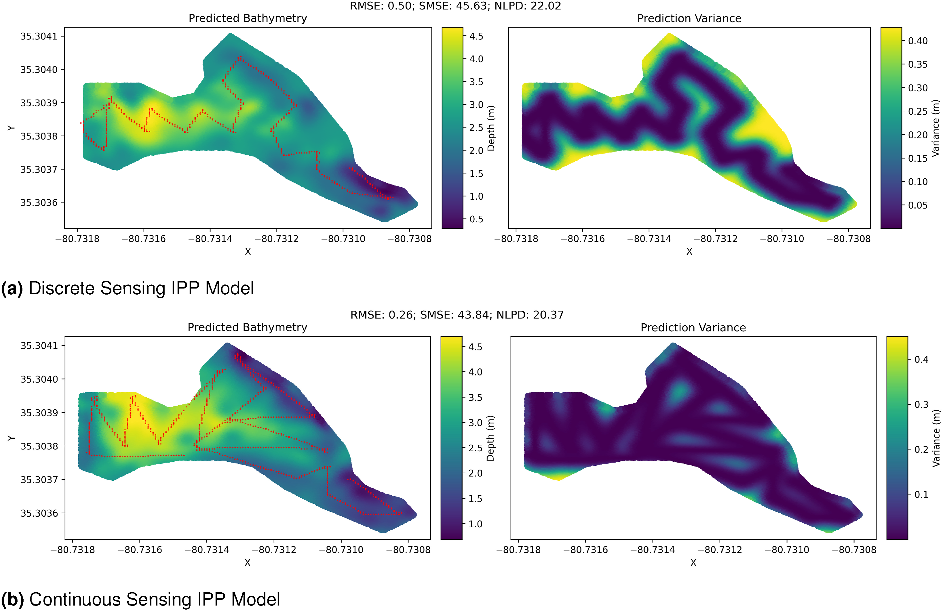
Both the discrete and continuous sensing approaches yielded good reconstructions of the environment. The ASV’s single-beam sonar continuously senses depth along the entire path. The continuous sensing model within our IPP approach resulted in a longer solution path, which, in turn, achieved a demonstrably better reconstruction. This highlights the significant advantage of incorporating a continuous sensing model for robots equipped with continuous sensing capabilities in real-world scenarios.
AUV experiment: Folkestone Marine Reserve, Barbados. The second experiment took place in the Folkestone Marine Reserve, near the Bellairs Research Institute of McGill University in Barbados. This location, characterized by strong ocean currents, tides, and unknown underwater surface terrain, served as an ideal real-world environment to test the robustness and necessity of IPP. The Aqua2 AUV (Figure 35, Dudek et al. (2007)) was the primary platform for these experiments. Aqua2 autonomous underwater vehicle (AUV) in the Folkestone Marine Reserve.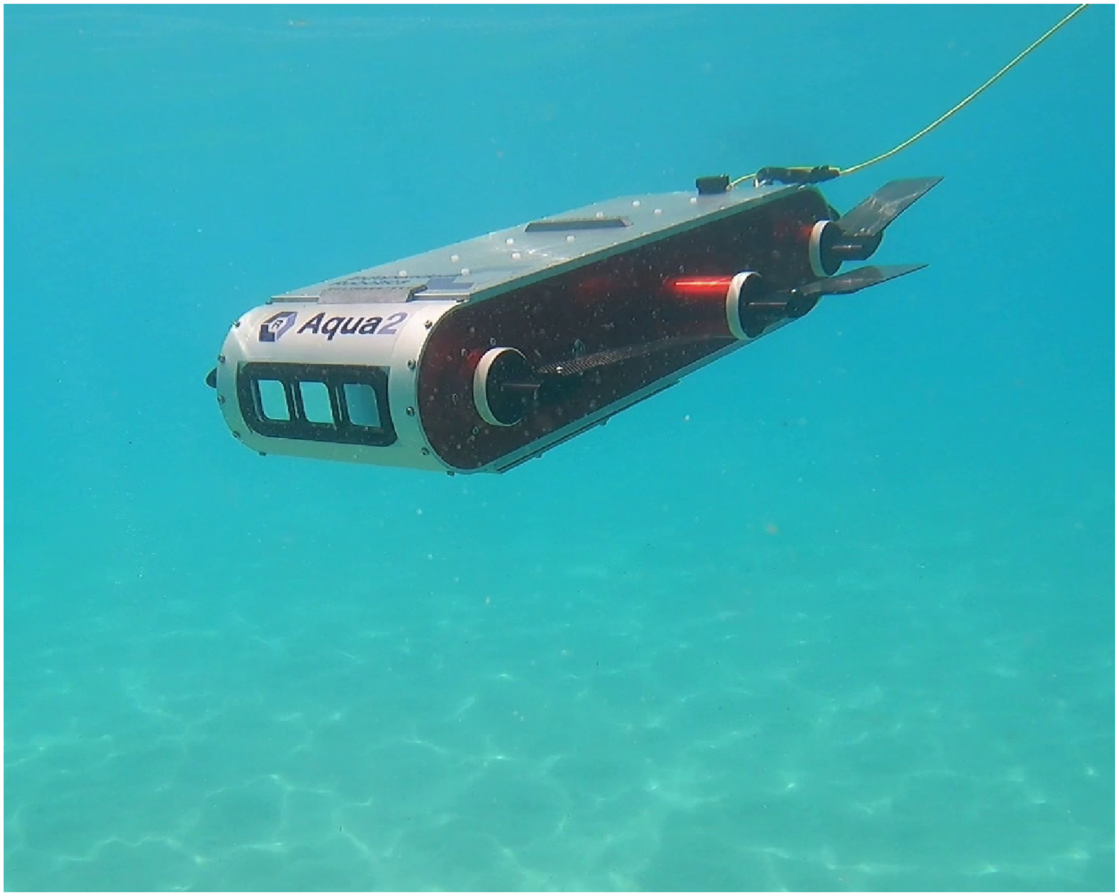
Vehicle and sensor configuration: The Aqua2 AUV utilized a downward-facing camera as its primary sensor for mapping the underwater surface. To mitigate the optical phenomena (attenuation and scattering) inherent in underwater imaging, the Osmosis deep-learning-based image correction method (Nathan et al. (2024)) was applied. This correction process, however, constrained the camera’s field of view (FoV) to a square shape. An onboard Doppler velocity logger (DVL) provided the vehicle’s positioning data.
IPP implementation and parameters: The Aqua2 was constrained to operate at a fixed depth of 1.5 m to prevent collisions with the underwater terrain. The IPP approach was configured to plan 20 waypoints using an RBF kernel and a discrete-sensing model. The choice of a discrete-sensing model was justified by the fixed, square-shaped FoV, which could be well approximated using an appropriate kernel lengthscale. In this experiment, a lengthscale of 0.1 m and a variance of 0.5 were used for the kernel.
Results and analysis: Figure 36(a) illustrates the planned and executed paths of the Aqua2. Figure 36(b) displays the corresponding 3D reconstruction generated from the collected images using WebODM (OpenDroneMap (2024)). It is important to note that the reconstruction appears incomplete, primarily because the reconstruction algorithm could not fully utilize all collected images, even after color correction. An AUV equipped with an imaging sonar would likely yield more complete reconstructions. (a) The planned path (blue dotted path) and executed path (orange path). We see that the IPP solution visits all regions in the environment. (b) 3D reconstruction generated from the images captured using the downward facing camera onboard the Aqua2. The images were color-corrected using a deep-learning-based model before reconstruction.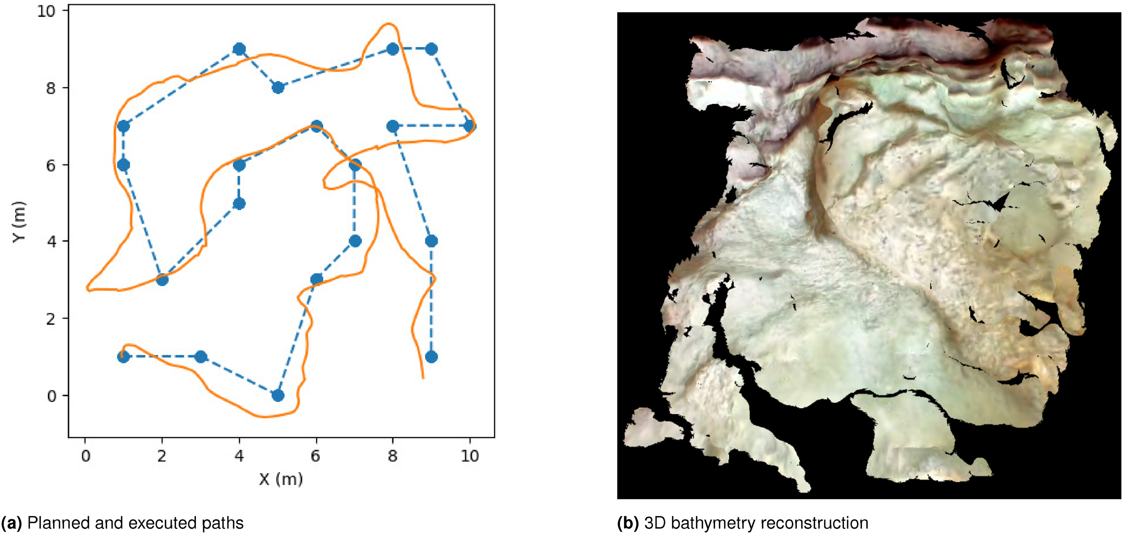
The IPP solution path uniformly covered all regions of the environment, thereby validating the efficacy of the IPP approach in achieving broad environmental coverage. The uniform coverage is largely attributable to the selection of a stationary RBF kernel function. For larger-scale missions, the use of non-stationary kernel functions could generate more informative paths that visit different regions non-uniformly, as demonstrated in Figure 32.
Challenges: Several challenges were encountered during the Aqua2 AUV experiment. The Aqua2 was unable to precisely follow the planned path, which can be attributed to multiple factors. First, the Aqua2 is a non-holonomic vehicle, and its motion constraints were not explicitly incorporated into the current IPP planner. Second, the Aqua2’s DVL, used for position tracking, is susceptible to errors when ocean currents and tides agitate underwater surface sand. Finally, the strong ocean currents and tides directly impacted the AUV’s trajectory, pushing it off course. These observations suggest promising avenues for future research, particularly in developing IPP methods that account for vehicle motion constraints and real-time localization uncertainty.
SGP-based IPP discussion
A natural question that our IPP work raises is when to use lawn mower paths and when to use our approach. We note that an implicit assumption in our work—and, by extension, in any approach that uses Gaussian process-based mutual information—is that the phenomenon being monitored is spatially and/or temporally correlated. We also assume knowledge of how the phenomenon is correlated.
If the underlying phenomenon is stationary, our solution paths would uniformly sample the entire environment and leverage the correlations to maximize the amount of information gathered by adjusting the data collection path (shortening or lengthening it) in response to how well the environment is correlated. In contrast, a naive lawn mower path would not account for such information and would use a fixed-length path.
Moreover, if the underlying phenomenon is non-stationary, our solution paths would sample the environment in a non-uniform manner, focusing on critical locations likely to provide the most information.
Finally, in addition to leveraging the correlations in the phenomenon, our formulation allows for the enforcement of novel constraints on the sensing locations and/or the solution path, as it is fully differentiable.
Limitations and future work
While our approach demonstrates substantial performance benefits, several limitations remain that point toward important avenues for future research.
First, in our multi-robot benchmarks, we occasionally observed slower convergence relative to the single-robot setting. Potential remedies include improved stopping criteria, more effective initialization of sensing locations, and higher-quality vehicle routing problem (VRP) solutions. Although these strategies are promising, their impact on convergence has not yet been rigorously benchmarked and represents a valuable direction for future study.
Second, the current multi-robot framework is implemented with a centralized planner. While sufficient for controlled experiments, a decentralized approach would be more robust and scalable in real-world deployments. Extending our differentiable framework to decentralized multi-robot IPP is therefore an important next step.
Finally, the methods presented here are situated within a semi-supervised IPP setting, in which prior data are required to learn kernel parameters before planning. This limitation is common to many semi-supervised IPP approaches. In our recent work on Adaptive IPP (Jakkala and Akella, 2025), we addressed this gap by extending the framework to handle streaming data and online model updates. That adaptive extension directly benchmarks against adaptive baselines and demonstrates superior performance relative to the semi-supervised variant described in this paper.
Related work
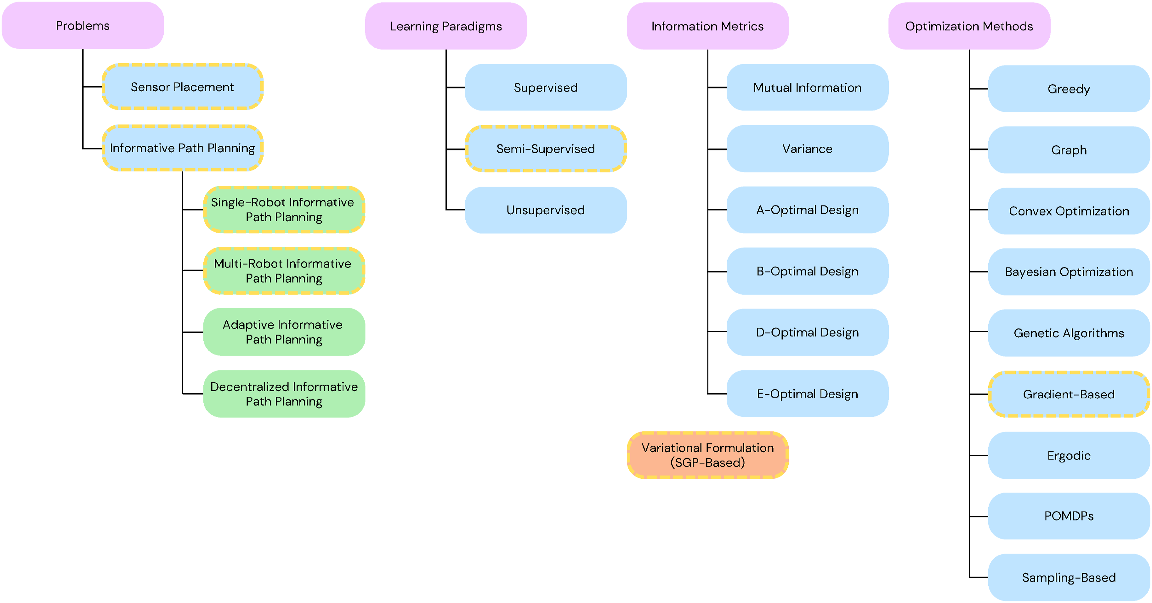
This work addresses the sensor placement (SP) and informative path planning (IPP) problems, both of which have been extensively studied in robotics, environmental monitoring, and related fields (Figure 37). While SP and IPP are distinct, they share significant conceptual overlap—many SP techniques have direct IPP analogs. Figure 38 presents a taxonomy of these problems, their variants, and common solution approaches. The methods developed in this article are highlighted in yellow, emphasizing our novel variational formulation for SP and IPP, which is distinct from conventional information-theoretic metrics. Illustration of autonomous vehicles monitoring an environment. A taxonomy of sensor placement and informative path planning problems, their variants, and solution approaches. The problems and methods presented in this article are outlined with a yellow dotted line. Note that our variational formulation for SP and IPP is a new approach that does not use any conventional information metrics.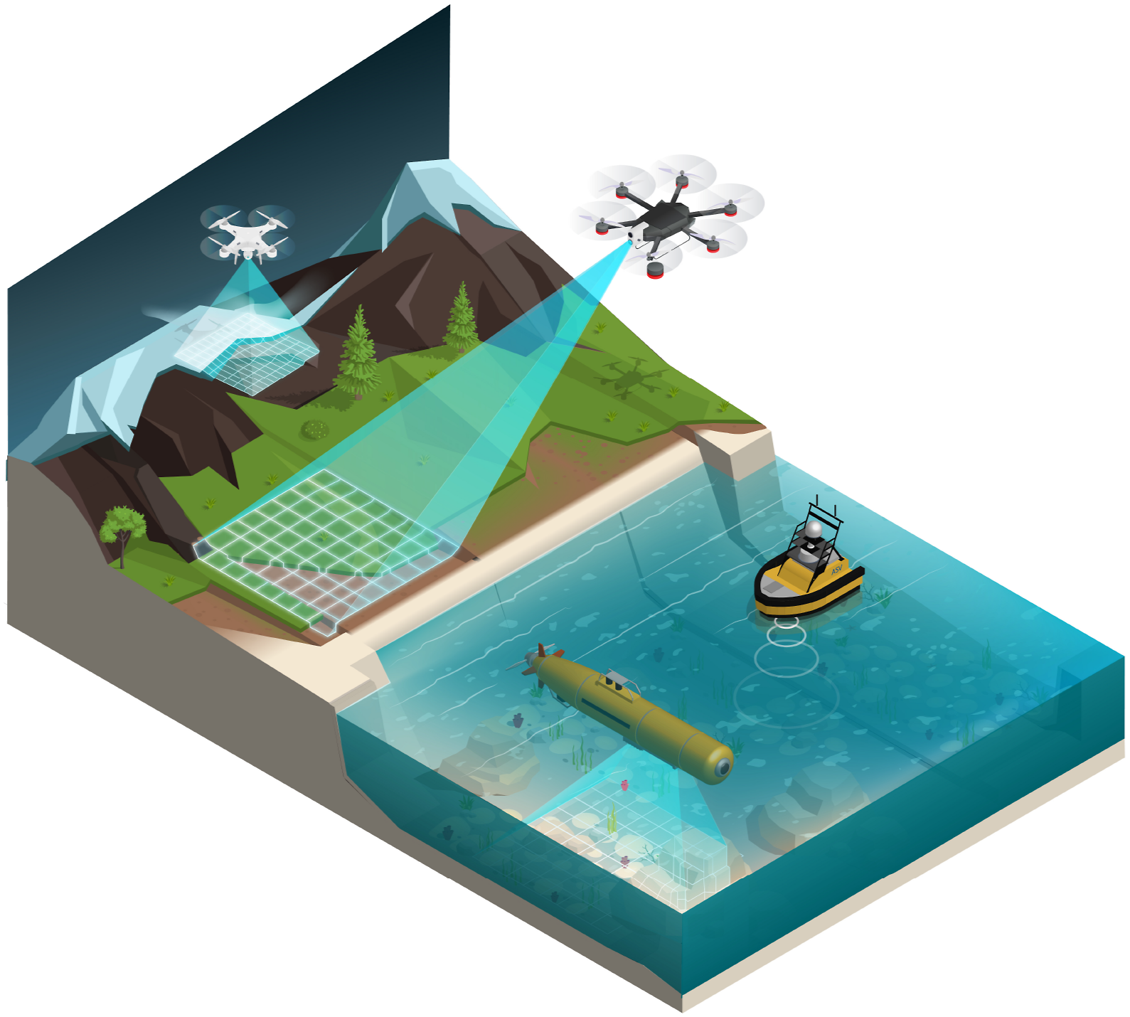
The SP problem seeks optimal fixed sensor locations to maximize the informativeness of collected data. Applications include determining sites for drilling ice cores to study glacial history or sampling soil to assess nutrient distribution (Krause et al., 2008; Shewry and Wynn, 1987; Wu and Zidek, 1992). In contrast, IPP focuses on planning optimal sensing paths for mobile robots, subject to constraints such as travel budgets and environmental boundaries. IPP applications range from autonomous surface vehicles monitoring ocean salinity to planetary rovers surveying the Martian surface (Hitz et al., 2017; Ma et al., 2018; Ott et al., 2024b). Similar challenges arise in active learning for machine learning (Ren et al., 2021) and next-best-view planning in robotics (Zeng et al., 2020), both of which can be viewed as broader generalizations of SP and IPP.
Learning paradigm Analogy: SP and IPP can be usefully framed by analogy to supervised, semi-supervised, and unsupervised learning in machine learning, though this analogy is not exact. The correspondence is conceptual: the “labels” in this analogy refer to measurements of the target phenomenon.
In the supervised analogy, densely distributed labeled data are assumed to be available prior to planning (Bigoni et al., 2020; Li et al., 2021; Semaan, 2017; Wang et al., 2020; Whitman et al., 2021). For example, optimal probe placement on printed circuit boards (PCBs) can be determined using detailed thermal images collected beforehand.
In the semi-supervised setting, only a sparse set of labeled data is available (Binney et al., 2013; Chekuri and Pal, 2005; Francis et al., 2019; Hitz et al., 2017; Krause et al., 2008; Singh et al., 2009). This is common in environmental monitoring, where a pilot mission may collect an initial sparse dataset (Kemna et al., 2018), which then guides subsequent, more informative data collection.
In the unsupervised analogy, no prior labeled data are available, and the robot must adaptively explore the environment. In IPP literature, this is often referred to as adaptive IPP (Bottarelli et al., 2019; Ma et al., 2018; Manjanna and Dudek, 2017; Mishra et al., 2018; Popović et al., 2024; Preston et al., 2024; Vivaldini et al., 2019), in which the mission usually iteratively alternates between planning and data collection. This contrasts with non-adaptive IPP, where the mission is fully planned before execution.
This article focuses on the semi-supervised SP and IPP problems and lays groundwork for future unsupervised extensions. Since both SP and IPP are NP-hard (Hollinger and Singh, 2009), practical solutions in real-world settings are typically approximate.
Closely related problems: Several related research areas are worth distinguishing.
Coverage problems, well-studied in robotics (Akbarzadeh et al., 2014; Bai et al., 2006; Bouman et al., 2022; Breitenmoser et al., 2010; Cortes et al., 2004; Ramsden, 2009; Sartoretti et al., 2022; Schwager et al., 2017), aim to sense every location in an environment given finite resources, with performance measured by coverage fraction. For example, Suryan and Tokekar (2020) addressed IPP for environmental monitoring using a disk-based coverage model. However, such methods do not explicitly exploit spatial correlations in the phenomenon, limiting their performance in non-stationary environments.
Another variant focuses on detecting hotspots—regions where the phenomenon of interest exhibits high activity (McCammon and Hollinger, 2021; Sung et al., 2021). In contrast, our objective is comprehensive monitoring for accurate data field reconstruction.
Information metrics: Semi-supervised SP and IPP are frequently addressed by maximizing information-theoretic measures such as mutual information (MI) or variance-based criteria (A-, B-, D-, and E-optimality). Each metric presents a distinct trade-off between computational cost and reconstruction accuracy; however, MI has been shown to consistently outperform both variance-based and Bayesian design criteria in terms of informativeness (Krause et al., 2008).
A common approach to addressing semi-supervised SP and IPP problems involves selecting sensing locations that maximize information-theoretic metrics. These metrics include, but are not limited to, mutual information (MI), variance, and various optimal experimental design criteria such as A-, B-, D-, and E-optimality. It is crucial to note that optimizing each metric yields different levels of environmental reconstruction accuracy, and more significantly, each carries a distinct computational cost.
Variance-based methods are computationally light but less informative. MI-based methods yield higher-quality sensing locations but require
Integer programming and convex optimization: A foundational approach to SP and IPP is to formulate them as integer programs or to solve them via convex optimization (Dutta et al., 2022; Joshi and Boyd, 2009; Ott et al., 2024b). This process typically begins by discretizing the environment and assigning an informativeness score to each candidate location, often using metrics such as variance or MI. The resulting problem is then expressed as either an integer program or a convex optimization problem.
However, reliance on discretization imposes notable limitations. It confines possible sensing locations to a finite subset of the environment and, more critically, causes computational cost to scale rapidly with discretization resolution. These drawbacks become particularly severe in complex 3D or spatio-temporal settings—especially when paired with computationally demanding metrics like MI—often rendering such approaches impractical for large-scale or real-time applications.
Discrete-space approaches: A classic line of work uses greedy algorithms to select high-variance points (Shewry and Wynn, 1987; Wu and Zidek, 1992). The recognition that MI is submodular (Binney et al., 2010; Krause et al., 2008; Krause and Guestrin, 2011) led to provably near-optimal greedy algorithms for SP and IPP. Extensions include stochastic greedy methods with variational GPs (Tajnafoi et al., 2021) and recursive greedy planners for IPP (Binney et al., 2013; Chekuri and Pal, 2005; Singh et al., 2009). These methods still require discretization, limiting spatial flexibility.
Continuous-space approaches: While greedy algorithms provide desirable approximation guarantees when maximizing submodular functions such as MI, non-greedy approaches in continuous domains often prioritize finding globally optimal sensor placements, sacrificing those guarantees in exchange for greater spatial flexibility. For example, Hollinger and Sukhatme (2014) developed IPP algorithms for continuous domains that maximize MI using rapidly-exploring random trees (RRTs), offering asymptotically optimal guarantees. Similarly, Asgharivaskasi et al. (2022) proposed a gradient-based method that employs a differentiable MI approximation, enabling continuous-space optimization.
A distinct family of continuous-space IPP methods employs ergodic control algorithms for settings where utility functions and ground truth field estimates are known (Miller et al., 2016; Rao et al., 2023). More general approaches, such as those by Hitz et al. (2017) and Popović et al. (2020), optimize sensing locations for arbitrary utility functions, often using genetic algorithms for maximization. Likewise, Francis et al. (2019) and Lin et al. (2019) applied Bayesian optimization to identify informative paths in continuous environments. However, derivative-free black-box optimizers—such as genetic algorithms and Bayesian optimization—tend to scale poorly with problem dimensionality, making them computationally inefficient for large or high-dimensional domains.
More recently, deep reinforcement learning (DRL) has been explored for IPP (Rückin et al., 2022). While promising, DRL requires substantial computational resources for generating diverse simulated datasets and training the policy. Furthermore, its ability to generalize to novel or unseen environments remains an open challenge.
Conclusion
We presented a fully differentiable formulation based on variational approximation to address the sensor placement (SP) problem and the informative path planning (IPP) problem. The formulation enabled the optimization of sensor placements in continuous domains using gradient-based approaches such as gradient descent and Newton’s method. We then showed that our formulation can be viewed as a special case of sparse Gaussian processes (SGPs) and leveraged their properties to present an upper bound on the asymptotic convergence rate of the formulation. Next, we generalized our approach to accommodate SP in discrete domains by leveraging the assignment problem to map continuous domain solutions to discrete domains efficiently. We then generalized the approach to handle sensors with non-point FoV shapes. Furthermore, we extended the approach to handle single and multi-robot informative path planning (IPP) while simultaneously accounting for differentiable path constraints and modeling continuous sensing robots.
Our experiments on real-world datasets demonstrated that our approach results in reconstruction quality being on par or better than the existing approaches while substantially reducing the computation time. We also demonstrated important capabilities of our approach, including an experiment showing SP for non-point FoV sensors in an environment with obstacles, SP and IPP with non-stationary kernel functions, distance-budget constrained IPP in a spatiotemporal environment, and IPP in a 3D environment with a non-point FoV sensor model that scales its FoV in proportion to the height from the ground similar to a camera. We also validated the IPP methods with field experiments using an autonomous surface vehicle deployed in a lake and an autonomous underwater vehicle deployed in the ocean to map the underwater surface.
This article lays a foundation for fully differentiable SP and IPP approaches that can find informative sensing locations while simultaneously accounting for any differentiable path constraints. Our recent work generalizes this approach to handle online adaptive IPP (Jakkala and Akella, 2025). Another interesting direction for future work is to incorporate the approaches into deep neural networks (DNNs) optimized for more complex downstream tasks or leverage pretrained DNNs in our approaches to accommodate high-level sensing location and path constraints that are difficult to formulate explicitly.
Footnotes
Acknowledgments
We are grateful to Artur Wolek and his students, Alex Nikonowicz, Michael Brancato, and Nicholas Kakavitsas, for providing access to their ASV platform and assisting us in setting up the ASV. We also thank Jacob Karty, Brian Faryadi, and Ninh Nguyen for their help with the ASV tests and experiments. We extend our thanks to Marios Xanthidis, Bert Tanner and his students, Vivek Mange and Chanaka Bandara, as well as Jason O’Kane and his students, Bennett Carley and Elias Sokolova, for their help with deploying the Aqua2 in Barbados. Finally, we thank Aidan Jackson, Ian Karp, Jeremy Mallette, and Nicholas Dudek from Independent Robotics for their assistance in setting up the Aqua2 ASV. This work was partly funded by the UNC Charlotte Office of Research and Economic Development and by NSF under Award Number IIP-1919233.
Author Contributions
Funding
The authors disclosed receipt of the following financial support for the research, authorship, and/or publication of this article: This work was funded in part by the UNC Charlotte Office of Research and Economic Development and by NSF under Award Number IIP-1919233.
Declaration of conflicting interests
The authors declared no potential conflicts of interest with respect to the research, authorship, and/or publication of this article.