
Abstract
Cable-driven compliant continuum robots (CCRs) can reach target areas in constrained spaces due to their elastic bodies being controlled remotely. They have been widely employed to inspect, maintain, or repair industrial machines such as gas turbine engines and oil pipes. However, their performances are usually limited by the low tip stiffness and the stiffness usually decreases with the increase of cable pulling forces. This paper aims to address the above problems by presenting a tip stiffness improved CCR formed by compliant anti-buckling universal joints (ACCR). The normalized nonlinear spatial models of the one-segment CCR and three-segment CCR are proposed and comprehensively verified using commercial nonlinear finite element analysis software. Given cable forces, prescribed cable displacements, tip loads, and gravity, the motion of any points on the CCRs can be analytically obtained. The performance characteristics of the one-segment CCRs and three-segment CCRs are extensively studied under different loading conditions, including the maximum CCR deformation, tip-location accuracy, shape dexterity, and tip stiffness. The results show that the tip stiffness of the ACCR is always much higher than that of the counterpart CCR under the same loading conditions. For example, the one-segment and three-segment ACCRs both have a high in-plane tip stiffness under in-plane actuation, which can increase by 49.0% and 31.3%, respectively; and they both have a high transverse tip stiffness under spatial actuation, which can increase by 48.9% and 31.2%, respectively. It is also confirmed that the ACCRs can increase tip stiffness by increasing cable actuation. Several preliminary planar experimental tests are carried out to validate the fabrication feasibility of the prototype, the accuracy of the analytical model, and/or the above-mentioned stiffness improvement.
1. Introduction
There has been a rapid increase in research on compliant continuum robots (CCRs) because they can bring potential advantages to many applications (S. Li and Hao, 2021). A CCR usually has a slender, elastic, and continuous shape, which is composed of multiple segments (Webster and Jones, 2010). It can enable access to confined spaces and ensures safe physical interactions with the surrounding environment, thanks to its exceptional flexibility. Dong et al. introduced a slender CCR for on-wing inspection or repair of gas turbine engines. Simaan and Taylor (2004) designed a CCR using multiple Nickel-titanium (NiTi) tubes with three distal dexterity units for laryngeal surgery. Amanov et al. (2021) designed an extensible CCR with path-following capabilities for minimally invasive surgery.
The performance of the majority of existing cable-driven CCRs is limited due to their low tip stiffness (Dong et al., 2022; Ji et al., 2020; Oliver-Butler et al., 2019; Ouabi et al., 2022; Smoljkic et al., 2014; Wang et al., 2018). The low tip stiffness of the CCRs driven by cables is mainly attributed to two coupled factors: the inherent small twisting stiffness (Dong et al., 2015) and negative load-dependent effects (associated with bending stiffness that decreases with the increase of cable forces) of constitutive joints/units. The following explanations show how low twisting stiffness in the structure reduces stiffness at the tip and how negative load-dependent effects contribute to low tip stiffness. The bending and twisting are depicted in Figure 1(f). Because the body’s centerline/backbone in deformation is not in line with that of the tip part, the twisting moment at the tip can bend partial non-proximal units of the CCR. Similarly, when a bending load acts at the tip of an actuated CCR, it can twist partial non-proximal units of the CCR. The smaller the twisting stiffness of the CCR, the lower the tip stiffness achieved. Most cable-driven CCRs are generally formed with modular compliant revolute/universal joints consisting of compressive flexures (Kutzer et al., 2011; Thomas et al., 2020; Wu et al., 2017; Zhang et al., 2021; Y. Zhao et al., 2024), where the cable forces only exert compression forces on these joints. The rotational/bending stiffness of these modular units usually decreases with the increase of cable forces, which is called the negative beam load-dependent effect (S. Li et al., 2022). Buckling may occur in CCRs if the cable force exceeds the critical load. Description of the ACCR: (a) modular unit Type 1, (b) modular unit Type 2, (c) exploded view of Type 1, (d) exploded view of Type 2, (e) a rotated inversion-based sheet under a compressive force, (f) a rotated non-inversion-based sheet under a compressive force, (g) simplified equivalent pseudo-rigid-body model for calculating the rotational stiffness of the deformed inversion-based sheet, (h) cable-loading positions, (i) spatial display of the ACCR, and (j) mimicking elephant’s trunk design-ACCR.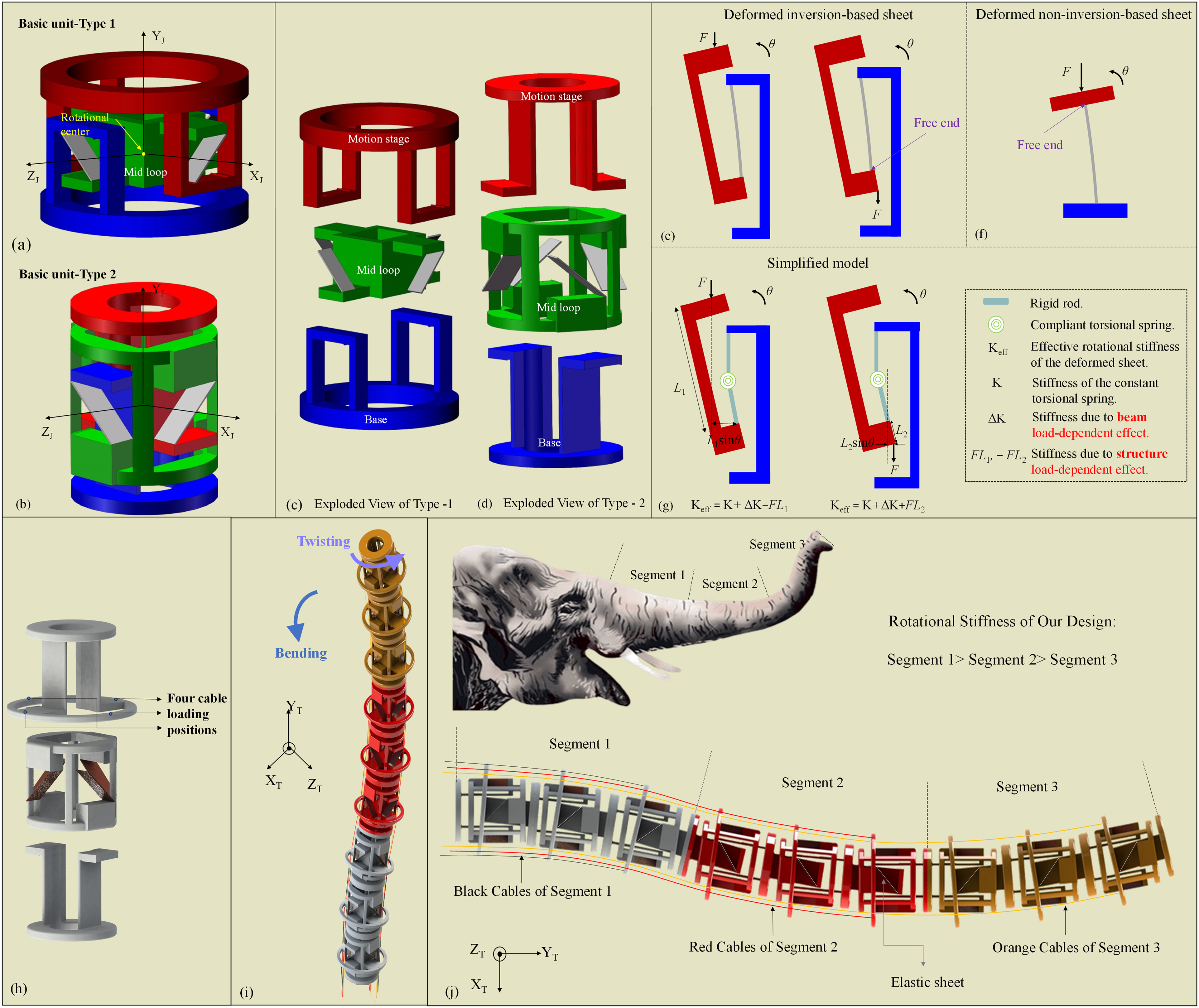
Many researchers are motivated to increase the stiffness of CCRs at different design levels. For example, at the bending segment design level, Langer et al. applied a reversible stiffening sheath for each bending segment by using dimension jamming (Clark and Rojas, 2019; Langer et al., 2018); Xing et al. employed low-melting-point alloy to obtain a solid phase for each segment (Xing et al., 2021). At the modular unit design level, Yang et al. added SMA alloys into each modular unit to lock robot movements (Yang et al., 2020); At the actuation level, Shiva et al. varied CCRs’ stiffness by antagonistically implementing two types of actuation (Hassan et al., 2017; Shiva et al., 2016; Stilli et al., 2017).
This paper focuses on improving the tip stiffness of cable-driven CCRs, whose elastic bodies can be controlled remotely. This improvement is achieved by incorporating anti-buckling universal joints (S. Li and Hao, 2021). CCRs using universal joints are quite common to have a much smoother curvature (in comparison with the revolute joints based CCR designs (Dong et al., 2015) with improved twisting stiffenss (compared with the wire-beam-backbone-based CCR designs (K. Xu et al., 2015). Many researchers designed CCRs using rigid universal joints combined with springs and multi-tendons (Hannan and Walker, 2000, 2001; Y. Liu et al., 2019b; Rone et al., 2018; Tang et al., 2017; Anderson, 1970; K. Xu et al., 2014; W. Xu et al., 2017; Yeshmukhametov et al., 2018; Yigit and Boyraz, 2017). In particular, K. Xu et al. developed a design specifically tailored for minimally invasive surgery (K. Xu et al., 2014). By incorporating rigid universal joints, they achieved a significant increase in twisting stiffness. Their work encourages us to design a CCR with compliant universal joints. To the best of our knowledge, no studies have reported the development of a CCR using a compliant universal joint with crossing spring pivots, which allows for a larger range of motion compared to existing compliant universal joints consisting of short sheets (Palmieri et al., 2012). The special advantage of the compliant universal joints is the intrinsic high rotational compliance in the degrees of freedom (DoF) direction and significantly high stiffness in the DoC (degrees of constraint) directions (S. Li and Hao, 2022). By introducing an inverse arrangement of the compliant universal joint, we can obtain an anti-buckling compliant universal joint, where its rotational (i.e., bending) stiffness can increase or remain constant by increasing cable forces (S. Li et al., 2022b). The compliant continuum robot utilizing anti-buckling compliant universal joints (ACCR) benefits from the distinct advantages of these joints. In other words, the tip stiffness of the ACCR can increase by increasing cable forces.
In the modeling method of the ACCR, we introduce a nonlinear spatial method utilizing the free-body diagram to derive a more accurate analytical model. There are many existing modeling methods for modeling the CCR, but they have some limitations as briefly listed as follows. (1) The center shifts of each anti-buckling universal joint should not be ignored, so the kinematic methods are not applied, such as DH method (Dong et al., 2015), constant curvature assumption (Goldman et al., 2014; Z. Li and Du, 2013; Nuelle et al., 2020; Webster and Jones, 2010), pseudo-rigid-body model (Venkiteswaran et al., 2019), and Bézier curve fitting (Yuan et al., 2017). In addition, these methods cannot effectively capture the nonlinearity of the ACCR; (2) The ACCR is not only limited to a very small ratio of cross-sectional dimension to its length, so its whole body cannot be simplified as a slender elastic rod. Therefore, Cosserat rod theory (Alqumsan et al., 2019; Caleb Rucker and Webster, 2014; Chikhaoui et al., 2019; Till et al., 2019, 2020; Till and Rucker, 2017) is not sufficient for capturing shear and twisting deformations of the ACCR. The thorough comparison between the proposed analytical model and existing analytical models for CCRs is summarized in Section 6.5.
While the anti-buckling universal joint itself is novel, its true significance lies in how it enables the construction of a new type of CCR. Specifically, the advantage of stiffness increase — a known bottleneck in most state-of-the-art CCRs— is discovered, analyzed, and validated through both finite element analysis (FEA) and experimental results in our work. We hope this can provide key insights to the community and enable a new generation of CCRs. The benefits and advantages of this CCR, made possible by the novel joint, extend far beyond the behavior of the joint itself, representing a broader scientific contribution. (1) Two types of CCRs have been proposed: the ACCR and its counterpart CCR (as a benchmark design), both utilizing universal joints with crossing spring pivots. Each type is represented by one segment featuring three universal joints or by three segments totaling nine universal joints. The CCR that uses anti-buckling universal joints with inversion-based sheets (ACCR) has a much higher stiffness compared to the CCR that uses universal joints with non-inversion-based sheets (the counterpart CCR). (2) The nonlinear spatial forward kinetostatic model of a CCR has been first derived, the system modeling framework in which can be used to model other CCRs with different compliant joints. Given any actuation and external loads (including cable forces, prescribed cable displacements, tip loads, and gravity), spatial displacements and rotations of any points on the stiffness improved CCR can be analytically obtained. (3) The performance characteristics including the tip stiffness of the ACCR and the counterpart CCR are thoroughly analyzed and compared under different geometric parameters and loading conditions, using both analytical and FEA models. (4) One-segment and three-segment prototypes are manufactured and experimentally tested. The modeling results have been rigorously verified through the utilization of nonlinear FEA and experiments. It has been experimentally confirmed that the tip stiffness of the one-segment ACCR can increase by increasing cable forces, and it is much larger than that of the one-segment counterpart CCR.
This paper is organized as follows. Section 2 describes the design of the CCR incorporating a series of anti-buckling universal joints. In Section 3, the normalized nonlinear spatial models of one-segment and three-segment CCRs are derived. The maximum CCR deformation, tip-location accuracy, shape dexterity, and tip stiffness improvement of the one-segment and three-segment CCRs are studied and verified with FEA and experiments in Sections 4 and 5, respectively. Section 6 discusses the effects of gravity, unaccounted considerations, scalability, reliability, and compares the three-segment ACCR with existing representative work. Conclusions and future work are finally drawn in Section 7.
2. Design description of the ACCR
We have presented two types of anti-buckling universal joints for the ACCR, as shown in Figure 1(a) and (b). Figure 1(c) and (d) are their exploded views, respectively. Each type of modular unit consists of four parts: a rigid base, a rigid middle loop, four elastic tensile sheets, and a rigid motion stage. The three rigid parts are not directly connected. The motion stage (red) and middle loop (green) are connected by a crossing spring pivot. The middle loop (green) and the base (blue) are connected by the other crossing spring pivot. Therefore, the three rigid parts are connected in series, which forms the anti-buckling universal joint. The only difference between the two types of modular units is the position of the middle loop. Type 1 has an internal middle loop, and Type 2 has an external middle loop. Type 1 and Type 2 joints have the same analytical model and experimental results in principle. More details on the design of these joints can be found in (S. Li et al., 2020b) and (S. Li and Hao, 2022).
Our design leverages the load-dependent effect of the compliant mechanism to increase ACCR stiffness by increasing cable actuation. This method provides an intrinsic way to enhance the ACCR’s stiffness. We use an elastic sheet as an example to demonstrate how load-dependent effects influence the stiffness of compliant mechanisms under applied loads. The load-dependent effects are classified in two types: structure load-dependent effects and beam load-dependent effects (S. Li et al., 2022). The structure load-dependent effect refers to how different loading positions can influence the stiffness of compliant mechanisms. The effective rotational stiffness of the deformed elastic sheet, denoted by Keff, is quite different when the loading position of the compressive force is near to or far from its free end, as shown in Figure 1(e) and (g). Small angle assumption (i.e., sinθ ≈ θ) is used for calculating the rotational stiffness associated with the structure load-dependent effect. The beam load-dependent effect refers to how a compressive or tensile axial force influences the stiffness of compliant mechanisms. The rotational stiffness of the deformed elastic sheet increases with the increase of tensile axial forces and decreases with the increase of compressive axial forces. We denote this variation in rotational stiffness caused by beam load-dependent effects as ΔK, where ΔK >0 when the elastic sheet is under a tensile axial force, otherwise ΔK <0. By comparing Figure 1(e) and (f), we can observe that a compressive force in the non-inversion-based sheet is converted into a tensile force in the inversion-based sheet. Therefore, by an inversion-based arrangement of elastic sheets, compressive forces exerted on the motion stage of the anti-buckling universal joint lead to tensile axial forces exerted on elastic sheets. The anti-buckling universal joints have the following features. (1) The four elastic sheets thereof are long compared to the ones with short sheets in (S. Li et al., 2020b), which leads to a large deformation universal joint rather than some existing compliant universal joints with a smaller range of motion (Dong et al., 2014; Palmieri et al., 2012). (2) Its rotational stiffness is customizable (i.e., the stiffness can be increased or kept constant) with the increase of cable forces by regulating its geometric parameters and loading positions, as verified in (S. Li et al., 2022; S. Li and Hao, 2022). (3) Its stiffness along any of the constraint/bearing directions (axial motion along the YJ-axis and twisting/rotational motion about the YJ-axis) is as high as desired, as detailed in (S. Li and Hao, 2022).
A hybrid active and passive cable-driven method is employed for actuating each segment, which implies that each segment is driven by four cables. Compared with the active cable-driven method (i.e., each universal joint is driven by four cables), the hybrid active and passive cable-driven method enables a lighter mechanism with fewer motors and reduced complexity for the control (T. Liu et al., 2018). The cable-loading positions of an anti-buckling universal joint are shown in Figure 1(h). ACCR should consist of at least two segments to obtain an “S” shape under a hybrid active and passive actuation. The assembly of three segments is considered to form the ACCR, as shown in Figure 1(i). The cables of segment 3 pass through all the motion stages of the universal joints in segments 2 and 1, and the cables of segment 2 pass through all the motion stages in segment 1 (Z. Li et al., 2017; T. Liu et al., 2019a; W. Xu et al., 2018), as shown in Figure 1(j). As each segment of the three-segment ACCR is driven by four cables, each segment obtains two degrees of freedom (DoFs), and the three-segment ACCR produces six DoFs in total.
From a bio-inspired perspective, the ACCR is designed with a gradually decreasing rotational stiffness along segments toward the tip, mimicking the biomechanical properties of an elephant’s trunk. In nature, this progressive stiffness variation allows an elephant’s trunk to maintain both strength at the base for load-bearing and flexibility at the tip for precise manipulation. Similarly, in our design as presented in Figure 1(j), the sheet width (or thickness) of the gray anti-buckling universal joint (proximal) is larger than that of the red one (middle), and the sheet width (or thickness) of the red one is larger than that of the orange one (distal). This stiffness variation allows the ACCR to achieve smooth and continuous deformations. Each segment consists of three anti-buckling universal joints with identical stiffness, ensuring uniform mechanical properties within each segment while maintaining the overall stiffness gradient across the segments. Additionally, segment 2 is rotated by −π/2 about the ACCR central axis (YT) in its undeformed state, in order to increase twisting stiffness about the YT-axis. The ACCR’s stiffness is increased by increasing cable actuation, aligning with the adaptive mechanics of an elephant’s trunk, as elephants can actively increase stiffness through muscle contraction.
3. Normalized nonlinear spatial models
Throughout this paper, we use the right-handed coordinate system and right-handed rule; use capital symbols to denote dimensional parameters, and use lower-case symbols to denote normalized (dimensionless) ones if not specified otherwise. All the load-equilibrium conditions are derived in a deformed condition, which means all the translational matrices and cable-force components are derived in a deformed condition. All the subscripts for nomenclatures of the normalized coordinates, translational matrices, and loads include their relative coordinate systems, for instance,
3.1. Kinetostatic model of a one-segment ACCR
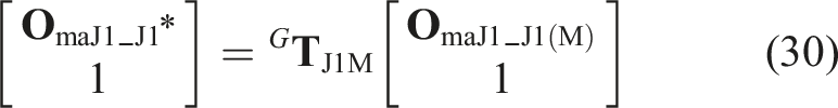
In this paper, the modeling procedure remains consistent regardless of the type of modular unit, with Type 1 serving as an illustrative example. As depicted in Figure 2(a), the one-segment CCR is composed of three anti-buckling universal joints (i.e., six inversion-based symmetric cross spring pivots (IS-CSP)) mounted in a serial arrangement. It is actuated with four cables. OG-XGYGZG denotes the global fixed coordinate system of the one-segment ACCR, which is located at the rotational center of the non-deformed anti-buckling universal joint 1, that is, OJ1. Two types of local mobile coordinate systems of the anti-buckling universal joint are denoted by OJΩ-XJΩYJΩZJΩ and OJΩ(M)-XJΩ(M)YJΩ(M)ZJΩ(M) (Ω = 1, 2, or 3). In the OJΩ-XJΩYJΩZJΩ system definition, OJ1-XJ1YJ1ZJ1 and OG-XGYGZG always overlap as shown in Figure 2(b), and the other two always accompany with the motion of the prior adjacent joint. In other words, OJ2-XJ2YJ2ZJ2 is located at OJ2 after the motions of the anti-buckling universal joint 1, and OJ3-XJ3YJ3ZJ3 is located at OJ3 after the motions of the anti-buckling universal joints 1 and 2. OJΩ(M)-XJΩ(M)YJΩ(M)ZJΩ(M) denotes the new local mobile coordinate system with regard to the corresponding OJΩ-XJΩYJΩZJΩ after rotations and translations of the universal joint-Ω (subscript (M) denotes mobile). The relationship between the OJΩ-XJΩYJΩZJΩ (Ω = 1, 2, or 3) and OJΩ(M)-XJΩ(M)YJΩ(M)ZJΩ(M) is formulated in Appendix A. Description of the one-segment ACCR: (a) cable-loading positions and the two overlapping coordinate systems: the global coordinate system OG-XGYGZG and local coordinate system OJ1-XJ1YJ1ZJ1, (b) two types of local coordinate systems of the three anti-buckling universal joints: OJΩ-XJΩYJΩZJΩ and OJ(M)Ω-XJ(M)ΩYJ(M)ΩZJ(M)Ω (Ω = 1, 2, or 3), respectively, and (c) the derivation of the cable-force components due to the cable force fc1.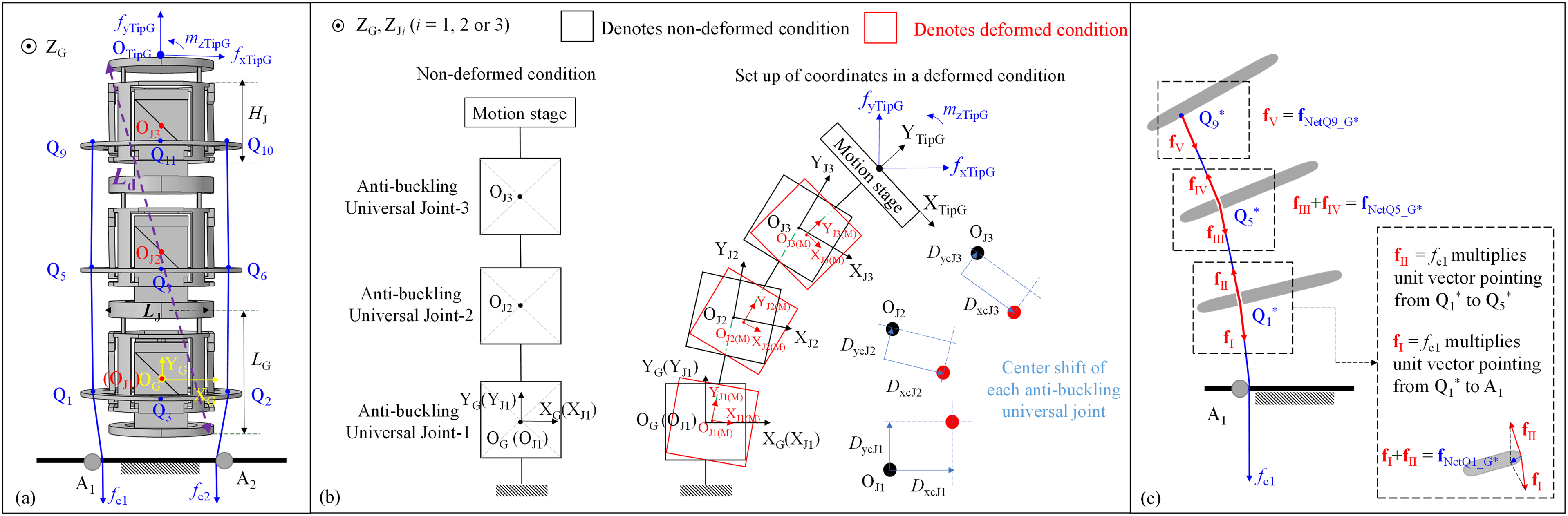
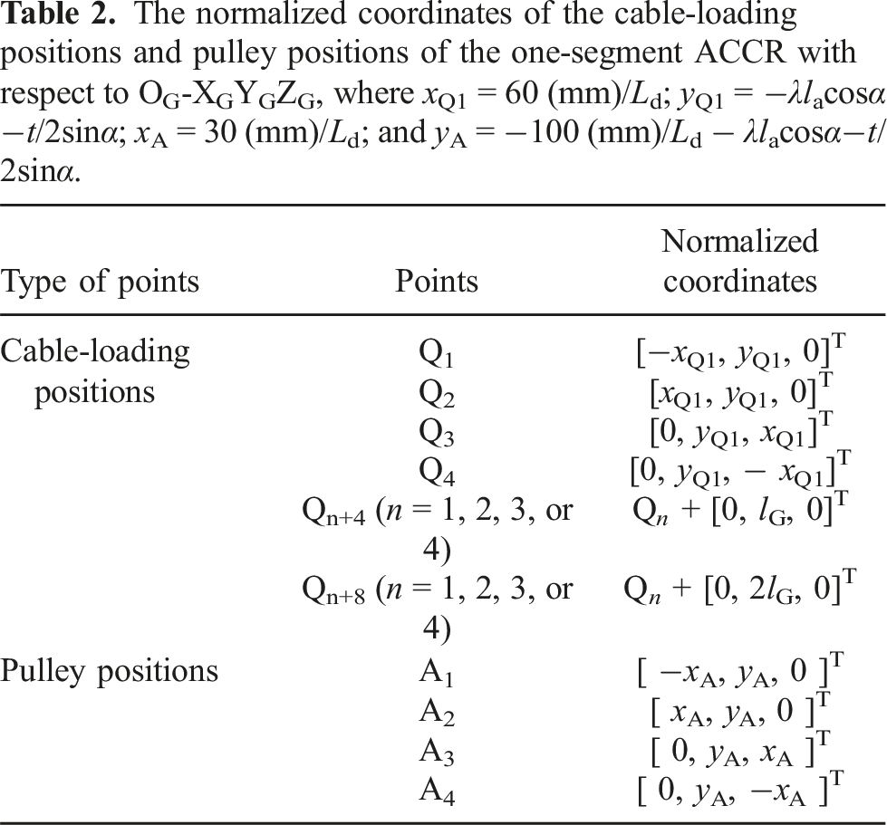
We use fxTipG, fyTipG, fzTipG, mxTipG, myTipG, and mzTipG to denote the tip loads with respect to OG-XGYGZG loading at tip OTipG. The directions for external forces or moments are based on the global fixed coordinate system throughout the motions of the one-segment CCR, as seen in Figure 2(a) and (b) for the tip loads. We use fcn (n = 1, 2, 3, or 4) to denote the normalized cable forces of cable-n, which is a positive constant along the cable-n; use A n (n = 1, 2, 3, or 4) and Q ε (ε = 1, 2, …, or 12) to denote the pulley positions and cable-loading positions of the one-segment ACCR, respectively, where A3 is in the front of A4, and two corresponding cables are not indicated in Figure 2(a). The four cables are fixed at Q9 to Q12 and pass through Q1 to Q8.
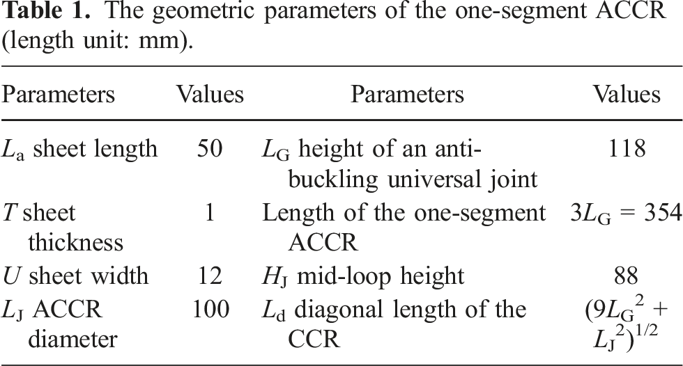
Ld denotes the characteristic length for normalization, which is equal to the diagonal length of the ACCR (cf. Figure 2(a)). All translational displacements and length parameters are divided by the footprint Ld. la, u, and t denote the normalized length, width, and thickness of each sheet, respectively. α, λ, h, lJ, and lG denote sheet tilt angle, crossing position, normalized loading position, the normalized diameter, and normalized height of the anti-buckling universal joint, respectively. They are the geometric parameters of the one-segment ACCR. Forces and moments are divided by EIz/Ld2 and EIz/Ld, respectively, where Iz denotes the cross-section moment and is expressed as UT3/12; E is Young’s modulus of the material. (For more details on the geometric parameters, the third figure in (S. Li and Hao, 2022) can be visited).
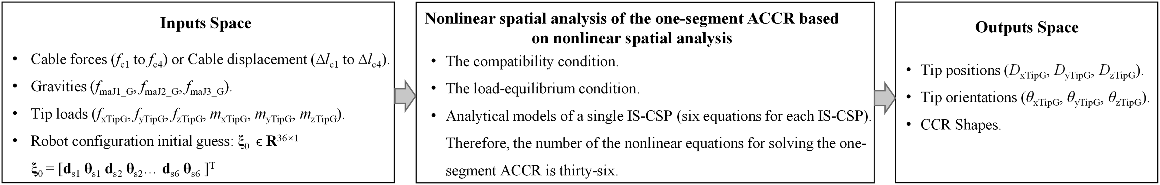
According to our previous work of modeling the IS-CSP (S. Li and Hao, 2022), given loading inputs (tip loads and cable forces) acting at the motion stage of the IS-CSP, translational displacements and rotations of the IS-CSP can be solved (six unknowns). We take each IS-CSP as a modular unit to model a one-segment ACCR, composed of six IS-CSPs, which makes a total of thirty-six unknowns. When geometric parameters (la, u, t, α, λ, h, lJ, and lG) and loading inputs of the one-segment ACCR with respect to OG-XGYGZG are given, the performances of the one-segment ACCR can be obtained by solving the load-equilibrium condition and compatibility condition (thirty-six equations in total) with an initial guess, which are summarized in Figure 3 and detailed below. Forward kinetostatic model of the one-segment ACCR.
We use


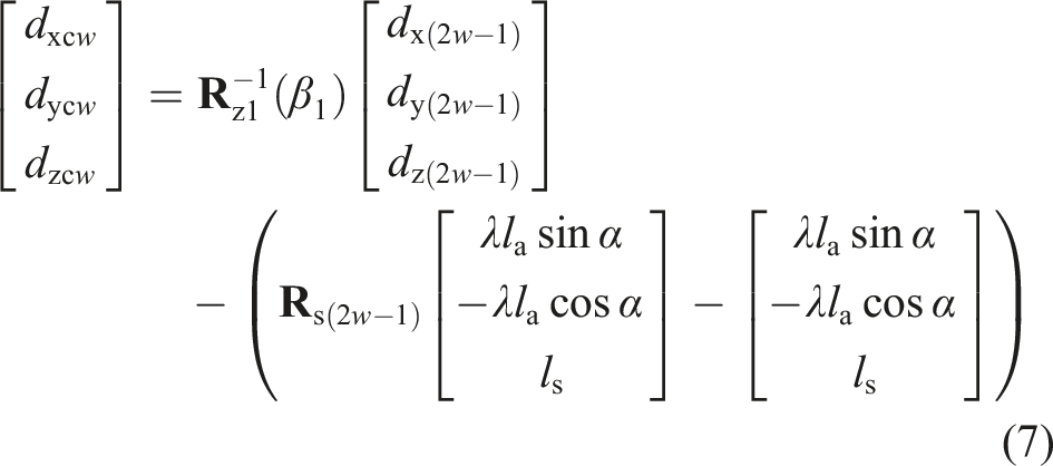
The normalized center shift of the anti-buckling universal joint-Ω (Ω = 1, 2, or 3) with respect to OJΩ-XJΩYJΩZJΩ is denoted by
All cable-force components due to fc1 through fc4 acting on the cable-loading positions in a deformed condition with respect to OG-XGYGZG should be obtained first. They are denoted by
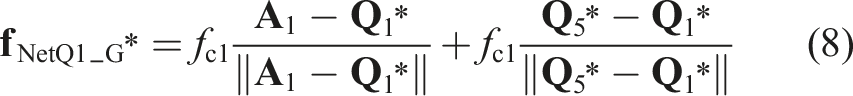
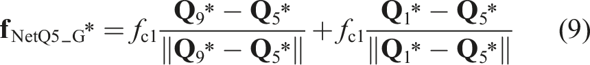
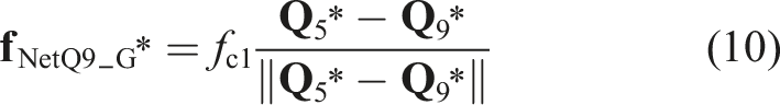
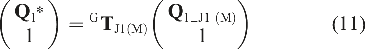
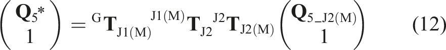
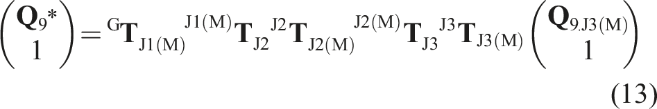
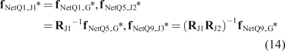
Therefore, the cable-force components loading at Q1*, Q5*,, and Q9* with respect to OJ1-XJ1YJ1ZJ1, OJ2-XJ2YJ2ZJ2, and OJ3-XJ3YJ3ZJ3, respectively, are formulated in equation (14). Other cable-force components due to fc2 through fSc4 can be derived similarly.
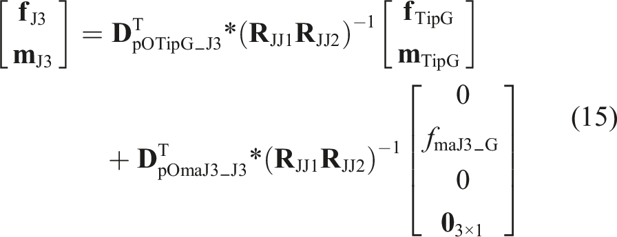
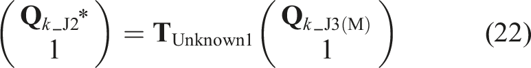
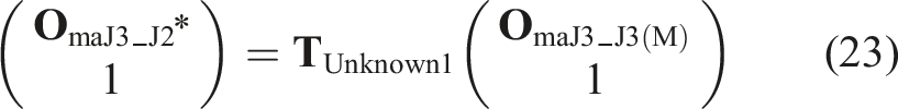
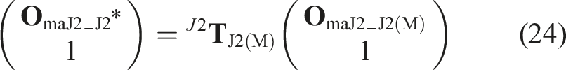
Then all the loading inputs, including tip loads and cable-force components with respect to OG-XGYGZG, should be equivalently converted to the loads with respect to OJΩ-XJΩYJΩZJΩ (Ω = 1, 2, or 3) for each anti-buckling universal joint in a deformed condition. The cable-force components loading at Q1*–Q4* have been considered in the analytical modeling of the anti-buckling universal joint 1, similarly to the cable-force components loading at Q5*–Q8*, and Q9*–Q12* have been considered in the analytical modeling of an anti-buckling universal joints 2 and 3. The load-equilibrium condition for each single IS-CSP is completed. The load-equilibrium condition between different universal joints should be further derived because the loads loading at the top joint influence the motions of its underneath joints. For instance, the cable-force components loading at the anti-buckling universal joint 3 and tip loads with respect to OG-XGYGZG, lead to moments acting at the anti-buckling universal joint 2. We use fxJΩ, fyJΩ, fzJΩ, mxJΩ, myJΩ, and mzJΩ, to denote normalized loads of the anti-buckling universal joint-Ω acting at OJΩ with respect to OJΩ-XJΩYJΩZJΩ, respectively. The load-equilibrium condition of the one-segment ACCR is formulated as equations (15), (20), and (25).
We assume each anti-buckling universal joint has the gravity located at its rotational center. Equation (15) shows the load-equilibrium condition of the anti-buckling universal joint 3 with respect to OJ3-XJ3YJ3ZJ3, which is formulated due to the tip loads and the gravity of the anti-buckling universal joint 3.
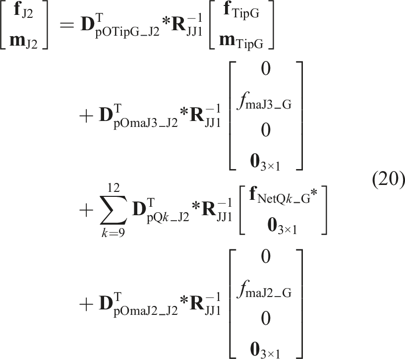
Equation (20) shows the load-equilibrium condition of the anti-buckling universal joint 2 with respect to OJ2-XJ2YJ2ZJ2 due to the effects of tip loads, gravity, and cable-force components loading at anti-buckling universal joint 3, and gravity of the anti-buckling universal joint 2.
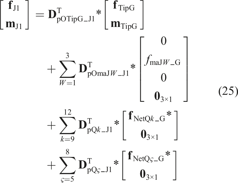
Equation (25) formulates the load equilibrium of the anti-buckling universal joint 1 with respect to OJ1-XJ1YJ1ZJ1 due to the effects of tip loads, gravity, cable-force components loading at anti-buckling universal joint 3; gravity and cable-force components loading at anti-buckling universal joint 2; and gravity of the anti-buckling universal joint 1.
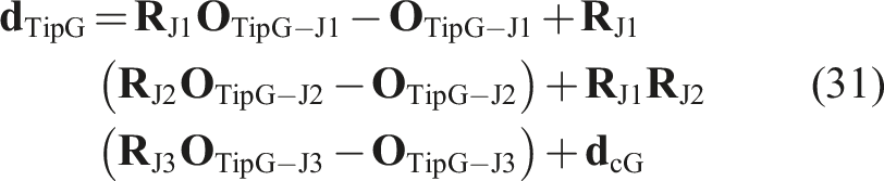
The normalized tip displacements are denoted by


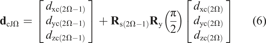
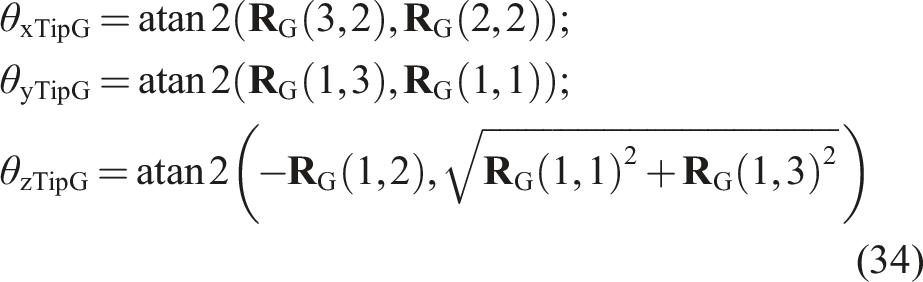
As we determine the rotational sequence of all the rotational matrices in equation (1), the three rotations at the tip OTipG (denoted by θxTipG, θyTipG, and θzTipG) are derived as (34).
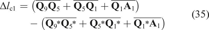
The cable displacement is the result of the cable length in a non-deformed condition minus the cable length in a deformed condition. The normalized cable displacements of the four cables are then found as equation (35) through (38). When ∆lcn > 0, the cable is pulled down, otherwise, the cable is elongated.
3.2. Kinetostatic model of a three-segment ACCR
Figure 4(a) depicts the front view of the three-segment ACCR, including the cable-loading positions and coordinate systems. Each segment has three anti-buckling universal joints and is actuated by four cables. The cables of segment 3 go through the motion stages of segments 2 and 1. The cables of segment 2 go through the motion stages of segment 1. We use OT-XTYTZT to denote the global coordinate system of the three-segment ACCR; use OGΩ-XGΩYGΩZGΩ (Ω = 1, 2, or 3) to denote the local coordinate systems of segment Ω in Figure 4(b); use fSE1-cn, fSE2-cn, and fSE3-cn (n = 1, 2, 3, or 4) to denote the positive tensions along cable-n of segments 1, 2, and 3, respectively, as shown in Figure 4(c); use fxTip, fyTip, fzTip, mxTip, myTip, and mzTip to denote the tip loads with respect to OT-XTYTZT loading at tip OTip; use QwSE1, QwS2S1, and QwS3S1 (w = 1, 2, …,12) to denote the cable-loading positions acting at segment 1 due to the cables of segments 1, 2, and 3, respectively; use QwSE2 and QwS3S2 to denote the cable-loading positions acting at segment 2 due to cables of segments 2 and 3, respectively; use QwSE3 to denote the cable-loading positions acting at segment 3 due to cables of segment 3. Description of the three-segment ACCR: (a) section view from XY plane of the cable-force loading positions, (b) global coordinate system OT-XTYTZT and local coordinate systems OGΩ-XGΩYGΩZGΩ (Ω = 1, 2, or 3), and (c) top view of the cables in each segment.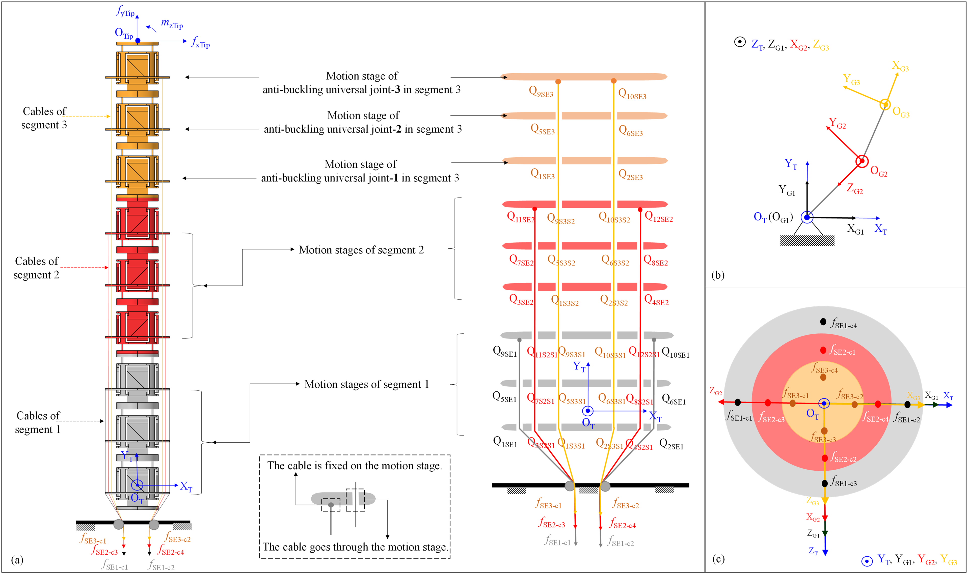
We take each anti-buckling universal joint as a modular unit to model a three-segment ACCR. Given geometric parameters, tip loads, and cable forces of the three-segment ACCR, all loading inputs with respect to OT-XTYTZT should be equivalently converted to the loads with respect to OJΩ-XJΩYJΩZJΩ (Ω = 1, 2, or 3) for each anti-buckling universal joint. The displacements and rotations of the nine anti-buckling universal joints can be obtained by solving the nonlinear spatial models of the anti-buckling universal joints and load-equilibrium condition of a three-segment ACCR in a deformed condition. Then any points on the three-segment ACCR can be obtained by solving the compatibility condition in a deformed condition, such as tip-location and shape dexterity.
The normalized cable-force components with respect to OT-XTYTZT acting at each segment are derived firstly using the same method in Section 3.1. We use fxJΩSE1, fyJΩSE1, fzJΩSE1, mxJΩSE1, myJΩSE1, and mzJΩSE1 to denote normalized loads of the anti-buckling universal joint-Ω acting at its rotational center, OJΩSE1, with respect to OJΩSE1-XJΩSE1YJΩSE1ZJΩSE1 in segment 1, respectively (segments 2 and 3 have similar nomenclatures).
The load-equilibrium condition of the three-segment ACCR includes the load-equilibrium conditions between each anti-buckling universal joint. The load-equilibrium condition of the anti-buckling universal joints in segment 3 is the same as those of Section 3.1. However, more cable-force components and gravities should be considered for those of segments 1 and 2, in terms of two aspects: (1) The cable-force components acting at the motion stages due to other segments’ cables should be added for the modeling of anti-buckling universal joints. (2) Gravities and cable-force components acting at the top anti-buckling universal joints affect the motions of bottom anti-buckling universal joints, which should be added for the load-equilibrium condition between different anti-buckling universal joints.
We take the anti-buckling universal joint 3 in segment 2 as an example. In the modeling of this modular unit, the load-equilibrium condition should include cable-force components due to other segments’ cables, that is, the cable-force components loading at QkS3S2 (k = 9, 10, 11, or 12). Reference (S. Li and Hao, 2022) gives a generalized analytical model for the modeling of an anti-buckling universal joint.
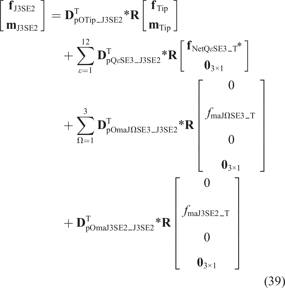
Equation (39) shows the load-equilibrium condition of the anti-buckling universal joint 3 in segment 2 with respect to its local coordinate system, OJ3SE2-XJ3SE2YJ3SE2ZJ3SE2, due to effects of loads that act at other anti-buckling universal joints and its gravity. In the right side of equation (39), the items, in turn, are formulated due to the effects of tip loads, cable-force components loading at the motion stages of the three anti-buckling universal joints in segment 3, gravities of the three anti-buckling universal joints in segment 3, and the gravity of the anti-buckling universal joint 3 in segment 2. Therefore, the load-equilibrium condition of other anti-buckling universal joints in segments 1 and 2 can be similarly derived.

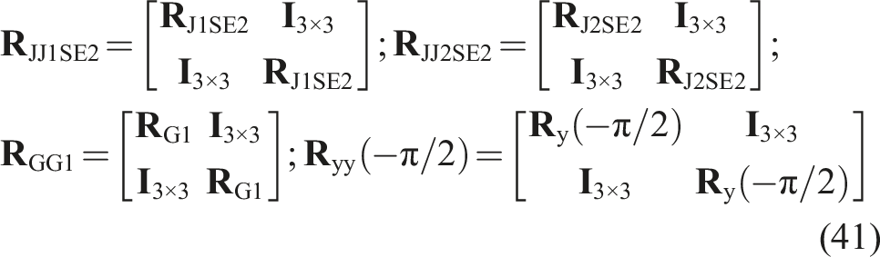
The rotational matrix for segment Ω with respect to OGΩ-XGΩYGΩZGΩ (Ω = 1, 2, or 3) is written in equation (42).

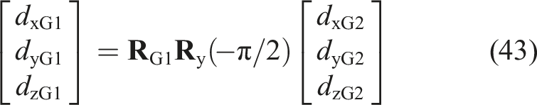
As segment 2 rotates by −π/2 about both segments 1 and 3, the normalized displacements of segment 2 with respect to OG2-XG2YG2ZG2 can be described by those with respect to OG1-XG1YG1ZG1, as shown in equation (43).
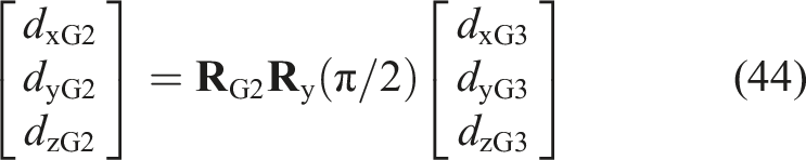
The normalized displacements of segment 3 with respect to OG3-XG3YG3ZG3 can be described by those with respect to OG2-XG2YG2ZG2, as shown in equation (44).
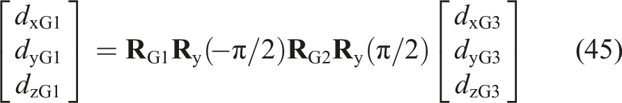
Combining equations (43) and (44), the normalized displacements of segment 3 with respect to OG3-XG3YG3ZG3 can be described by those with respect to OG1-XG1YG1ZG1, as shown in equation (45).
Therefore, the rotational compatibility condition of the three-segment ACCR is derived in equation (46).

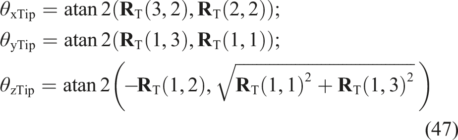
If we determine the rotational sequence is the same as equation (1), the three rotations of the three-segment ACCR (denoted by θxTip, θyTip, and θzTip) can be calculated as equation (47).
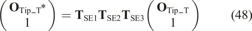
The normalized coordinate of a point on the ACCR in a deformed condition is derived depending on its position. Equation (48) gives the normalized coordinates of the tip OTip with respect to OG-XGYGZG in a deformed condition. The normalized coordinates of other points on the three-segment ACCR with respect to OG-XGYGZG in a deformed condition can be similarly derived.
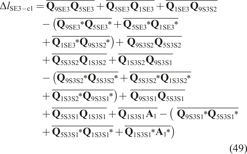
The cable displacements of the four cables for each segment can be derived in a similar way to what we did in Section 3.1. The normalized cable displacement of cable-1 in segment 3 is taken as an example, as shown in equation (49).
4. Spatial Analysis of the one-segment ACCR
In this section, the accuracy of the kinetostatic model of the one-segment ACCR is assessed by using the nonlinear FEA model, which is built in COMSOL 5.0. In the FEA model, the mesh size of the parts excluding elastic sheets is not required but they should be set as “rigid domain” in COMSOL 5.0. The scale factor of the total displacement figures given by the COMSOL 5.0 is set to 1, which means the deformation is not being enlarged or reduced. The details of the FEA process are shown in Appendix B.
The geometric parameters of the one-segment ACCR (length unit: mm).
The normalized coordinates of the cable-loading positions and pulley positions of the one-segment ACCR with respect to OG-XGYGZG, where xQ1 = 60 (mm)/Ld; yQ1 = −λlacosα −t/2sinα; xA = 30 (mm)/Ld; and yA = −100 (mm)/Ld − λlacosα−t/2sinα.
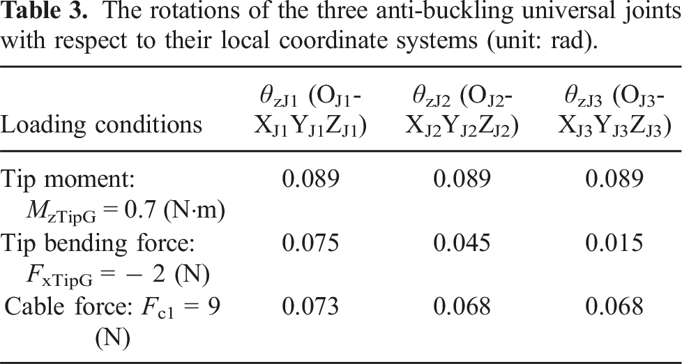
The rotations of the three anti-buckling universal joints with respect to their local coordinate systems (unit: rad).
4.1. Maximum ACCR deformation
Figure 5(a) and (b) show the tip motions of analytical and FEA results of the one-segment ACCR under tip moments and tip forces. Three tip forces remain constant (FxTipG = FzTipG = 5 (N), FyTipG = − 5 (N)) and two tip moments are equal to each other (MxTipG = MzTipG) ranging from 0 to 0.5 (N·m) with a step of 0.1 (N·m). The average errors between the analytical and FEA results of DxTipG, DyTipG, DzTipG, θxTipG, θyTipG, and θzTipG, are 6.4%, 7.3%, 4.5%, 5.2%, 7.4%, and 6.8%, respectively. The maximum deformation of the one-segment ACCR is shown in Figure 5(c) for MxTipG = MzTipG = 0.5 (N·m) and the maximum Von Mises stress is 7.65 ×10⁸ (Pa). Maximum deformation evaluation under two moments and three forces acting at the tip of the one-segment ACCR: (a) tip displacements, (b) tip rotations, and (c) total displacements under three constant tip forces and two equal moments.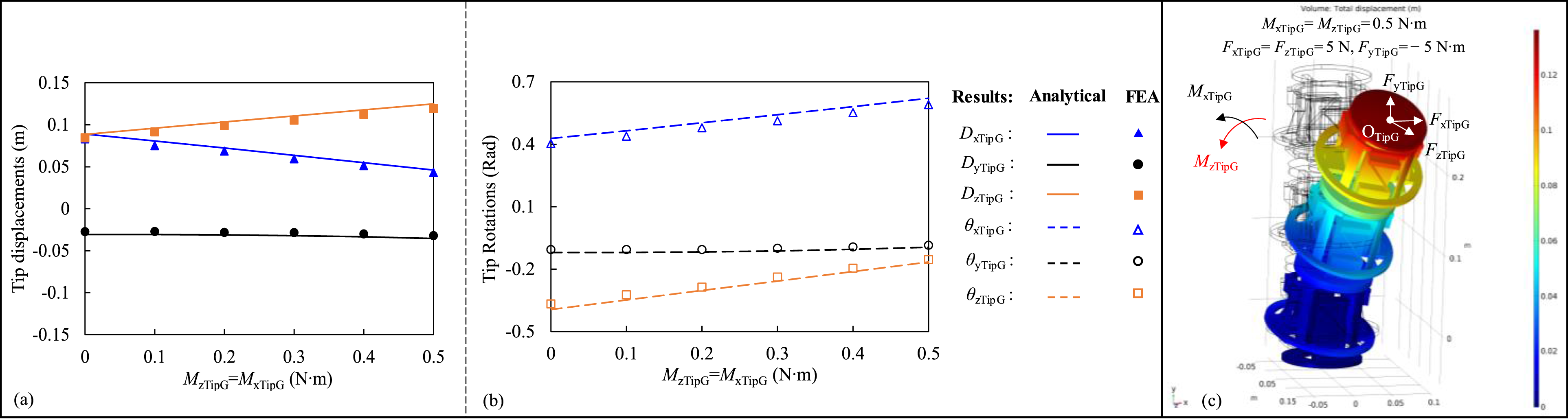
The corresponding tip displacements and rotations are DxTipG = 0.046 (m), DyTipG = − 0.035 (m), DzTipG = 0.125 (m), θxTipG = 0.621 (rad), θyTipG = − 0.095 (rad), and θzTipG = − 0.166 (rad), that is, 35.6°, 5.45°, and 9.52°, respectively. Note that throughout the paper, the rotational angles are the Euler angles, not the roll-pitch-yaw angles. Therefore, the tip rotations are not the ACCRs’ bending or twisting angles.
4.2. Tip-location accuracy and shape dexterity
The tip-location accuracy and shape dexterity of the one-segment ACCR are studied when α = 45° and the ACCR is driven by cable forces. The cable forces: Fc1 ranges from 1 (N) to 9 (N) with a step of 2 (N), Fc3 = 5 (N), and other cable forces are equal to 0. From the analytical model, all cable-force components in a deformed condition can be calculated, which are used to be point loads loading at the cable-loading positions Q1 to Q12 in the FEA model. Then the displacements of any point with respect to OG-XGYGZG in the FEA model can be evaluated by using “Point Evaluation” in COMSOL 5.0. Shape dexterity of the one-segment ACCR with respect to OG-XGYGZG: (a) tip displacements, (b) tip rotations, (c) shape dexterity with the increase of Fc1, (d) total displacement under Fc1 = 1 (N), (e) total displacement under Fc1 = 3 (N), and (f) total displacement under Fc1 = 9 (N). (Average differences between the analytical results and their corresponding FEA results in Figure 6(a) and (b): DxTipG: 5.8%, DyTipG: 8.5%, DzTipG: 5.2%, θxTipG: 5.6%, θyTipG: 7.8%, and θzTipG: 3.3%. The average differences of the coordinates between the analytical and FEA ACCR shapes in Figure 6(c) with respect to XG, YG, and ZG-axes are 2.9%, 2.3%, and 2.3%, respectively).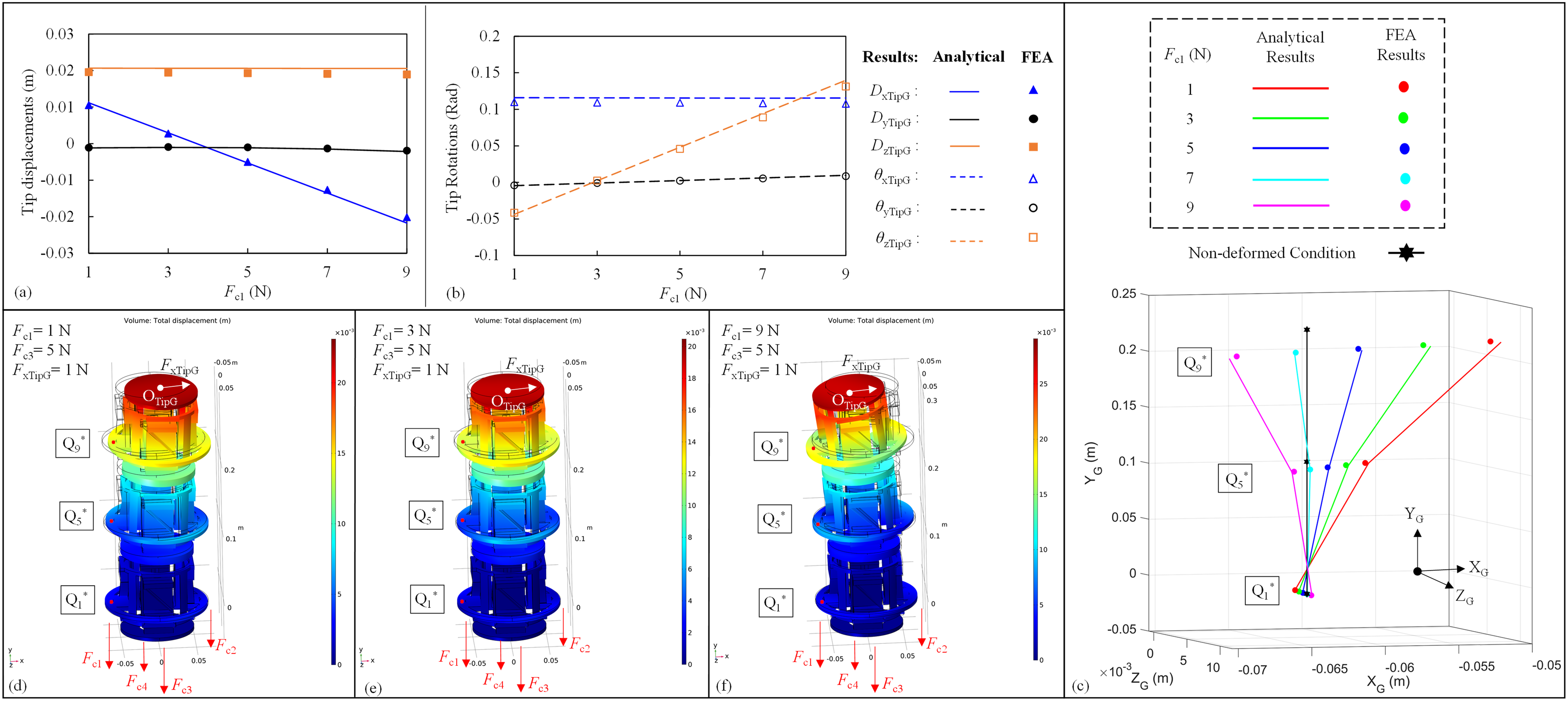
4.3. Tip-stiffness improvement
We first study the in-plane and the out-of-plane tip stiffness of the one-segment ACCR and counterpart CCR under two different in-plane actuations. Then the transverse tip stiffness of the two CCRs under a spatial actuation is investigated.
A counterpart CCR composed of non-inversion-based crossing spring pivots is built and plays as a comparative group. The counterpart CCR is representative of the stiffness characteristics of CCR designs reported in the literature. The tip stiffness of the counterpart CCR decreases with the increasing cable actuation. As we stated in the Introduction, the performance of many existing cable-driven CCRs is limited due to their low tip stiffness. The counterpart CCR is the most appropriate choice as a comparative design for the following reasons. The primary factors influencing the performance characteristics of different CCRs are the cable actuation, joints, and structural features. In both the ACCR and the counterpart CCR, the cable-loading positions are located at the free-end planes of each elastic sheet, with equal actuation forces applied. Both designs utilize the same compliant universal joints, with the only difference coming from the arrangement of joints in terms of an inversion-based configuration or non-inversion-based configuration. Thereby, we can reasonably compare the stiffness of the two designs while eliminating the influence of the CCR’s structural features on the results.
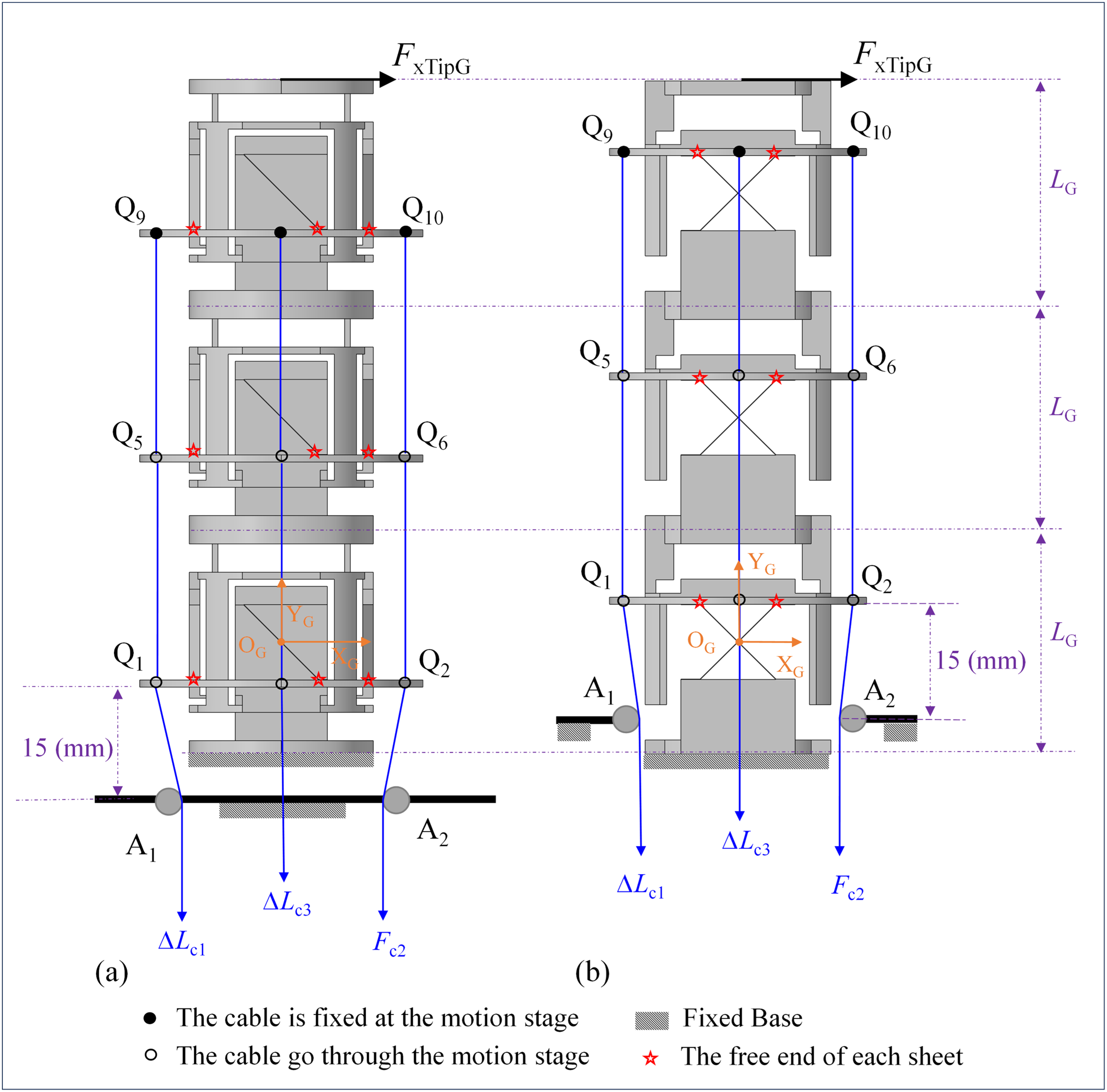
We require all the geometric parameters of ACCR and the counterpart CCR to be the same, and cable-force loading positions to be located at the level of the sheets’ free ends for each universal joint of the two CCRs, as shown in Figure 7. K∆Fx-∆Dx denotes the in-plane tip stiffness along the XG axis, which can calculated as equation (50) (Mahvash and Dupont, 2011; Yang et al., 2020). We use K∆Fz-∆Dz to denote the out-of-plane tip stiffness along the ZG axis, which can be computed similarly. Description of the two CCRs: (a) ACCR and (b) the counterpart CCR (α = 45° here and cable-4 is not drawn).
The improvement ratio of the in-plane tip stiffness is given as equation (51). The improvement ratio of the other stiffness can be solved similarly.
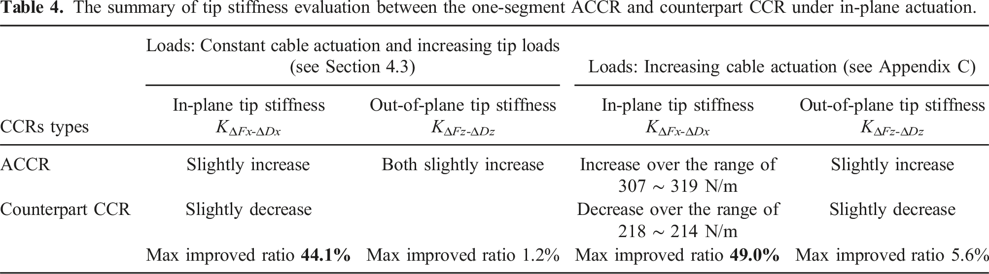
λ takes 0.5, α = 15°, 30°, or 45°, and the loading condition is an increasing tip force FxTipG with a constant cable-displacement actuation ∆Lc1. ∆Lc1 is fixed at 4 (mm) and other cables are free. These loading conditions are held in the following two situations. (i) To compare in-plane tip stiffness K∆Fx-∆Dx of the ACCR and counterpart CCR, the in-plane tip load FxTipG ranges from 0.2 (N) to 1.6 (N) with a step of 0.2 (N). Their results are compared in Figure 8(a). The maximum difference between the analytical and FEA results is 3.9%. K∆Fx-∆Dx_ACCR has high values for α = 15°. However, K∆Fx-∆Dx_coun has low values for the same α. K∆Fx-∆Dx_ACCR is larger than K∆Fx-∆Dx_coun, and K∆Fx-∆Dx_ACCR increases by 44.1%, 38.8%, and 30.1% under α = 15°, 30°, or 45°, respectively. (ii) To compare the out-of-plane tip stiffness K∆Fz-∆Dz of the ACCR and counterpart CCR, the out-of-plane tip load FzTipG ranges from 0.2 (N) to 1.6 (N) with a step of 0.2 (N). Their results are as shown in Figure 8(b). The maximum difference between the analytical and FEA results is 5.4%. K∆Fz-∆Dz of the two CCRs have high values for α = 15°. K∆Fz-∆Dz of the two CCRs are close but K∆Fz-∆Dz_ACCR is slightly higher than K∆Fz-∆Dz_coun, where K∆Fz-∆Dz_ACCR and K∆Fz-∆Dz_coun denote the out-of-plane tip stiffness of the ACCR and counterpart CCR, respectively. K∆Fz-∆Dz_ACCR increases by 1.2%, 0.9%, and 0.6% under α = 15°, 30°, or 45°, respectively. The in-plane and the out-of-plane tip stiffness comparison between the one-segment ACCR and counterpart CCR under a constant cable-displacement actuation and increasing tip forces: (a) the in-plane tip stiffness K∆Fx-∆Dx under a series of increasing FxTipG and (b) the out-of-plane tip stiffness K∆Fz-∆Dz under a series of increasing FzTipG.
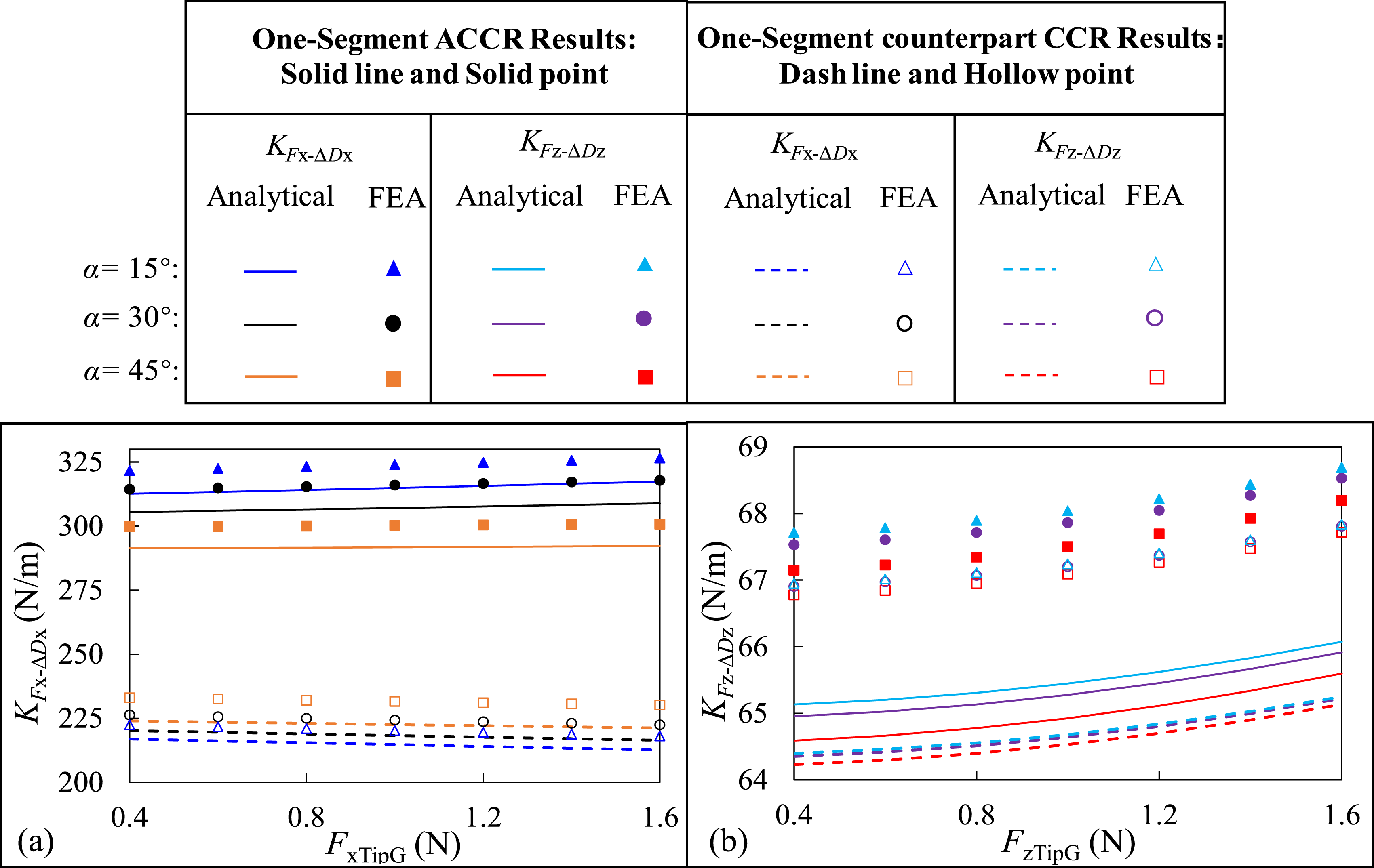
The summary of tip stiffness evaluation between the one-segment ACCR and counterpart CCR under in-plane actuation.
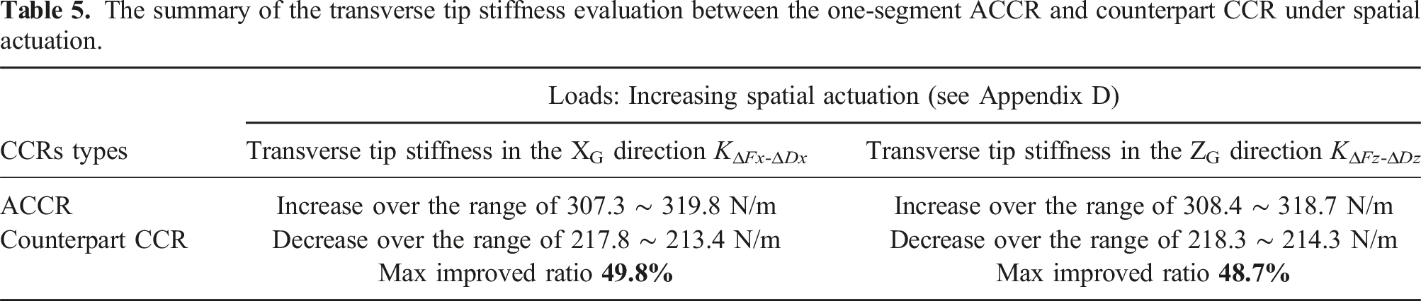
The summary of the transverse tip stiffness evaluation between the one-segment ACCR and counterpart CCR under spatial actuation.
4.4. Experiment
The deformation, shape dexterity and tip stiffness have been thoroughly analyzed in Sections 4.2 using analytical models and FEA. In this section, the experimental comparison between the ACCR and counterpart CCR is investigated. Each fabricated prototype is shown for verifying design and modeling but is not optimized for specified size and performance. We use Type 1 joints to construct the ACCR instead of Type 2 joints, primarily due to its ease of fabrication.
Appendix E details two fabrication methods for the proposed robot, resorting to 3D printed parts and their assembly. The use of a 3D printer can lead to a low-cost and lightweight prototype over a short lead period. Therefore, the material for elastic sheets and the design parameters of the CCR are different from those mentioned earlier in the analytical and FEA studies. All 3D printing material is selected to be PLA where its Young’s modulus is 3150 (MPa) and Poisson’s ratio is 0.35. The fill density was set to be 50%. These parts are connected with each other by using Grease Welding Flux, which is a high-strength glue for professional industrial applications. Each anti-buckling universal joint has a weight of close to 22 (g). The length of the tip marker is 14 (mm) and the mass of the tip marker is 1 (g). The cable is made of strong nylon with a transparent color, which has trivial elongation. We use different weights to apply cable forces and tip forces.
The prototypes of the two one-segment CCRs using fabrication method 1 of Appendix E are shown in Figure 9(a) and (b). The geometric parameters are shown in Table 6. We compare the in-plane tip stiffness due to the significant improvement observed in Section 4.3. We designed a limiter for the CCR, which means the rigid parts of the CCR will contact to avoid excessive loads, as shown in Figure 9(c). Therefore, the maximum cable force that can be applied to the one-segment CCR is 50 (g) and the corresponding maximum cable displacement calculated by the analytical model is 4 (mm). Fabrication parts for the two one-segment CCRs: (a) parts for fabrication of a counterpart universal joint, (b) parts for fabrication of an anti-buckling universal joint, and (c) prototypes of the two joints. Geometric parameters of the one-segment CCRs using fabrication method 1.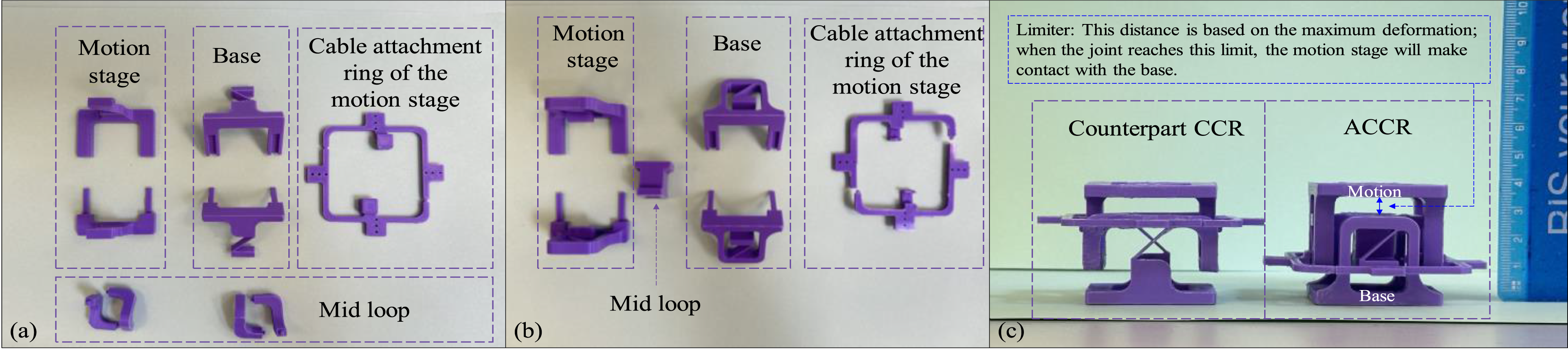
Two tests are carried out. Each prototype is fixed on the working bench, as depicted in Figure 10(a). Test 1 is designed to investigate the tip stiffness of the ACCR and counterpart CCR under conditions of an increasing tip force and a constant cable displacement, as shown in Figure 10(b). The tip load can be calculated using equation (52). Test 2 is designed to investigate the tip stiffness under conditions of an increasing cable force and a constant cable displacement, as shown in Figure 10(c). Test setup for the tip stiffness evaluation of the ACCR and the counterpart CCR: (a) prototype of the ACCR is unloaded, (b) prototype of the ACCR in Test 1, and (c) prototype of the counterpart CCR in Test 2.
We use 1/8-inch graph paper and an HD camera to calculate the tip motions of the CCR, as shown in Figure 11(a). The HD camera should face directly opposite the tip and photograph a series of figures when the loads change. The tip displacements can be calculated by counting the number of squares in the graph paper. In Test 1, the mass for providing tip force ranges from 0 (g) to 50 (g) with a step of 10 (g), and the cable displacement ΔLc1 is constant at 4 (mm), so that the stiffness results for the ACCR and the counterpart CCR are compared in Figure 11(b). The analytical tip stiffness of the ACCR and that of the counterpart CCR are 32.9 (N/m) and 27.3 (N/m), respectively, when the weight of FxTipG is 50 (g). Therefore, the maximum improved ratio is 20.3%. In Test 2, the mass for providing increasing cable force ranges from 10 (g) to 50 (g) with a step of 10 (g), and the cable displacement ΔLc1 is constant at 4 (mm). The stiffness results for the ACCR and the counterpart CCR are compared in Figure 11(c). The analytical tip stiffness of the ACCR and the counterpart CCR is 30.5 (N/m) and 26.1 (N/m), respectively, when the weight of Fc2 is 50 (g). Thus, the maximum improved ratio is 17.1%. The differences between the analytical and experimental results of the ACCR (or the counterpart CCR) are smaller than 8% as shown in Figure 11(d). These experimental results confirm that the tip stiffness of the one-segment ACCR always increases with the increase of the tip force FxTipG (or cable force Fc2). Results comparison of the two CCRs: (a) the image processing methods, (b) results of Test 1, (c) results of Test 2, and (d) the differences between the analytical and experimental results of the ACCR (or the counterpart CCR).
5. Spatial analysis of the three-segment ACCR
In this section, we use the nonlinear FEA model to confirm the accuracy of the kinetostatic model of the three-segment ACCR. The FEA settings are the same as those in Section 4. Most geometric parameters of the three segments are the same as those of Table 1, except for the following parameters. λ is assigned to 0.5 only for analyzing the maximum deformation, tip-location accuracy, and shape dexterity. The elastic sheet widths of segments 1, 2, and 3 are 12 (mm), 11 (mm), and 10 (mm), respectively. The radii of the cable-loading positions of segments 1, 2, and 3 are 70 (mm), 65 (mm), and 60 (mm), respectively.
5.1. Maximum ACCR deformation
Figure 12(a) and (b) show the tip motions of the analytical and FEA results of the three-segment ACCR under a tip moment and tip forces. Three constant tip forces (FxTip = 0, FyTip = − 1 (N), FzTip = 1 (N)), and a tip moment MzTip ranging from 0 to 1 (N·m) with a step of 0.2 (N·m) are applied at the ACCR tip. The average errors between the analytical and FEA results of DxTip, DyTip, DzTip, θxTip, θyTip, and θzTip are 5.3%, 3.6%, 7.9%, 5.2%, 4.4%, and 6.5%, respectively. The maximum deformation of the three-segment ACCR occurs at MzTip = 1.8 (N·m) given by the FEA simulation in Figure 12(c), and the maximum Von Mises stress is 7.76 ×10⁸ (Pa). The corresponding tip displacements and rotations are DxTip = − 0.710 (m), DyTip = − 0.839 (m), DzTip = 0.300 (m), θxTip = − 1.05 (rad), θyTip = − 0.651 (rad), θzTip = 1.07 (rad), that is, −60.2°, 37.3, and 61.3°, respectively. Maximum deformation evaluation under one tip moment and two tip forces acting at the three-segment ACCR: (a) tip displacements, (b) tip rotations, and (c) total displacements under MzTip = 1.8 (N·m).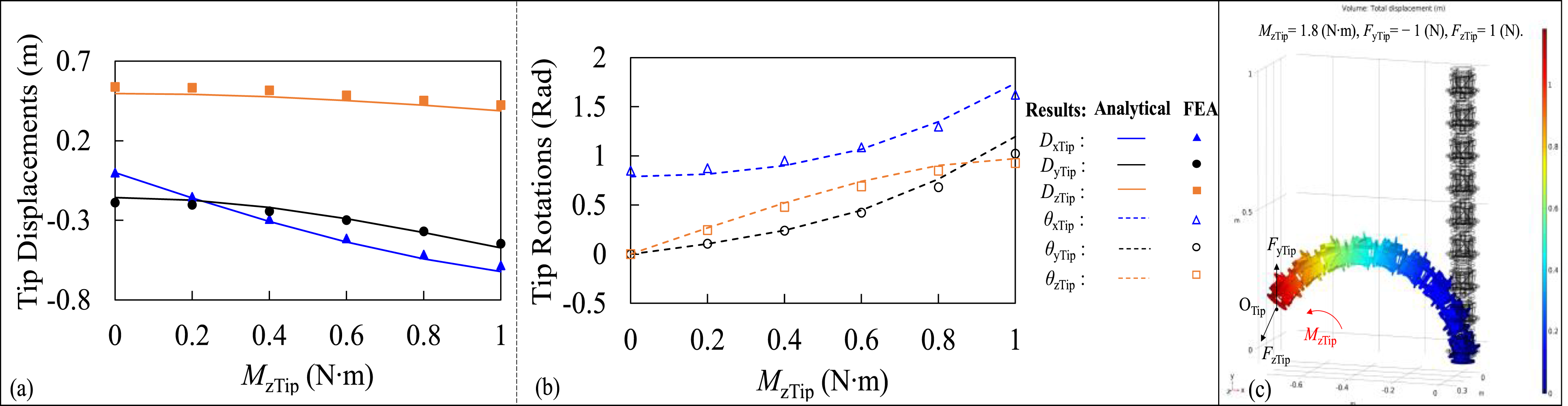
5.2. Tip-location accuracy and shape dexterity
We vary the cable forces to evaluate the “L” and “S” shapes of the three-segment ACCR. (1) “L” shape
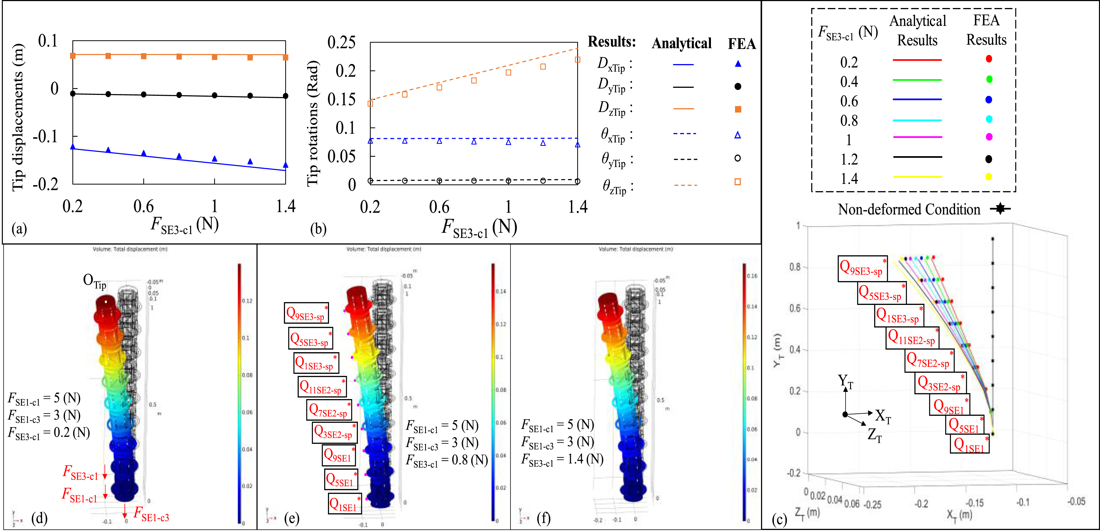
The cable forces FSE1-c1 = 5 (N), FSE1-c3 = 3 (N), and FSE3-c1 range from 0.2 (N) to 1.4 (N) with a step of 0.2 (N), and other cable forces are equal to 0, as shown in Figure 13(d). The cable-force components loading at Q1SE1, Q5SE1, and Q9SE1 due to FSE1-c1, cable-force components loading at Q3SE1, Q7SE1, and Q11SE1 due to FSE1-c3, and cable-force components loading at Q1SE3, Q5SE3, Q9SE3, Q1S3S2, Q5S3S2, Q9S3S2, Q1S3S1, Q5S3S1, and Q9S3S1 due to FSE3-c1 can be solved in the analytical model (as seen in Figure 4), which are substituted into the FEA model. The FEA (2) “S” shape “L” shape of the three-segment ACCR with respect to OT-XTYTZT: (a) tip displacements, (b) tip rotations, (c) shape dexterity with the increase of FSE3-c1, (d) the total displacement under FSE3-c1 = 0.2 (N), (e) the total displacement under FSE3-c1 = 0.8 (N), and (f) the total displacement under FSE3-c1 = 1.4 (N). The average differences between the analytical results and their corresponding FEA results: DxTip: 5.5%, DyTip: 8.3%, DzTip: 5.9%, θxTip: 6.0%, θyTip: 8.5%, and θzTip: 5.3%. The average differences of the coordinates between the analytical and FEA ACCR shapes in Figure 13(c) with respect to XT, YT, and ZT axes are 2.2%, 0.1%, and 6.2%, respectively).
The cable forces: FSE1-c1 ranges from 0 (N) to 5 (N) with a step of 1 (N), FSE1-c3 = 2 (N), FSE3-c2 = 1.2 (N), an d other cable forces are equal to 0. The cable-force components loading at Q1SE1, Q5SE1, and Q9SE1 due to FSE1-c1, the cable-force components loading at Q3SE1, Q7SE1, and Q11SE1 due to FSE1-c3, and the cable-force components loading at Q2SE3, Q6SE3, Q10SE3, Q2S3S2, Q6S3S2, Q10S3S2, Q2S3S1, Q6S3S1, and Q10S3S1 due to FSE3-c2 can be solved in the analytical model, which are substituted into the FEA model. Tip displacements and rotations of the FEA and nonlinear kinetostatic models are compared in Figure 14(a) and (b). “S” shape with the increasing of FSE1-c1 is shown in Figure 14(c)–(j). “S” shape of the three-segment ACCR with respect to OT-XTYTZT: (a) tip displacements, (b) tip rotations, (c) shape dexterity with the increase of FSE1-c1, (d) total displacement when FSE1-c1 = 0 (N), and (e) total displacement when FSE1-c1 = 5 (N). The average differences between the analytical results and their corresponding FEA results: DxTip: 5.1%, DyTip: 8.1%, DzTip: 5.4%, θxTip: 6.0%, θyTip: 7.9%, and θzTip: 2.7%. The average differences of the coordinates between the analytical and FEA ACCR shapes in Figure 14(c) with respect to XT, YT, and ZT axes are 0.52%, 0.05%, and 6.3%, respectively).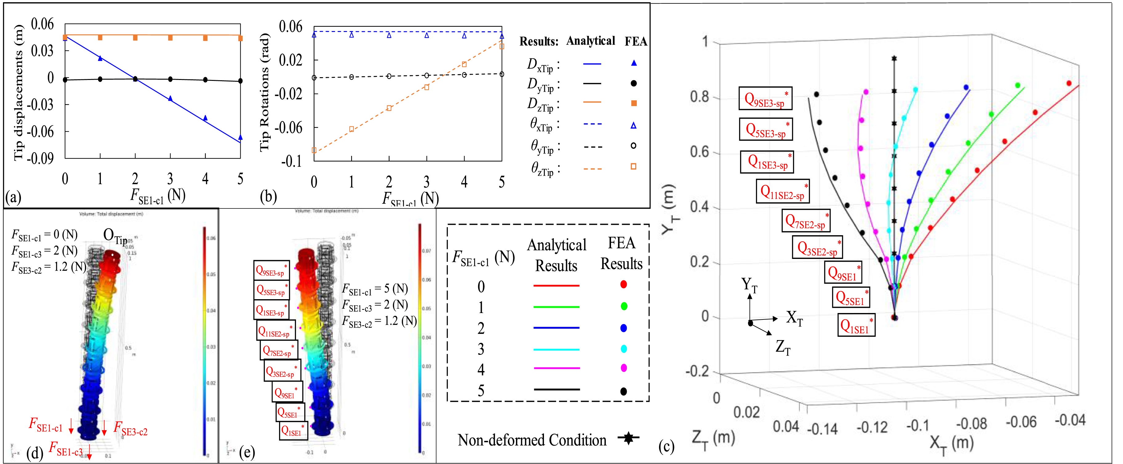
5.3. Tip-stiffness improvement
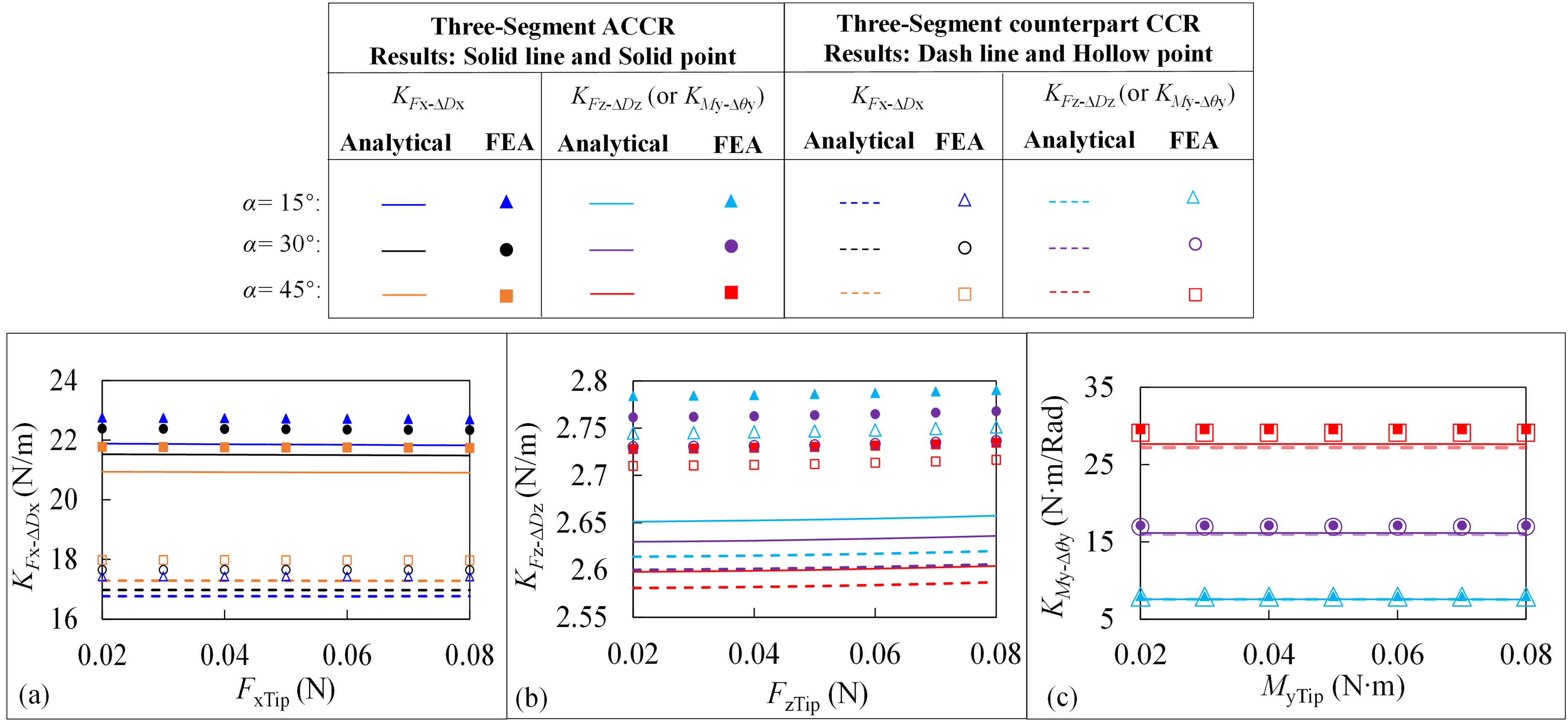
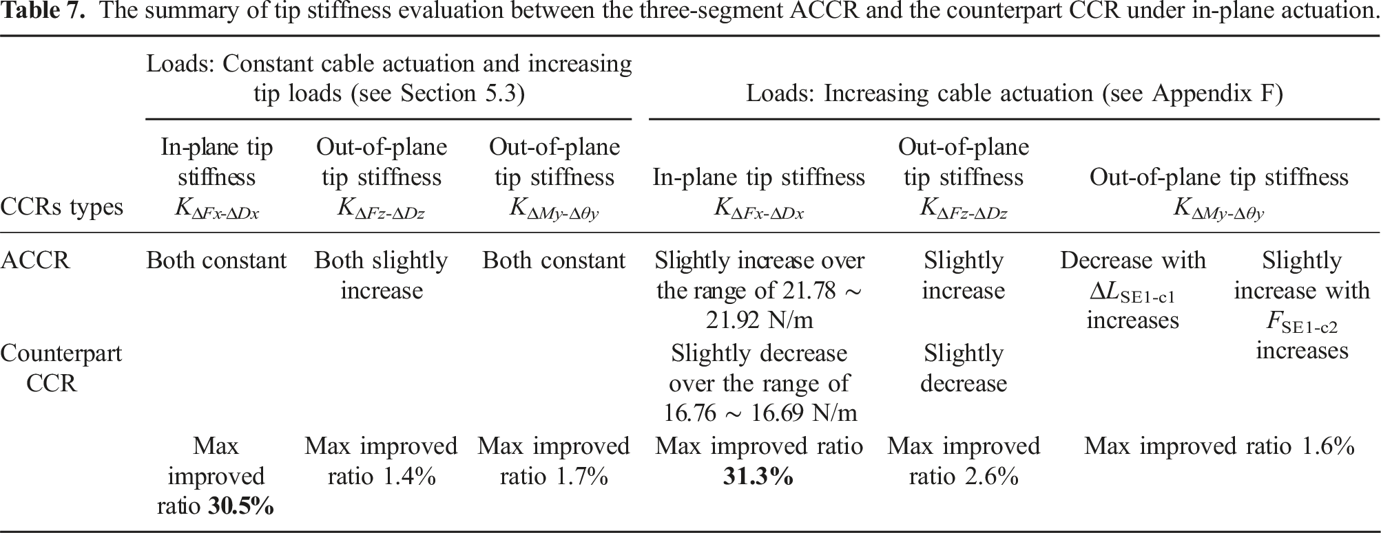
Similar to Section 4.3, the tip stiffness of the three-segment ACCR and the counterpart CCR are compared. The two three-segment CCRs have the same geometric parameters and cables are located at the level of the sheets’ free ends. λ takes 0.5, α = 15°, 30°, or 45°, and the loading condition is an increasing tip load with constant cable-displacement actuation. ∆LSE1-c1 = 6 (mm) and ∆LSE3-c2 = − 2 (mm), which means that LSE1-c1 is pulled down by 6 (mm) and LSE3-c2 is elongated by 2 (mm). Other cables are free. These loading conditions are held in the following three situations. (i) To compare the in-plane tip stiffness K∆Fx-∆Dx of the ACCR and counterpart CCR, the in-plane tip load FxTip ranges from 0.02 to 0.08 (N) with a step of 0.02 (N). Their results are shown in Figure 15(a). The maximum difference between the analytical and FEA results is 5.2%. K∆Fx-∆Dx_ACCR has high values under a small α, which is the highest under α = 15°. However, K∆Fx-∆Dx_coun has low values under a small α, which is the smallest under α = 15°. K∆Fx-∆Dx_ACCR is larger than K∆Fx-∆Dx_coun, and K∆Fx-∆Dx_ACCR under α = 15°, 30° or 45° increases by 30.5%, 26.8%, and 21.1%, respectively. (ii) To compare the out-of-plane tip stiffness K∆Fz-∆Dz of the ACCR and counterpart CCR, the out-of-plane tip load FzTip ranges from 0.02 to 0.08 (N) with a step of 0.02 (N). Their results are shown in Figure 15(b). The maximum difference between the analytical and FEA results is 6.5%. K∆Fz-∆Dz of the two CCRs both have high values under a small α. K∆Fz-∆Dz of the two CCRs are close but K∆Fz-∆Dz_ACCR is slightly larger than K∆Fz-∆Dz_coun under the same geometric parameters and loading conditions. K∆Fz-∆Dz_ACCR under α = 15°, 30° or 45° increases by 1.4%, 1.1%, and 0.7%, respectively. (iii) To compare the out-of-plane tip stiffness K∆My-∆θy of the ACCR and counterpart CCR, the tip twisting moment MyTip ranges from 0.02 to 0.08 (N) with a step of 0.02 (N). Their results are shown in Figure 15(c). The maximum difference between the analytical and FEA results is 7.2%. K∆My-∆θy of the two CCRs have high values under a big α, which means K∆My-∆θy is the largest under α = 45°. K∆My-∆θy_ACCR is slightly higher than K∆My-∆θy_coun under the same geometric parameters, where K∆My-∆θy_ACCR and K∆My-∆θy_coun denote the K∆My-∆θy of the ACCR and counterpart CCR, respectively. K∆My-∆θy_ACCR under α = 15°, 30° or 45° increases by 0.5%, 1.1%, and 1.7%, respectively. The effects of α and tip loads on the tip stiffness of the three-segment CCRs are in line with those of the one-segment CCRs. The in-plane and out-of-plane tip stiffness comparison between the three-segment ACCR and the counterpart CCR under a constant cable-displacement actuation: (a) the in-plane tip stiffness K∆Fx-∆Dx under a series of increasing FxTip, (b) the out-of-plane tip stiffness K∆Fz-∆Dz under a series of increasing FzTip, and (c) the out-of-plane tip stiffness K∆My-∆θy under a series of increasing MyTip.
The summary of tip stiffness evaluation between the three-segment ACCR and the counterpart CCR under in-plane actuation.
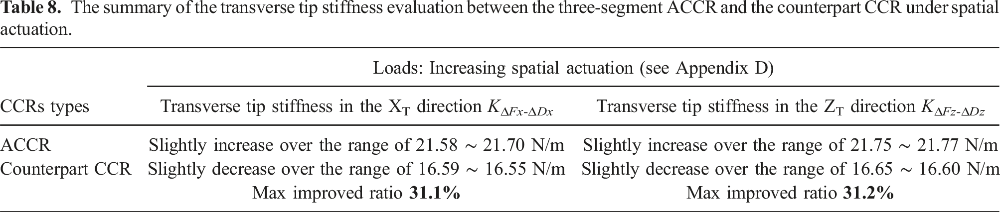
The summary of the transverse tip stiffness evaluation between the three-segment ACCR and the counterpart CCR under spatial actuation.
5.4. Experiments
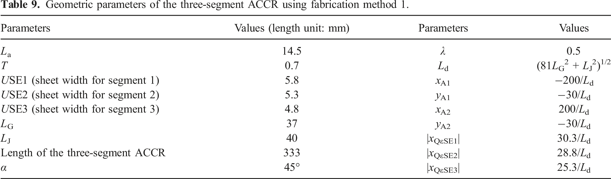
We experimentally test a three-segment ACCR prototype under planar actuation, aiming to assess its manufacturability and validate the proposed analytical model across various scenarios. In Figure 16, the prototype of an ACCR using fabrication method 1. (For more details on fabrication, Appendix E can be visited). The corresponding parameters of the prototype are shown in Table 9. All modular units have identical rigid structures, differing only in sheet width. Each anti-buckling universal joint has a weight of close to 22 (g). Fabricated modular unit and the ACCR: (a) modular unit, (b) modular units of segments 1, 2, and 3, (c) three segments, and (d) ACCR prototype with cables. Geometric parameters of the three-segment ACCR using fabrication method 1.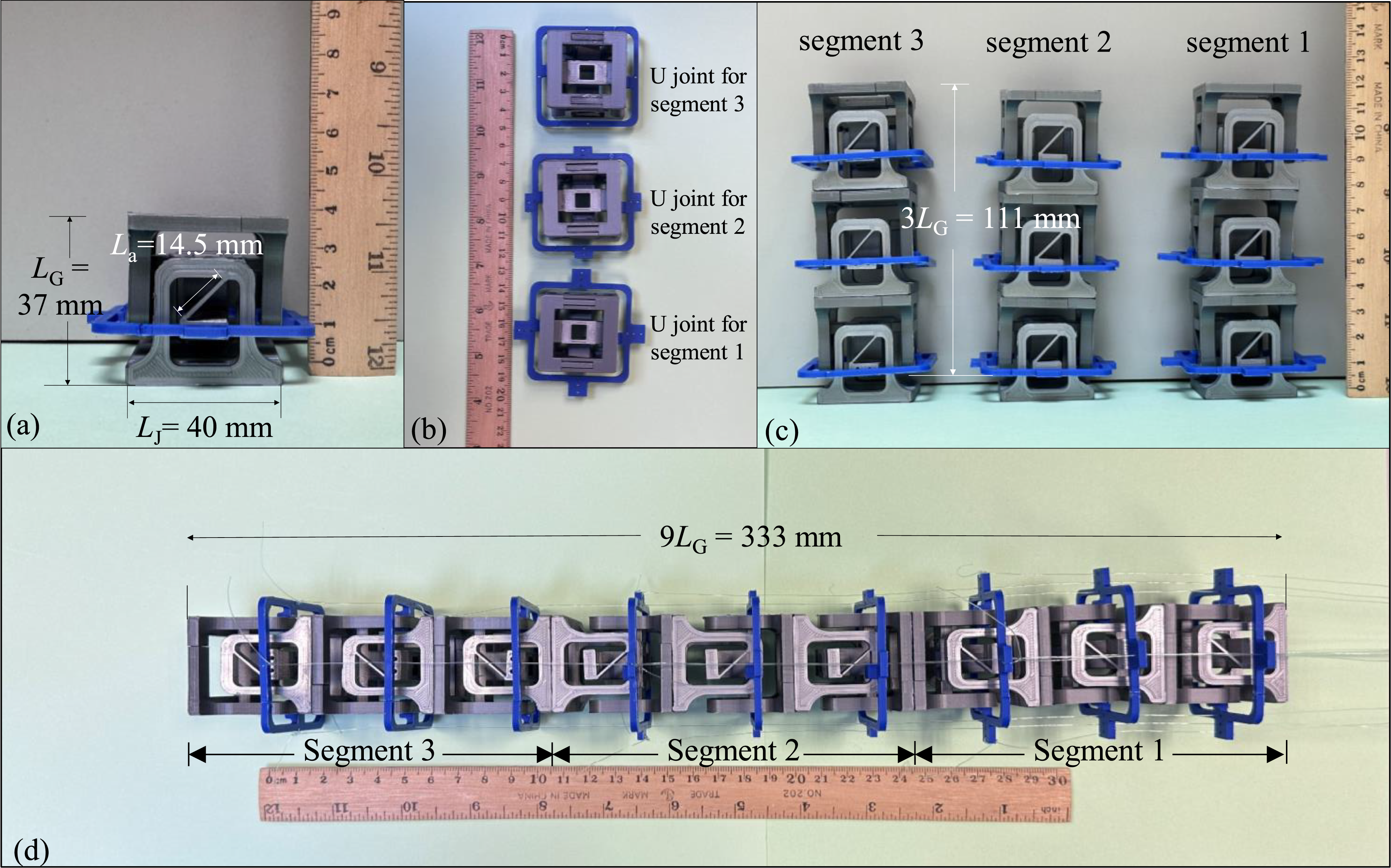
During the experiments, we observed that segment 1 helps to resist unwanted deformations when large forces are applied at the tip. The more flexible segment 3 allows for finer, more dexterous movements, making it ideal for precise positioning. The gradual transition in stiffness creates smoother flexibility variations, enhancing the ACCR’s overall performance in kinetostatic tasks. Three performance indicators, tip displacements, tip trajectory, and tip stiffness are used to evaluate the prototype. The test setup is shown in Figure 17(a). The base of the prototype is fixed on the working bench, and the three-segment ACCR is placed in an upside down position to eliminate the gravity effect in the non-deformed shape. We use different weights to provide cable forces, as shown in Figure 17(b) and (c). The tip displacements can be calculated by counting the number of squares in the graph paper, as shown in Figure 17(d). Experiments of the three-segment ACCR: (a) no-loads acting on the ACCR, (b) the weight of FSE1-c2 is 40 g, (c) the weight of FSE1-c2 is 40 g and the weight of FSE3-c2 is 100 g, and (d) the double exposure of Figs. 17(b) and (c) for calculating tip displacements. (Note that “double exposure” typically refers to a photographic technique where two images are combined into a single frame, creating a layered or blended effect).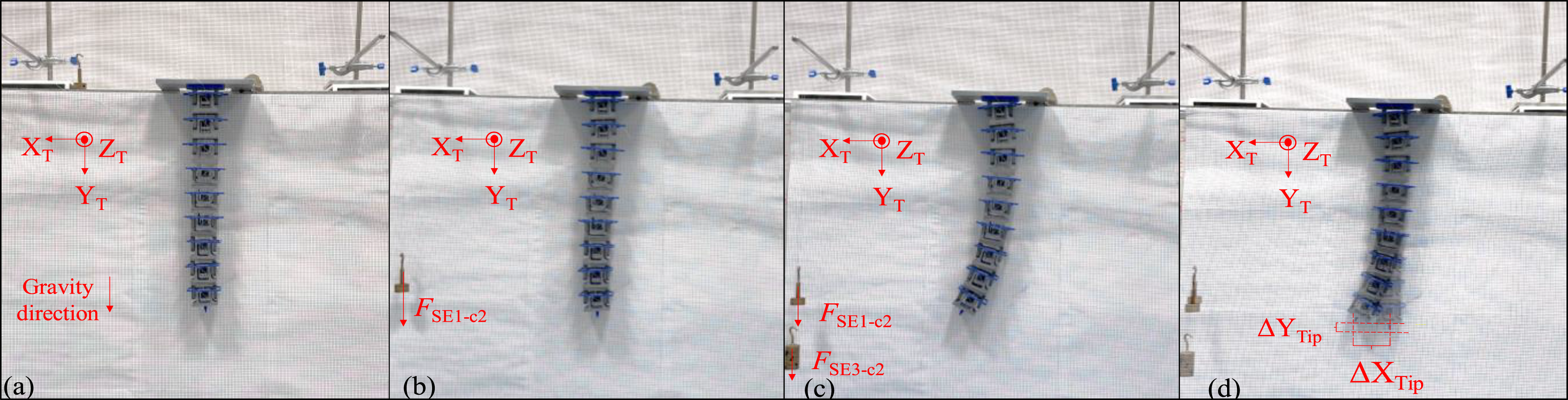
The L shape of the three-segment ACCR is tested first, as shown in Figure 18(a). The weight that provides the cable force FSE1-c2 is constant at 40 (g). The weights that provide the cable force FSE3-c2 range from 0 (g) to 100 (g) with a step of 20 (g). The analytical and experimental results are compared in Figure 18(b) and (c), and the average differences of DxTip and DyTip are 4.5% and 5.5%, respectively. L shape test of the three-segment ACCR: (a) tip displacement with loads, (b) tip displacements DxTip and DyTip, and (c) tip trajectory of the tip marker.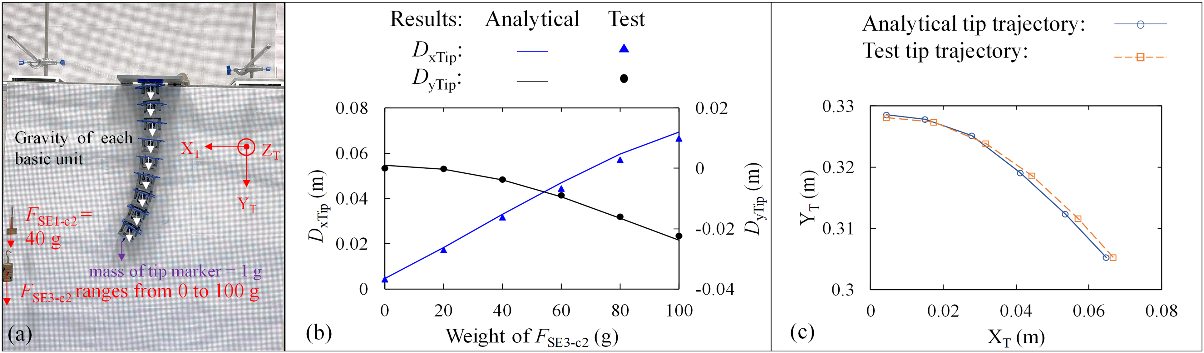
The S shape of the three-segment ACCR is tested as shown in Figure 19(a). The weight that provides the cable force FSE1-c2 is constant at 100 (g). The weights that give the cable force FSE3-c1 range from 0 (g) to 100 (g) with a step of 20 (g). The analytical and experimental results are compared in Figure 19(b) and (c), and the average differences of DxTip and DyTip are 5.3% and 4.6%, respectively. S shape test of the three-segment ACCR: (a) loading conditions, (b) tip displacements DxTip and DyTip, and (c) tip trajectory of the tip marker.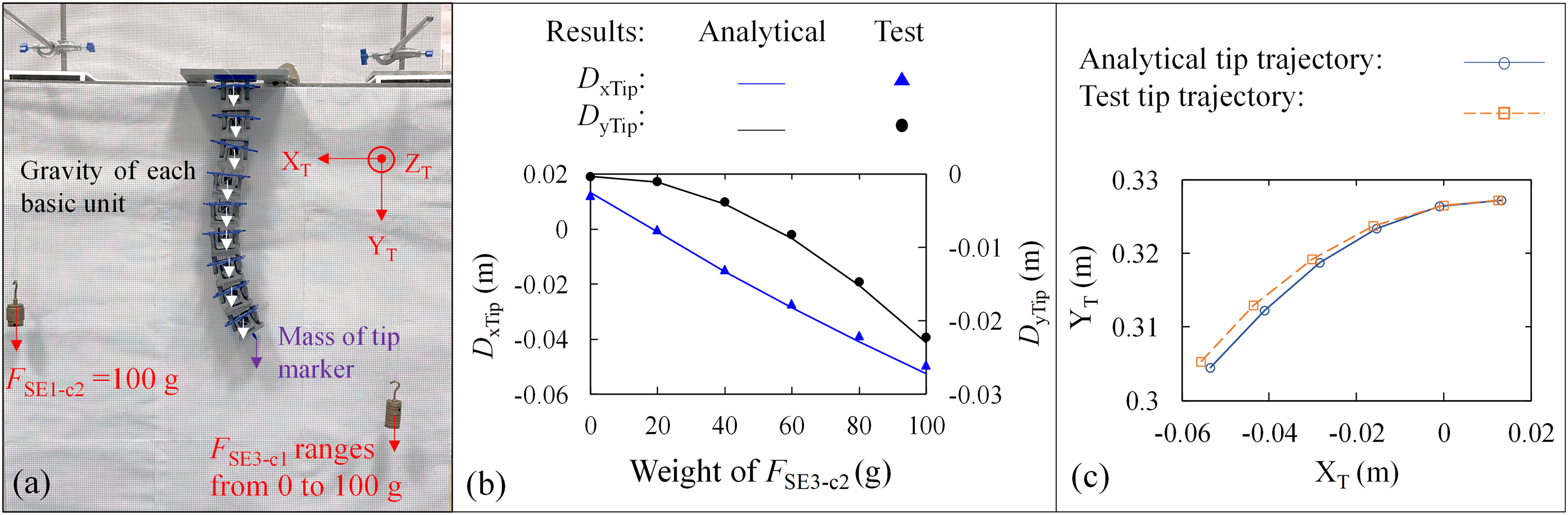
The tip stiffness is also evaluated as shown in Figure 20. Two cable displacements are constant, and other cables are free. ΔLSE1-c1 = 6 (mm) and ΔLSE3-c2 = 4 (mm). The cable displacement is adjusted by a 3D printing cylinder. The cylinder diameter is 1/π. Each time the cable wraps around the cylinder, and it pulls by 1 mm. The weight that provided tip force along the XT-axis increases from 0 to 70 (g) with a step of 10 (g). The analytical and experimental results are compared in Figure 20(b)–(d), and the average differences of DxTip, DyTip, and KΔFx-Δx are 5.5%, 4.6%, and 5.07%, respectively. KΔFx-Δx increases significantly with the increase of FxTip, as described in Figure 20(d). This is because the minimum available weight in the test is 10 (g), causing a much larger increment over the increase of FxTip. The tip stiffness test of the three-segment ACCR: (a) loading conditions, (b) tip displacements DxTip and DyTip, (c) the tip trajectory of the tip marker, and (d) the tip stiffness increases with FxTip under constant cable displacements.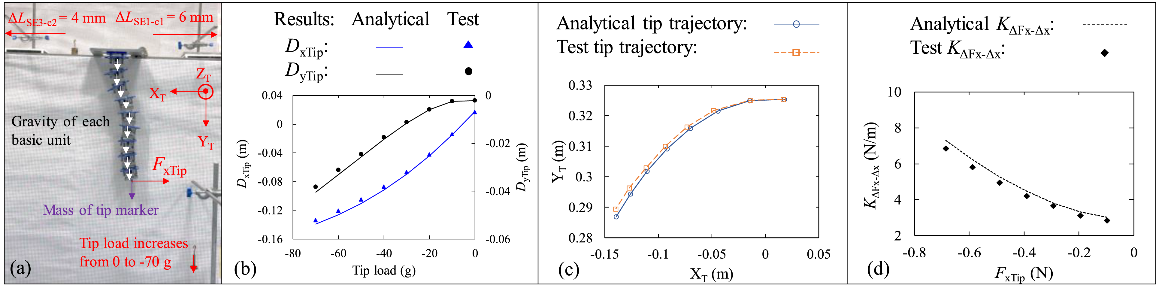
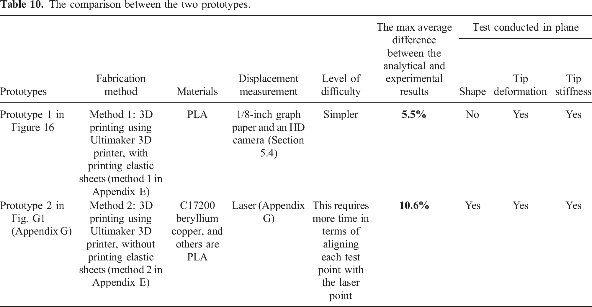
The comparison between the two prototypes.
Although experimental results of the three-segment CCRs under increasing cable actuation were not obtained, the analytical results in both FEA and analytical modeling show that the tip stiffness can be increased by increasing the cable force or displacements for the ACCR, which can be seen in Figure 2(c) and (d) of Appendix F.
6. Remarks of the ACCR
Any dominant loads/displacements acting on the CCR have been considered in the proposed kinetostatic model (such as cable forces, prescribed cable actuation displacements, tip loads, and gravity), and their effects on the CCR’s performances have been evaluated in Sections 4 and 5. In this section, we will discuss many aspects of the analytical model and the ACCR including the gravity effect, unaccounted considerations, fabrication scalability, reliability, and the comparison with other existing designs.
6.1. Gravity effect
The gravity effect has been included in the analytical, experimental, and FEA models. The gravity effect on the ACCR depends on the application environment and ACCR’s placements. For example, the gravity of the ACCR has less influence on its deformation when it is utilized in underwater or space. This section discusses how gravity influences the shape dexterity of the three-segment ACCR, when it is placed upside down, upright, or horizontally under a constant cable-force actuation and a tip load. FSE1-c1 = 3 (N), FSE3-c2 = 0.3 (N) and FzTip = 0.1 (N). We assume that the mass of each anti-buckling is 20 (g), and the gravity of each anti-buckling universal joint is located at its rotational center. λ = 0.5 and α = 15° here and other geometric parameters are the same as those of Section 5.1.
Figure 21(a) describes the FEA model of the three-segment ACCR under λ = 0.5 and α = 15°. Figure 21(b) and (c) show the shape dexterity through XTYT and YTZT planes, respectively. The maximum difference between the analytical and FEA results is 3.4%. When the ACCR is placed upside down and upright, the gravity of each anti-buckling universal joint is along the positive and negative direction of the YT-axis, respectively, as given in Figure 21(e) and (f). The analytical model in Section 3.2 can be used directly. When the ACCR is placed horizontally, the gravity of each anti-buckling universal joint is along the positive direction of the XT-axis, as shown in Figure 21(g). The gravity-related equation should be revised, such as equation (39), [0, fmaJΩSE3_T, 0, Gravity effect on the three-segment ACCR that is placed upside down, upright, or placed horizontally under the same actuation conditions. (a) Three-segment ACCR under λ = 0.5 and α = 15°, (b) shape dexterity through the XY plane, (c) shape dexterity through the YZ plane; the FEA total displacements when the ACCR is (d) no gravity, (e) placed upside down, (f) placed upright, and (g) placed horizontally.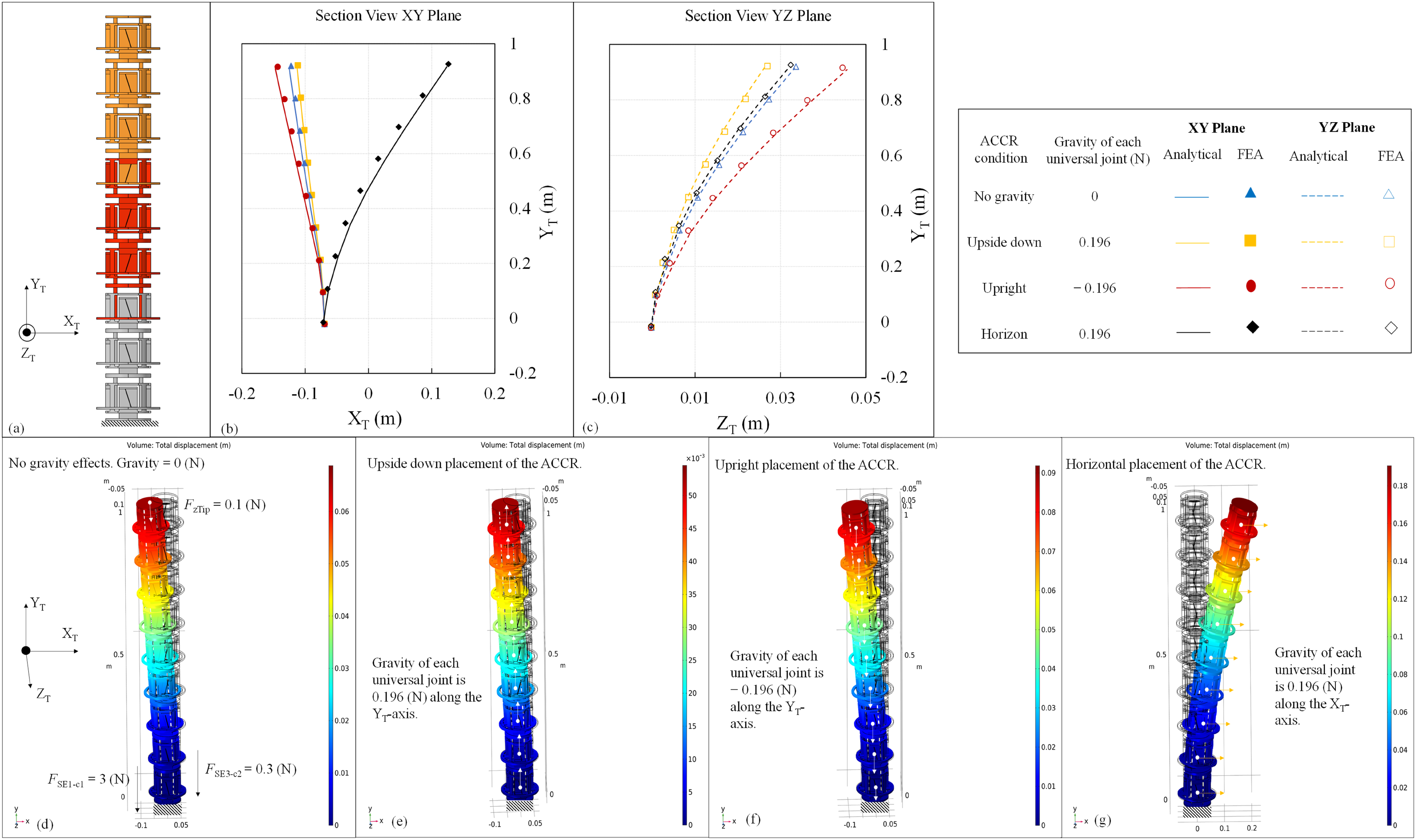
6.2. Unaccounted considerations in modeling of the ACCR
Friction (Roy et al., 2017), elongation and creep of cables (J. Li et al., 2020a), slack and hysteresis of cables, hysteresis of ACCR’s material, temperature (Kim et al., 2017), and dynamics (Z. Liu et al., 2021), are common factors influencing the performance of robot. In this section, their effects on the ACCR’s performance are discussed. (1) Friction
Compliant joints do not introduce any friction. The source of friction in the continuum robot system is mainly due to the contact between the cables and the holes, which can increase the actuation forces slightly (i.e., actuation stiffness increase). Note we use Clear Nylon Fishing Wire (Eruinfang) as the actuation cable for the experiment, which is very smooth for making trivial contribution to influence our analytical model. The experimental displacement results are often slightly larger than the analytical models (i.e., actuation compliance increase) due to two reasons: i) the deformation of rigid parts is neglected in the proposed kinetostatic model and ii) the inevitable stiffness loss due to assembly. The above two effects can usually cancel out each other to make the experimental model agree with the analytical model. (2) Elongation and creep of cables
We did not consider cable elongation in the proposed analytical model. Dyneema thread is an ideal choice for a cable-driven ACCR. The cable break load and the Young’s modulus of a Փ0.4 (mm) Dyneema thread is 50 (kg) and at least 109 (GPa) (Sanborn et al., 2015), respectively. The Dyneema thread is of high strength, low density, and low elongation at break, making it highly suitable for the ACCR that demands substantial actuation forces. However, in our experiment, we used an alternative Փ0.4 (mm) Clear Nylon Fishing Wire (Eruinfang) as the actuation cable. The Young’s modulus of nylon is at least 2.7 (GPa). Our maximum actuation force is less than 0.1 (kg) in the experiment (due to the low stiffness of 3D printed joints), far below the cable break load (12.97 (kg)). So the elongation is not significant to affect the agreement between the analytical models and the experimental results as seen in Figures 18–20. (3) Slack and hysteresis of cables
The effects of cable slack and hysteresis on the ACCR’s repeatability are not studied in this paper. These effects will be investigated in our future experiments including cyclic loading tests, drift analysis over extended operation, feedback control, or tension monitoring systems. We will develop a more robust control strategy that compensates for these effects in real-time. (4) Hysteresis of ACCR’s material
The anti-buckling universal joints are fabricated from PLA. While polymers do exhibit some degree of creep under sustained stress, the impact on the ACCR depends on factors such as load magnitude, duration, and temperature. Creep in PLA is likely to occur when the material is under continuous mechanical stress, especially at temperatures approaching or exceeding its glass transition temperature (∼55 °C–65 °C). When we did the experiment, the ACCR was operated in a room temperature at about (22°C–23°C) during a short time. We also designed a limiter for the ACCR, which limits further deformation under heavy loads, providing additional protection.
We are planning further experiments to quantify the long-term impact of material creep on joint performance and to explore possible mitigation strategies, such as optimizing joint design. This will help us to ensure reliable performance in practical applications. Overall, while the material’s hysteresis and creep effects are present, our prototype exhibits acceptable for the ACCR’s intended tasks. (5) Temperature variations
In this paper, we did not investigate the effect of temperature variations on the performance of the ACCR. In our design and experiment, we did not apply materials that are sensitive to temperature variations, such as shape memory alloys, and we conducted our experiment in room temperature. Thus, the temperature variations on the performance of the proposed robot are not considered in this paper. However, if the ACCR is used in extreme temperature environments, such temperature effects should be modeled and tested, which is out of the scope of this paper.
(6) Dynamics
Continuum robots in real-world applications are often used for slow movements as shown in (Chen et al., 2021; Dong et al., 2015, 2019; Kang et al., 2017; K. Xu et al., 2015; K. Xu and Simaan, 2008), which has motivated us focus on the kinetostatic modeling and analysis as presented in this paper. We plan to develop a more comprehensive control system and method based on the proposed kinetostatic modeling approach. In addition, even without considering the velocity and acceleration contributions, a slow control (Abdelaziz et al., 2011) can be conducted where inertia and damping are not considered.
6.3. Scalability
Two methods using a low-cost Ultimaker 3D printer have been proposed in this paper for fabricating two assembled prototypes. A small-scale modular unit with a diameter of 40 mm and a height of 37 mm has been shown in Figure 16. As a comparison, a large-scale anti-buckling universal joint, with a diameter of 110 mm and a height 87 mm, is also presented in (S. Li and Hao, 2022).
We believe that the limiting factors to a miniaturized CCR would be the capability of the used 3D printer and/or the assembly of the small parts. The biggest hurdle to further increase the size of the robot system would be the significant gravity effect due to the heavy mass introduced, which can increase the actuation effort and control complexity (due to cable pretension). The mass of the CRR can be considered an important parameter in our analytical model, as described in Section 6.1. The scale (such as how large it is possible) of the robot system is also dependent on an actual application (with desired specific performances). For example, for the human-machine collaboration, a large-scale ACCR alike a human arm would be desired.
Thus, mass, assembly methods, segment numbers, cable distributions/numbers, and geometric parameters are all influencing factors that contribute to both the scale and the performances of the ACCR.
6.4. Reliability
A reliable CCR can perform its tasks consistently, safely, and efficiently, while avoiding breakdowns, errors, and failures. The reliability of the ACCR is discussed in light of breakdown possibility and motion accuracy. (1) Breakdown possibility
The breakdown possibility of the ACCR mainly depends on the properties of elastic sheets. The ratio of flexure strength to Young’s modulus of the elastic sheets is large, which decreases the possibility of breakdown. What’s more, the ACCR is designed for the use in a low-cycle application to avoid fatigue. Throughout the deformation evaluation in this paper, the max von Mise stress obtained by FEA of the ACCR is always far less than the yield stress. (2) Motion accuracy
Validation of the three-segment ACCR in accommodating manufacturing or fabrication errors.
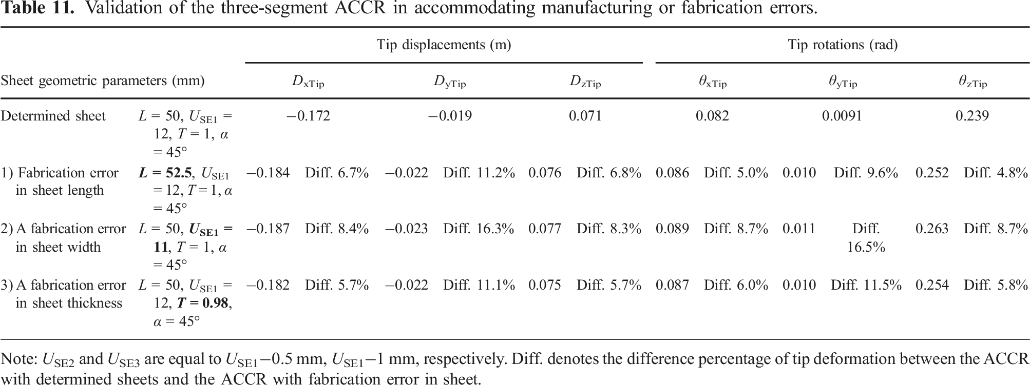
Note: USE2 and USE3 are equal to USE1−0.5 mm, USE1−1 mm, respectively. Diff. denotes the difference percentage of tip deformation between the ACCR with determined sheets and the ACCR with fabrication error in sheet.
6.5. Comparison with existing representative work
In this section, we summarize the comparisons between the ACCR and existing CCRs from three aspects, including working principle of increasing stiffness, analytical model, and other characteristics.
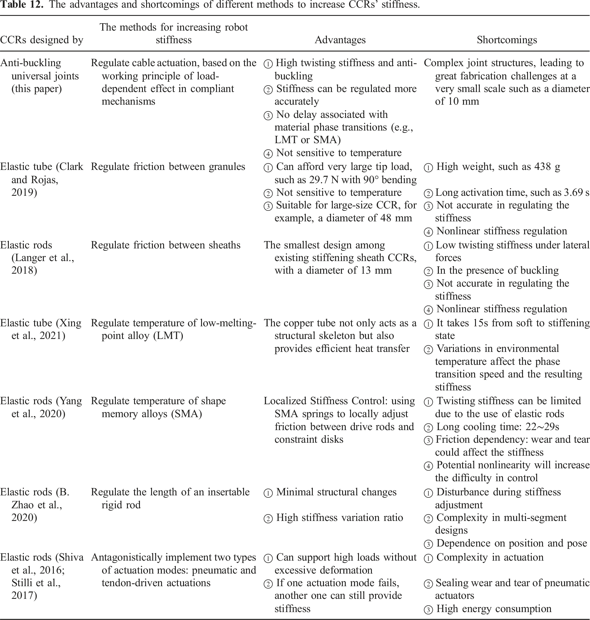
The advantages and shortcomings of different methods to increase CCRs’ stiffness.
The proposed analytical model is based on the spatial nonlinear beam constraint model (BCM) and free-body diagram. Table 13 summarizes the advantages and shortcomings of the proposed analytical model and existing analytical models. The proposed analytical model has three key advantages over existing analytical models. (1) The proposed analytical model accounts for localized, discrete, and distributed loads, whereas other analytical models have limitations in handling these types of loads. The advantages and shortcomings of the proposed analytical model and existing analytical models.
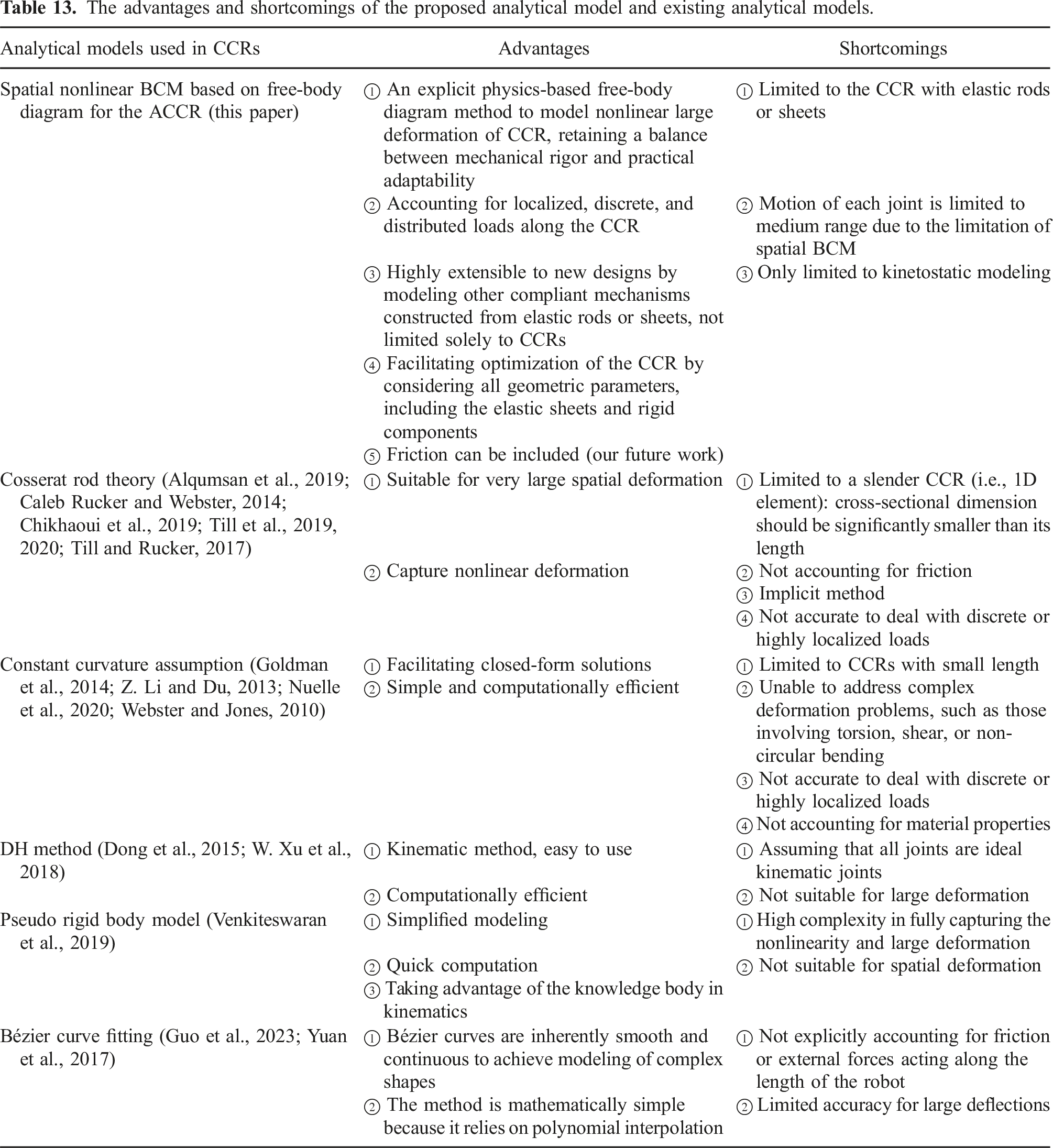
Many practical engineering applications, especially those involving tendon-driven robots, do not fit neatly into a purely distributed-loading framework. Instead, localized or discrete loads often occur, such as contact forces and friction at cable-routing holes or pivot joints. The proposed analytical model directly captures localized interactions without forcing them into a distributed framework. Each contact interface (e.g., a cable-routing hole) can be treated as an individual node. This preserves the true mechanical behavior at each interface and allows any force or moment to be precisely calculated from fundamental laws of equilibrium. For example, cables pass through all the holes along the ACCR, and the forces applied by the cables at each hole are considered individually.
Constant curvature or polynomial-based models are widely used for CCRs primarily due to their simplicity in describing geometry. However, they often approximate distributed loads when non-tip loads act on CCRs, which can cause inaccuracies for discrete or highly localized loads. Cosserat Rod Theory is among the most comprehensive mathematical formalisms for describing continuum structures because it naturally captures distributed loads via continuous functions (e.g., f(s) for forces and m(s) for moments along the elastic rod, where s is the arc length). However, external forces and moments are usually treated as continuous distributions. When forces arise from discrete contacts, such as friction at a small interface, representing them as f(s) may involve artificial “spread-out” distributions or Dirac delta functions. (2) Shear and twisting deformations can be derived accurately by using the proposed analytical model, whereas other analytical models do not provide this level of accuracy or are limited to a stronger assumption, such as being slender CCRs for the Cosserat Rod Theory.
CCRs are designed to be highly flexible and deformable, often undergoing complex spatial motions that include shear, twisting, and bending. We use spatial BCM (Bai et al., 2021) to derive the proposed analytical model of the ACCR, which accounts for shear, twisting and bending deformations for each elastic sheet. Cosserat Rod Theory treats the entire CCR as multiple one-dimensional (1D) elements, so that the shear, twisting, and bending deformations along the CCR can be derived accurately. However, it is not ideal for capturing the shear and twisting of a CCR when its cross-sectional dimension is not significantly smaller than the CCR’s length. (3) The proposed analytical model makes the overall model highly extensible to new designs and optimizations, which is suitable for other compliant mechanisms constructed from elastic rods or sheets, not limited solely to CCRs.
Researchers can introduce or modify friction interfaces, cable-routing hole geometries, or internal mechanisms by simply incorporating them into the local free-body diagrams. In contrast, adapting Cosserat Rod Theory to capture such detailed physics might require substantial reformulation or extensive approximations. As such, the proposed model strikes a balance between mechanical rigor and ease of customization, aligning well with the design-oriented needs of advanced CCRs. The analytical model accounts for all design parameters of the CCR, including elastic sheets, rigid components, and cable-loading positions, along with material properties. These factors influence key performance characteristics of CCRs, such as tip stiffness, tip position, and shape dexterity. By optimizing these design parameters, the CCR can be tailored to meet specific application requirements.
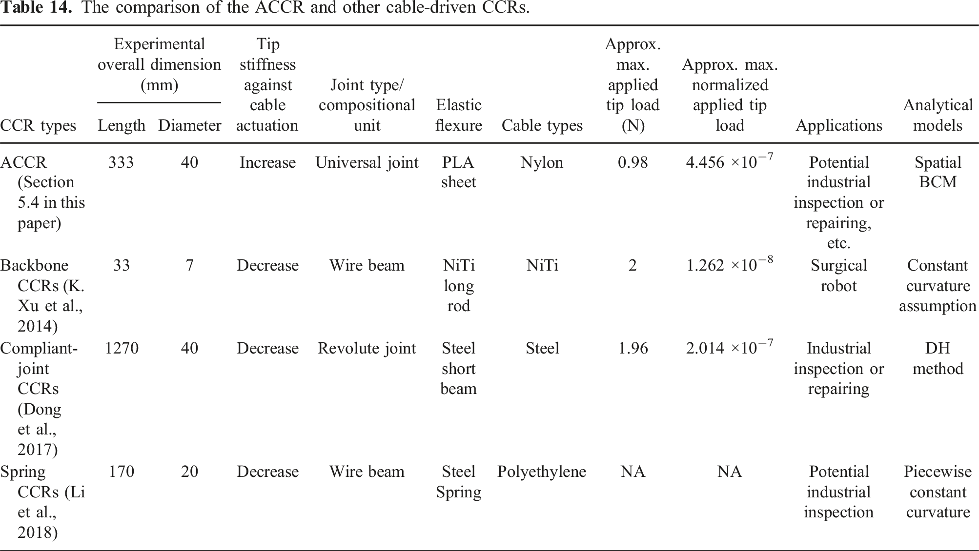
In this paper, the three-segment ACCR is physically developed in a medium size, targeting industrial applications. Its diameter and length are 40 (mm) and 333 (mm), respectively. The potential applications include industrial inspection and repairing (Dong et al., 2017) as well as human-machine integrated robotic systems (W. Liu et al., 2022). We applied the normalized tip loads to compare the tip load across scales. Normalized loads are dimensionless, which can account for material’s properties such as Young’s modulus and CCRs’ dimension, representing an appropriate normalized metric for cross-scale comparisons. We assume the CCR is an equivalent elastic beam and therefore, the maximum normalized tip load can be derived by using equation (53). The maximum tip load is defined based on the maximum deformation, just before buckling occurs.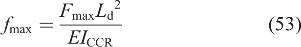
The comparison of the ACCR and other cable-driven CCRs.
7. Conclusions and future work
A tip stiffness improved cable-driven compliant continuum robot (ACCR) is proposed in this paper, which consists of multiple anti-buckling universal joints. The nonlinear spatial analytical models (i.e., forward kinetostatic models) of the ACCR have been derived under spatial loading conditions including cable-force actuation, cable-displacement actuation, tip loads, and gravity. One potential advantage of the proposed nonlinear analytical models is that any loads acting on the ACCR can be considered, and loads due to environmental constraints can be potentially considered in the analytical models if necessary. The proposed system modeling framework can be used to model other CCRs with different compliant joints. The maximum deformation, tip-location accuracy, shape dexterity, and tip stiffness of the ACCR have been comprehensively studied. The tip stiffness comparison between the ACCR and the counterpart CCR has been particularly investigated under two in-plane loading conditions, including (a) constant cable actuation, and (b) increasing cable actuation. The effect of geometric parameters, cable displacements, and cable forces on tip stiffness has been analyzed for the ACCR and the counterpart CCR. The tip stiffness of the one-segment ACCR and that of the counterpart CCR have been compared in experimental tests. The tip displacement, tip trajectory and tip stiffness of the three-segment ACCR have been experimentally evaluated.
The main results are summarized as follows. (1) The proposed nonlinear analytical models have a high accuracy compared with FEA models when each anti-buckling universal joint has an intermediate range of motion. The maximum difference between the analytical and FEA results is less than 7% except for those results of very small axial displacements and twisting rotations. The maximum difference between the analytical and experimental results is less than 6%. (2) Our design can produce high bending curvatures and variable shapes, whose motions in the DoC directions are well-constrained, such as twisting motions. (3) The tip stiffness of the ACCR is always higher than that of the counterpart CCR under α ≤ 45° with any λ, when they are under the same geometric parameters and loading conditions. Therefore, ACCR enables a slenderer shape and higher tip stiffness than the counterpart CCR. (4) Effects of geometric parameters and loading conditions on the tip stiffness of the one-segment and three-segment CCRs under increasing in-plane actuation have been summarized in Table 4 and Table 7, respectively, which are also briefly presented below. (a) The in-plane tip stiffness of the ACCR increases with the increase of cable forces or displacements, and the tip stiffness change range is larger. However, the in-plane tip stiffness of the counterpart CCR decreases with the increase of cable forces or displacements. (b) The out-of-plane tip stiffness (due to the out-of-plane tip forces) of the ACCR slightly increases with the increase of cable forces or displacements. However, the out-of-plane tip stiffness of the counterpart CCR has the opposite trend. (c) The out-of-plane tip stiffness (due to the twisting tip moments) of the ACCR and that of the counterpart CCR all decreases with the increase of cable displacements while slightly increasing with the increase of cable forces. (5) When the ACCR and the counterpart CCR are all under increasing spatial actuation, all the transverse tip stiffness of the ACCR can increase. Their results are summarized in Table 5 and Table 8 in Appendix D. (6) The one-segment CCR experimental results validate that a) ACCR’s stiffness is much larger than that of the counterpart CCR; b) the ACCR tip stiffness can increase by increasing actuation forces. The three-segment CCR experimental results validate that a) the proposed analytical model has a high accuracy for predicting tip trajectory and various body shapes; b) the tip stiffness increases with the increase of tip forces.
In the future, the design parameters of the ACCR will be optimized so that the tip stiffness of the ACCR can increase more significantly by increasing the cable actuation. We will build a comprehensive control system for the ACCR. The actuation, sensing, and motion/force control of the ACCR will be investigated by developing both hardware and associated software/algorithms. Leveraging the advantages of the kinetostatic modeling method, we will explore the crucial intrinsic ability to detect contact locations and interaction forces between the ACCR and its environment. In addition, we will carry out a series of experiments on the unaccounted considerations in modeling of the ACCR. across various scenarios.
Supplemental Material
Supplemental Material - Design and kinetostatic analysis of a tip-stiffness improved compliant continuum robot using anti-buckling universal joints
Supplemental Material for Design and kinetostatic analysis of a tip-stiffness improved compliant continuum robot using anti-buckling universal joints by Shiyao Li, Salih Abdelaziz, Long Wang, and Guangbo Hao in The International Journal of Robotics Research
Footnotes
Acknowledgments
The authors would like to sincerely thank Siyuan Ye and Kong Zhang for their help in the fabrication and testing of the prototypes. The authors appreciate Mr Timothy Power and Mr Michael O’Shea for their excellent fabrication work. Shiyao Li is funded by the China Scholarship Council.
Declaration of conflicting interests
The author(s) declared no potential conflicts of interest with respect to the research, authorship, and/or publication of this article.
Funding
Shiyao Li is funded by the China Scholarship Council (201806440050).
Supplemental Material
Supplemental material for this article is available online.
References
Supplementary Material
Please find the following supplemental material available below.
For Open Access articles published under a Creative Commons License, all supplemental material carries the same license as the article it is associated with.
For non-Open Access articles published, all supplemental material carries a non-exclusive license, and permission requests for re-use of supplemental material or any part of supplemental material shall be sent directly to the copyright owner as specified in the copyright notice associated with the article.