Physics-informed robotic airflow exploration and mapping with a swarm of mobile robots

Abstract

Airflow is the key transport mechanism for airborne substances like gas or particulate matter. It is of great interest in many applications ranging from evacuation planning to analyzing indoor ventilation systems. However, accurately determining a spatial map of the airflow is difficult and time-consuming since environmental parameters and boundary conditions are often unknown. This work introduces a novel adaptive sampling strategy for mobile robots. The strategy allows multiple mobile robots with anemometers to autonomously collect airflow measurements and generate a two-dimensional spatial map of the airflow field. Using a Domain-knowledge Assisted Exploration approach, the robots respond in real-time to the measurements already taken and determine the most informative locations online for further measurements. We incorporate the Navier-Stokes Partial Differential Equations to fuse the collected data with model assumptions. By casting the airflow model into a probabilistic framework, we can quantify uncertainties in the airflow field and develop an intelligent, uncertainty-driven exploration strategy inspired by optimal experimental design principles. This strategy combines an estimated uncertainty map with a rapidly exploring random tree path planner. Additionally, using the Navier-Stokes equations allows us to interpolate spatially between measurements in a physics-informed way, enabling us to construct a more accurate airflow map. We implemented and evaluated the proposed concept in simulations and experiments in a laboratory environment, where five mobile robots explore artificially generated airflow fields. The results indicate that our approach can correctly estimate the airflow and show that the proposed adaptive exploration strategy gathers information more efficiently than a predefined sampling pattern.

1. Introduction

In many practical problems in engineering that are concerned with analyzing the dispersion of airborne substances, an accurate representation of airflow is of key importance: airflow is often the dominant factor that is responsible for spatial material transport. For instance, in the case of Chemical, Biological, Radiological and Nuclear (CBRN) accidents, accurate airflow information is crucial for evacuations and response planning; during forest fires, real-time wind maps can support fire-fighting activities on the ground (Battiston et al., 2019). Airflow surveying techniques can also be employed to validate existing ventilation systems in industrial facilities, such as foundries or mines, where an inappropriate design may have an impact on the health and safety of the workers (Bennetts et al., 2019). Furthermore, during the COVID-19 pandemic, the interest in characterizing and improving indoor ventilation systems increased to prevent the spreading of contaminated aerosols (Jayaweera et al., 2020).

While nowadays, realistic airflow models allow for simulating indoor ventilation conditions quite accurately, they rely heavily on precise knowledge about environment parameters such as boundary conditions of the simulated area. For example, it is hard to know the precise inflow conditions through windows in a building. We propose to estimate the model parameters using actual measurements of the airflow conditions instead of relying solely on model assumptions. To efficiently collect spatially distributed airflow measurements, we will utilize a multi-robot system. The process of gathering these measurements using mobile robots will be referred to as exploration. While typically, robotic exploration focuses on the perception of the geometry of the environment (often in combination with localization, like Simultaneous Localization and Mapping (SLAM)), here we are interested in mapping the airflow field in the environment. For this task, the use of multiple robots shows distinct advantages: First, threats to human operators are avoided in hazardous or contaminated environments. Second, intelligent autonomous robots can explore the environment independently without human intervention; this makes the system more (cost-) efficient. Third, a multi-robot system can explore the environment faster than a single robot, and its natural redundancy can compensate for the failures of individual robots. However, the multi-robot approach also comes with some challenges. First and foremost, an exploration strategy is needed to enable the robots to autonomously collect informative airflow measurements while at the same time coordinating themselves to avoid collisions with each other or obstacles in the environment. Therefore, as a main contribution of this work, we propose an adaptive Domain knowledge Assisted Exploration (DARE) approach. This approach equips robots with domain knowledge about airflow captured in an airflow model, enabling them to identify informative measurement locations. Instead of following predetermined paths, robots can make real-time decisions based on previously taken measurements. This method draws inspiration from previous work on gas source localization (Wiedemann et al., 2019b). By fusing model assumptions with collected airflow data, we can create a spatial map of wind speed and direction for every point in the environment. As we will show in the paper, an intelligent, adaptive exploration strategy outperforms simple predefined sampling patterns that aim to cover the environment with a sufficiently large number of measurements.

To sum up: In this paper, we focus on collecting airflow measurements by multiple mobile robots to estimate an airflow map. Therefore, an intelligent sampling approach for the robots is proposed following methods of optimal experimental design (Atkinson and Donev, 1992). Specifically, we use Partial Differential Equations (PDEs) that model the spatiotemporal dynamics of the air movement to design an intelligent sampling strategy and reconstruct the airflow map from collated data.

1.1. State of the art

The use of robots for the spatial sampling of the airflow has been rarely addressed in the literature so far. Most of the related work can be found in the field of mobile robot olfaction since airflow or wind is the dominant mechanism for gas dispersion. So, a description or model of the airflow is an essential ingredient and input for modern gas dispersion models (Monroy et al., 2017). Further, it is a major concern for robotic gas source localization in general, like anemotaxis (Ishida et al., 1994). Kowadlo and Russell (2006b) use a robot equipped with a wind sensor and a gas sensor for indoor olfaction by relying on a naïve model of the airflow that mimics real airflow dynamics using a set of rules over a discretized environment (see also Kowadlo and Russell (2004; 2006a)). Li et al. (2015, 2016) propose a simple, grid-based statistical model that is estimated based on the history of past wind measurements. In Neumann et al. (2016), the wind information is used to guide robotic platforms based on a biologically inspired plume tracking scheme. Nevertheless, from an exploration or information-gathering perspective, in the approaches mentioned above, the airflow can be viewed as a byproduct measured alongside gas concentration. However, mapping the airflow or wind field is not the primary objective.

In contrast, in Reggente and Lilienthal (2010), a statistical 3D wind model for gas concentration mapping was investigated. To better capture complex effects such as turbulence, Bennetts et al. (2017) proposed a statistical model of wind flow that linearly combines turbulent and laminar components. Recently, Wetz and Wildmann (2022) and Wildmann et al. (2017) proposed the use of drones to characterize the micro-scale flow conditions within a wind farm. The drones themselves were used as wind sensors to sample the wind field, similar to Neumann et al. (2012). While the olfaction was not the focus of Wetz and Wildmann (2022), they provide an effective method for mapping relatively high wind speeds. Similarly, to these works, we here also target the goal of estimating a map of the airflow or wind field. However, we consider a different approach to acquire the data for reconstructing the airflow map. Instead of following predefined trajectories or measuring in fixed sampling patterns, we propose an adaptive exploration strategy where the robots react to already taken measurements and decide online on the next measurement location.

At this point, it must be mentioned that there are certain similarities between the mapping of airflow/wind and the mapping of underwater currents, for example, Leonard et al. (2010). In this article, we focus on airflow scenarios with higher Reynolds numbers than in water. Most airflow mapping approaches come to limits with respect to the spatio-temporal resolution of the resulting representations since they are mostly data-driven and often operate in a data-scarce regime with few spatial samples. In order to obtain more accurate airflow/wind models, it is advantageous to consider the physics of wind dynamics in more detail. Specifically, models based on PDEs can be used for that purpose in combination with numerical approximation techniques, like Finite Element Method (FEM). Such approaches were used for robotic olfaction by, for example, Wiedemann et al., (2019a), where the authors take a Bayesian approach toward modeling gas dynamics using a convection-diffusion PDE. On the one hand, the approach enables us to cope with a certain mismatch between our model assumptions and reality, and it allows us to design appropriate prior distributions to regularize our estimation problem. On the other hand, the Bayesian approach permits seamless integration of wind information into the gas exploration (Wiedemann et al., 2019a; Wiedemann et al., 2021). It has to be mentioned, however, that in the latter, the authors assume the wind information to be known. Since the concept of a model-based exploration strategy, has shown promising results in the field of gas source localization, we aim to apply these ideas to airflow exploration.

When formulating strategies for autonomous sampling or exploration by mobile robots, common approaches involve methods grounded in information theory, often called Infotaxis (Moraud and Martinez, 2010; Vergassola et al., 2007). Conceptually, these methods optimize aspects such as the formation of multiple robots or their paths to enhance specific information criteria (Hollinger and Sukhatme, 2014; Singh et al., 2009). The primary challenge lies in defining appropriate metrics for information or uncertainty relevant to the phenomenon under exploration or monitoring. For instance, in Singh et al. (2009), a mutual information criterion is derived from a Gaussian Process model to quantify uncertainties, serving as a basis for informative path planning for single and multi-robot systems. In the context of underwater gliders mapping ocean currents, as presented in Leonard et al. (2010), a feedback law was developed to induce desired collective motion patterns by reducing statistical uncertainties in estimates of the underwater current field. Various objectives can be considered for optimizing robot paths and configurations. In Elwin et al. (2020), the control of a multi-robot system’s formation is used to avoid an ill-conditioned FEM formulation for a PDE process model. The use of models, especially PDEs, can be beneficial for designing infotactic or adaptive exploration strategies for spatially distributed processes. As a new contribution, we aim to apply these concepts for the first time to airflow mapping using the Navier-Stokes PDEs in combination with an information-driven exploration strategy.

The problem of informative sampling strategies is also closely linked to the problem of optimal sensor placement and optimal experimental design, as discussed in Pukelsheim (1993) and Uciński (1999). Methods from the field of control theory, aiming to determine optimal sensor locations for observing distributed parameter systems governed by a PDE (Kubrusly and Malebranche, 1985), could also be considered for the design of exploration strategies. Inspired by these approaches, we also utilize properties of an information matrix (the inverse of the covariance matrix) in our probabilistic method to quantify uncertainties and design the exploration strategy, similar to optimal experimental design methods.

1.2. Contribution and outline

This article presents an adaptive exploration strategy for multiple mobile robots to map an unknown airflow field. We believe that our work can support mobile robot olfaction and general airflow modeling.

Our main contributions are:

1. We use multiple mobile, ground-based robots to generate a spatial map of the airflow field.

2. We develop an adaptive strategy that allows robots to autonomously collect samples from the most useful locations. To achieve this, we use a model based on the Navier-Stokes PDEs to describe airflow dynamics at a micro-scale level. This approach enables us to quantify uncertainties in the estimated airflow field and identify the most informative locations in real time for the robots to take the next measurements.

3. The PDEs airflow model also allows us to infer a spatial airflow map based on measurements. Essentially, the model can interpolate between spatial sampling points in a physics-informed manner.

4. We combine the uncertainties in the probabilistic airflow model with an RRT* path planner to coordinate the robots and generate collision-free paths for the robots to informative sampling locations.

Our exploration strategy, rooted in uncertainty quantification, resembles the approach used in Wiedemann et al. (2019b) and Wiedemann et al. (2021), but is applied to the problem of airflow mapping based on the Navier-Stokes PDEs. In general, nowadays, information-driven exploration with robots can be considered a state-of-the-art approach and has been applied to various tasks, as summarized in Section 1.1. However, conceptually, the challenge lies in defining and quantifying the right information criterion that can be optimized by the robotic path planner to bring the robot to the right measurement positions. This information criterion is highly contingent on the specific application. Here, the article makes its main contribution by developing the exploration objective for adaptive airflow exploration in combination with an RRT* path planner. In contrast to purely data-driven approaches (Singh et al., 2009), our methodology is based on the fusion of observations with a model-based approach. We consider the airflow field described by the Navier-Stokes PDEs as a model, which we refer to as domain knowledge. Based on this PDE model, we define our information or uncertainty criterion for guiding the robots through information-driven navigation. As far as the authors are aware, this approach presents, for the first time, a new method for adaptively exploring airflow fields with mobile robots. We translate our airflow model into a PDE-based Bayesian framework, thereby circumventing the limitations associated with classical statistical airflow models (Bennetts et al., 2017). Although this comes at a higher computational cost, as it requires solving an inverse problem, we show that this can be nonetheless done quite efficiently in real-time. When cast into a probabilistic framework, the PDEs build the basis for information-driven navigation, and we can formulate the airflow mapping task as a Maximum a Posteriori (MAP) estimation problem. Inspired by ideas from optimal experimental design, we use features of the information matrix of the posterior distribution to quantify a spatial distribution of uncertainty.

Let us summarize our contribution and contrast it with the current state-of-the-art: We are the first to propose an adaptive exploration strategy for mapping an airflow field by mobile robots. This means the robots do not follow predefined trajectories or waypoints. Instead, they react to previously taken measurements in real-time and autonomously decide where to take the next measurement that will provide the most informative data.

The rest of the paper is organized as follows. In Section 2, we describe the PDE-based model of airflow based on the Navier-Stokes equations. Section 3 is concerned with the probabilistic representation of the discretized model and with Bayesian inference. There, we explain how to infer the airflow map from the model given the measurements. Further, the resulting probability distribution of the airflow map is then used for constructing an uncertainty-driven exploration strategy in Section 4. In Section 5, we discuss the implementation of the proposed approach in more detail tailored to ground-based robotic platforms that we dispatch in an indoor environment. Finally, in Section 6, we evaluate the proposed approach in simulations and in experiments in a laboratory setting with several robots.

2. PDE airflow model

Our goal is to generate a map of the airflow field fast and accurately. Therefore, we apply a Domain knowledge Assisted Exploration (DARE) approach. In our case, we know the dynamic behavior of the airflow from fluid dynamics. It can be mathematically modeled by the Navier-Stokes PDEs. The role of this mathematical model in the considered context is mainly twofold. First, it can be used to interpolate (or even extrapolate) the airflow beyond measurement locations based on physical laws, thus giving a more detailed and accurate numerical representation of an airflow map. Second, the model permits quantifying the uncertainties in the model parameters and informativeness of collected measurements. Uncertainty quantification can then be exploited to design an intelligent exploration strategy for the robots (see Section 4). Besides the two main objectives, the model can be further used to build a simulator to simulate realistic airflow fields, as done for our simulation studies in Section 6.1.

In what follows, we will describe the model in more detail, show how to address nonlinearity in the PDE, and finally explain how to numerically approximate the resulting variational problem.

2.1. Navier-Stokes equations

The Navier-Stokes equations are PDEs that describe the behavior of fluids. Depending on a particular application, the considered environment and fluid, etc., different versions of the Navier-Stokes equations can be applied to exploit simplifications that are justified by physics. For the approach considered in this work, we make the following simplifications and assumptions:

• We consider the Navier-Stokes equations in 2D because we are going to deploy ground-based robots and assume the vertical airflow component to be zero close to the ground.

• We consider the air as incompressible, that is, having a constant density throughout the exploration area. This assumption is usually justified for small Mach numbers, as in our case, where we expect airflow velocities below 10 m/s (ca. Mach 0.03).

• Finally, we consider a time-invariant (steady) airflow. Of course, turbulence causes an unsteady flow on a short time scale. However, in the long term, we assume the statistical properties of the flow (e.g., statistical distribution of the velocity and its mean) to be constant. Therefore, in the probabilistic inference approach discussed later, the flow will be modeled as stationary.

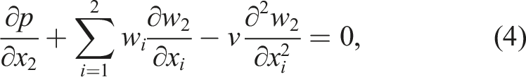
These assumptions naturally lead to the steady-state incompressible Navier-Stokes equations:

$\begin{array}{ll}\hfill -\nu \cdot \mathrm{\Delta }\mathit{w}(\mathit{x})+\left(\mathit{w}(\mathit{x})\cdot \nabla \right)\mathit{w}(\mathit{x})+\nabla p(\mathit{x})& =0\hfill \end{array}$

(1)

$\begin{array}{rr}\hfill \nabla \cdot \mathit{w}(\mathit{x})& =0,\hfill \end{array}$

(2)

where w ( x ) is an airflow velocity field and $p(\mathit{x})\in \mathbb{R}$ the pressure at a location x in the exploration domain $\mathrm{\Omega }\subset {\mathbb{R}}^2$ . Equation (1) is called momentum equation. The first term −ν ⋅ Δ w ( x ) describes a diffusion-like propagation of the velocity field. The parameter ν is the kinematic viscosity (Houghton et al., 2017). For our experiments, we assume air at 20°C and set ν = 1.510⁻⁵ m²/s (Foken, 2008). The second term $\left(\mathit{w}(\mathit{x})\cdot \nabla \right)\mathit{w}(\mathit{x})$ is an advective or convective acceleration (Song, 2018). The latter occurs when a fluid particle is transported by advection to a region with higher or lower velocity. In addition, the term ∇p( x ) represents the pressure gradient. Equation (2) is the continuity equation that means that there is no divergence of velocity in the fluid. In other words, there are no sources in the area. For the two dimensional case, we now have $\mathit{w}(\mathit{x})\triangleq {[w_1(\mathit{x}),w_2(\mathit{x})]}^{\mathrm{T}}\in {\mathbb{R}}^2$ , $\mathit{x}={[x_1,x_2]}^{\mathrm{T}}$ , and equations (1) and (2) become

$\frac{\partial p}{\partial x_1}+\sum _{i=1}^2{w}_i\frac{\partial w_1}{\partial x_i}-\nu \frac{{\partial }^2{w}_1}{\partial x_i^2}=0,$

(3)

$\frac{\partial p}{\partial x_2}+\sum _{i=1}^2{w}_i\frac{\partial w_2}{\partial x_i}-\nu \frac{{\partial }^2{w}_2}{\partial x_i^2}=0,$

(4)

$\frac{\partial w_1}{\partial x_1}+\frac{\partial w_2}{\partial x_2}=0,$

(5)

where we dropped the explicit dependency of w₁( x ) and w₂( x ) on the location x to simplify notation.

2.2. Boundary conditions

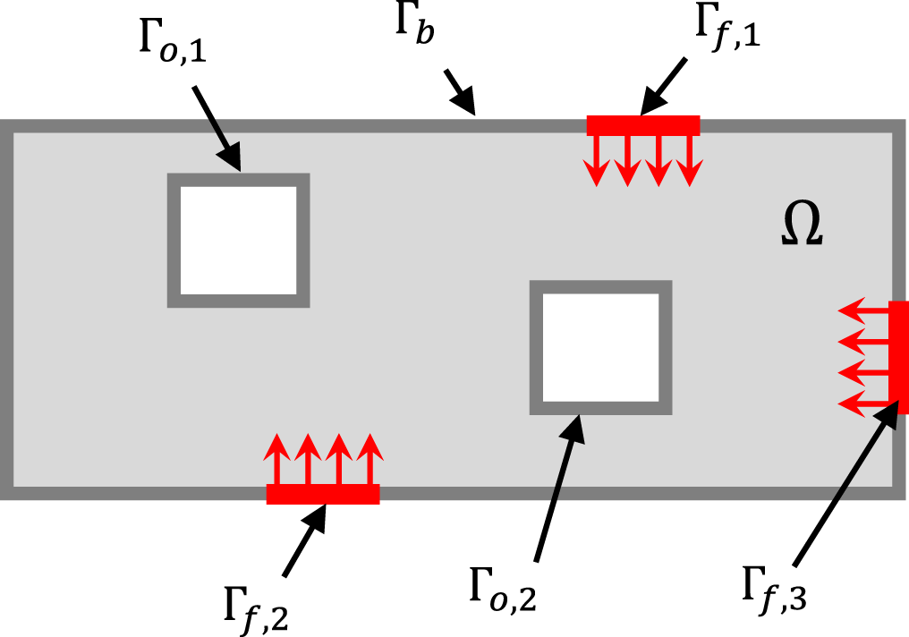
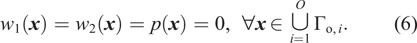
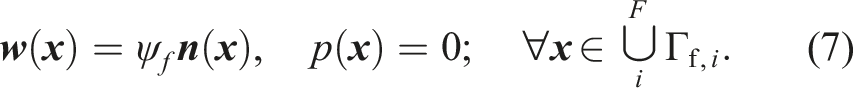
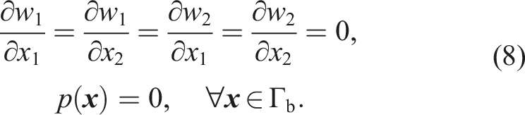
For a well-posed (unambiguous) description of the airflow field, the Navier-Stokes equations need to be extended by appropriate boundary conditions. In general, there are two different types of boundary conditions possible. On a Dirichlet bound, we define the actual value of a function (air velocity or pressure), whereas on a Neumann bound, the gradient of the function is specified. At this point, we would like to remark that throughout this article, we consider pressure as gauge pressure. So, zero pressure refers to ambient pressure. In our setup, three different boundaries of the domain Ω can be identified (see also Figure 1):

1. Obstacles (Dirichlet bound): In the exploration area, we consider O obstacles. The location of these obstacles is assumed to be known a priori. Furthermore, we assume that no air can flow across the boundaries of the obstacles. These are denoted by Γ_o,i (no-slip boundary condition); also we assume the pressure on the boundary to be zero. More formally,

$w_1(\mathit{x})=w_2(\mathit{x})=p(\mathit{x})=0,\forall \mathit{x}\in \bigcup _{i=1}^O{\mathrm{\Gamma }}_{\text{o},i}.$

(6)

• 2. Forced Inflow/Outflow (Dirichlet bound): We assume F regions of inflow on our boundary denoted by Γ_f,i, i = 1, …, F. In the experiments, we will implement this inflow by F fan-arrays on the outer bound of domain Ω. In these regions of the boundary, the air is blown into the domain in normal direction n ( x ) of the boundaries Γ_f,i with intensity ψ _f . Again, we assume the pressure p(x) to be zero at this boundary, that is,

$\mathit{w}(\mathit{x})={\psi }_f\mathit{n}(\mathit{x}),p(\mathit{x})=0;\forall \mathit{x}\in \bigcup _i^F{\mathrm{\Gamma }}_{\text{f},i}.$

(7)

• 3. Outer boundary (Neumann bound): The outer boundary Γ_b of Ω is assumed to be open so that the air can flow off the domain. Further, we assume that the conditions on the boundary regarding the airflow are constant with respect to the spatial location. This is modeled with a Neumann boundary condition for w ( x ) at Γ_b and a zero pressure assumption:

$\begin{array}{l}\hfill \frac{\partial w_1}{\partial x_1}=\frac{\partial w_1}{\partial x_2}=\frac{\partial w_2}{\partial x_1}=\frac{\partial w_2}{\partial x_2}=0,\\ \hfill p(\mathit{x})=0,\forall \mathit{x}\in {\mathrm{\Gamma }}_{\text{b}}.\end{array}$

(8)

As mentioned before, the airflow model is used in three different contexts: (i) for simulating the airflow in synthetic experiments, (ii) for the reconstruction of the airflow, and (iii) for the design of the exploration strategy. In the first context, equations (3)–(5) together with the three boundary conditions, result in a well-posed (forward) PDE problem. Solving this problem results in a well-defined, simulated airflow field.

Figure 1.

Different boundaries of the domain Ω used in experiments and simulations: Bounds Γ_o,i belong to obstacles, bounds Γ_f,i to inflow caused by fans, and Γ_b covers the remaining outer boundary.

In the second and third contexts, not all boundary conditions can be assumed as known; the airflow field, in this case, cannot be uniquely computed as the resulting problem is no longer well-posed. This leads to the problem of airflow exploration—an inverse problem of determining w ( x ) and p( x ) based on airflow measurements collected by the robots (see Section 3). For our purposes, in what follows, we will only assume known boundary conditions at obstacles, as the map of the environment is presumed to be available.

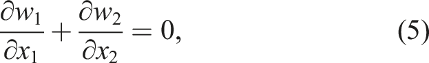
Let us also note that even though the airflow model is inspired by physics, it is merely an approximation of reality. In fact, there are a few effects that do lead to model mismatches due to the assumptions made. First, airflow is a 3D phenomenon. For instance, close to wall heaters in the lab, we would expect a vertical airflow component, violating the assumed 2D model and divergence-free assumption, that is equation (5). Furthermore, the assumption about the time-invariance of the airflow is a simplification; it is natural to expect time variability due to a number of factors, such as people’s movement in the lab and opening/closing doors. Nonetheless, our empirical evidence shows that the resulting model captures the global structure of the airflow while still having a manageable real-time computational complexity.

2.3. Nonlinearity of the model

A closer inspection of equations (3)–(5) reveals that they are nonlinear: the convection term $\left(\mathit{w}(\mathit{x})\cdot \nabla \right)\mathit{w}(\mathit{x})$ is bi-linear. A common approach to deal with the nonlinearity of Navier-Stokes equations is the Picard method (Rehman et al., 2008). It is a fixed-point iteration method with shown stability and global convergence (Pollock et al., 2019). In a nutshell, the idea of the method is the following. Instead of solving (3)–(5) at once, the solution is obtained iteratively. In particular, in each iteration k, the velocity w ^[k−1] from the previous iteration k − 1 is plugged into the nonlinear convection term. Specifically, equations (3) and (4) are modified as

$\frac{\partial p^{[k]}}{\partial x_1}+\sum _{i=1}^2{w}_i^{[k-1]}\cdot \frac{\partial w_1^{[k]}}{\partial x_i}-\nu \frac{{\partial }^2{w}_1^{[k]}}{\partial x_i^2}=0$

(9)

$\frac{\partial p^{[k]}}{\partial x_2}+\sum _{i=1}^2{w}_i^{[k-1]}\cdot \frac{\partial w_2^{[k]}}{\partial x_i}-\nu \frac{{\partial }^2{w}_2^{[k]}}{\partial x_i^2}=0,$

(10)

where superscript [k] indicates the iteration index; this linearizes the equations.

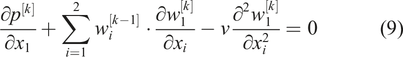
Now, considering w ^[k−1] as known, equations (9) and (10) together with equation (5) can be solved for w ^[k] at the iteration k. Then, the estimation is repeated for the next iterations. Starting from an initial guess w ^[−1] of the airflow field ¹ the Picard method convergences to the airflow ${\mathit{w}}^{*}=\underset{k\to \infty }{\lim }{\mathit{w}}^{[k]}$ that solves the nonlinear Navier-Stokes equations subject to our boundary conditions. Of course, in a numerical implementation letting k → ∞ is infeasible. We thus interrupt the iterations after some predefined number of steps. We will comment more on this aspect later in Section 3, when we discuss the airflow reconstruction results.

2.4. Numerical approximation

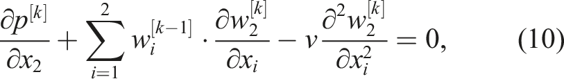
In order to solve the system of linear PDEs consisting of equations (5), (9), and (10), numerical approximation techniques are used. In our work, we use the Finite Element Method (FEM) for this purpose. FEM is a general numerical method for solving partial differential equations. In what follows, we provide a short overview of the approach applied to our problem. However, it is out of the scope of this article to explain FEM in full detail. For more information and details on FEM an interested reader is referred to textbooks like Zienkiewicz et al. (2013), Rehman et al. (2008), or Song (2018). In this article, it is only important to understand that FEM converts a variational PDE problem into a system of linear algebraic equations. In the following, we summarize some of the FEM key steps applied to the considered PDEs.

The FEM-based solution is obtained by first representing the PDE in a so-called weak formulation, which leads to a solution with respect to certain test functions. The exploration domain Ω is then discretized with a mesh of finite elements spanned over nodes. Based on the mesh, a finite set of basis (shape) functions ϕ _i , i = 1, …, N is defined to approximate continuous spatial functions. For example, the continuous airflow velocity component w₁( x ) in x₁ direction can be approximated as a weighted sum of N basis functions with the weights u _i (see also Figure 2): $w_1(\mathit{x})\approx {\sum }_i^N{u}_i{\varphi }_i(\mathit{x})$ . The same can be done for w₂( x ) and p( x ), as well as the test functions in the weak formulation; this approach is commonly referred to as the Galerkin method (Zienkiewicz et al., 2013).

Figure 2.

The spatial airflow field can be described by its velocity components w₁(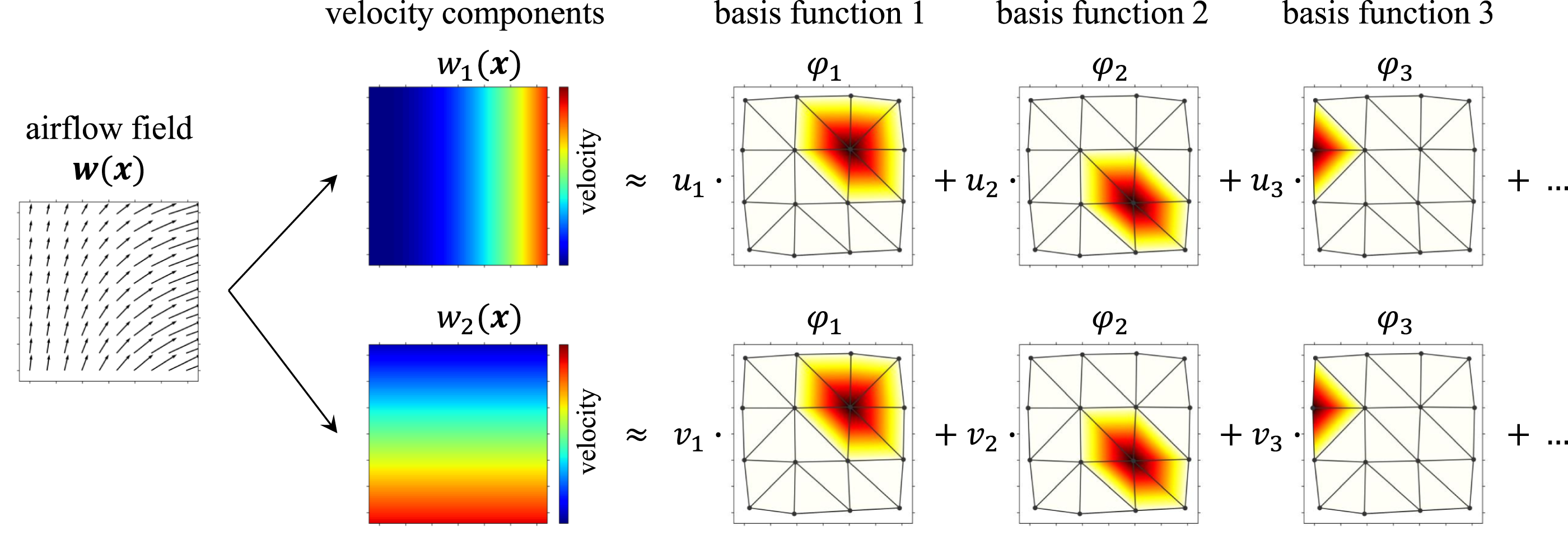 x ) and w₂( x ) in x₁ and x₂ direction. For the FEM approach, these continuous functions are approximated by a weighted sum of basis functions, where vector u and v aggregate the weights u₁… and v₁…. A basis function ϕ _i is only non-zero on those elements (triangles) of the mesh that contain the mesh node i. Note: Here, linear basis functions are depicted to illustrate the concept, whereas in the implementation second-order basis functions are used.

In our case, the wind field components w₁( x ) and w₂( x ) are represented with superposed quadratic basis functions on each element (second-order Lagrange element), and the pressure p( x ) by linear basis functions (first-order Lagrange element). ² The latter are fully parameterized by their values at the nodes of the mesh, that is, triangle vertices. For the former, an additional node is introduced in the middle of each edge of the mesh to account for an additional degree of freedom. By design, the basis functions are 1 at one particular mesh node and zero at every other node in the mesh. So the number N of the basis function and their weights are equal to the number of nodes in the mesh. Further, by this design, the weight u _i of a basis function is also equal to the approximated function value at the particular node. Note that for other points in space, the function of interest can be evaluated as a linear combination of the basis functions. The weights u _i used for representing function w₁( x ) are now collected in the vector u ; correspondingly, weights for the function w₂( x ) are collected in a vector v and for the pressure p( x ) in a vector p .

By inserting the discretized representations of all functions into the weak formulation of the linearized PDEs (9), (10), and (5), we arrive at a system of algebraic linear equations

$\begin{array}{l}\hfill {\mathit{L}}_1({\mathit{u}}^{[k-1]},{\mathit{v}}^{[k-1]})\left[\begin{array}{c}\hfill {\mathit{u}}^{[k]}\hfill \\ \hfill {\mathit{v}}^{[k]}\hfill \\ \hfill {\mathit{p}}^{[k]}\hfill \end{array}\right]=\mathbf{0},\end{array}$

(11)

$\begin{array}{l}\hfill {\mathit{L}}_2({\mathit{u}}^{[k-1]},{\mathit{v}}^{[k-1]})\left[\begin{array}{c}\hfill {\mathit{u}}^{[k]}\hfill \\ \hfill {\mathit{v}}^{[k]}\hfill \\ \hfill {\mathit{p}}^{[k]}\hfill \end{array}\right]=\mathbf{0},\end{array}$

$\begin{array}{l}\hfill {\mathit{L}}_3\left[\begin{array}{c}\hfill {\mathit{u}}^{[k]}\hfill \\ \hfill {\mathit{v}}^{[k]}\hfill \end{array}\right]=\mathbf{0}.\end{array}$

where L ₁( u ^k−1, v ^k−1) and L ₂( u ^k−1, v ^k−1) are matrices obtained by discretizing (5), (9), and (10), respectively. Note that L ₁ and L ₂ depend on the values of the parameters at iteration k − 1 due to the Picard approximation method (see Section 2.3). We skip the details of obtaining (11) as they are rather straightforward and again refer the reader to Zienkiewicz et al. (2013) for more detail.

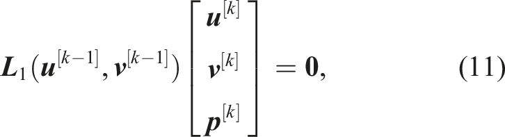
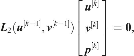
As the final step, we extend (11) with the discretized versions of the boundary conditions. For Dirichlet boundaries, we then obtain:

${\mathit{B}}_u{\mathit{u}}^{[k]}={\mathit{b}}_u,{\mathit{B}}_v{\mathit{v}}^{[k]}={\mathit{b}}_v,{\mathit{B}}_p{\mathit{p}}^{[k]}=\mathbf{0}$

(12)

where the matrices B _u , B _v , and B _p are selection matrices that pick entries of the corresponding vector u , v , and p belonging to mesh nodes on the respective boundaries. The vectors b _u and b _v then contain values at the boundaries corresponding to its type: zeros for obstacles and non-zero values at nodes corresponding to fan locations. The homogeneous Neumann boundary condition is naturally included in the weak formulation of our PDE (see Zienkiewicz et al. (2013)); thus, there is no need for a separate equation to take it into account.

Obviously, when some of the boundary conditions are unknown, as it is in the case of airflow exploration, the corresponding structure of the matrices L ₁, L ₂, L ₃, as well as B _u , B _v , and B _p have to be modified to exclude information about unknown nodes. Again, this is a standard step within FEM approach, and we skip the details for brevity.

Now, to simplify further notation, we define the parameter vector θ ≜ [ u , v , p ] that collects all unknown parameters. This allows us to write (11) more compactly as

$\mathit{L}({\mathit{\theta }}^{[k-1]}){\mathit{\theta }}^{[k]}=\mathbf{0}.$

(13)

Similarly, the boundary conditions (12) can be then represented as

$\mathit{B}{\mathit{\theta }}^{[k]}=\mathit{b}.$

(14)

Again we would like to mention that if sufficient boundary conditions are known, equations (13) and (14) are well-posed and solvable. This allows us to simulate an artificial airflow field. However, in the case of the exploration task, not all boundary conditions are known, for example, inflow and outflow. In this case, the equations are ill-posed, and additional measurements are required to estimate the airflow field.

3. Map reconstruction

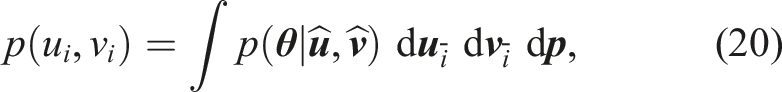
The main objective of the exploration task is to obtain a map of the airflow field. In other words, for every point in the domain Ω we want to know the x₁ and x₂ components of the airflow velocity. Therefore, spatially distributed measurements of the airflow are needed. Based on our airflow model introduced in the previous sections, we are able to interpolate in a physics-informed way between rather sparse sampling points. Basically, the map reconstruction reduces to estimating the parameters of the airflow model, that is, the vectors u and v . ³ To this end, we use a Bayesian MAP approach, which we construct as explained in the following.

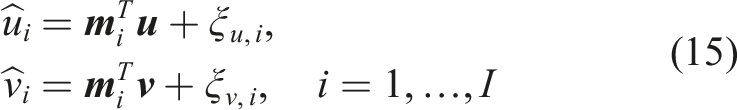
The robots are equipped with anemometers to measure the airflow components at their current position. The I measurements can be modeled mathematically as

$\begin{array}{ll}\hfill {\widehat{u}}_i& ={\mathit{m}}_i^T\mathit{u}+{\xi }_{u,i},\hfill \\ \hfill {\widehat{v}}_i& ={\mathit{m}}_i^T\mathit{v}+{\xi }_{v,i},i=1,\dots ,I\hfill \end{array}$

(15)

where m _i is a vector with zeros except for the location that corresponds to the mesh node at which the robots take the measurement. These elements are 1. It thus selects an appropriate element from vector u and v that belongs to the position of the robot. In our approach, we only consider the mesh nodes as possible locations for measurements. However, also measurements in between could be considered by modifying m as an interpolation operator, for example, with a weighted summation of nearby node values. We assume that the measurements are corrupted by independent additive Gaussian noises ξ_u,i and ξ_v,i with zero mean and variance σ² = 1/τ _m . This Gaussian assumption is well supported by the collected empirical evidence. In Figure 3, we show a fit of a Gaussian Probability Density Function (PDF) to histograms of the recorded airflow measurements in our experimental setup. As we see, the approximation is well justified.

Figure 3.

The plots depict histograms of measured data for the airflow velocity components u and v at a single representative location in our experimental area. The data set covers 20 minutes. In addition, a fitted Gaussian distribution is plotted.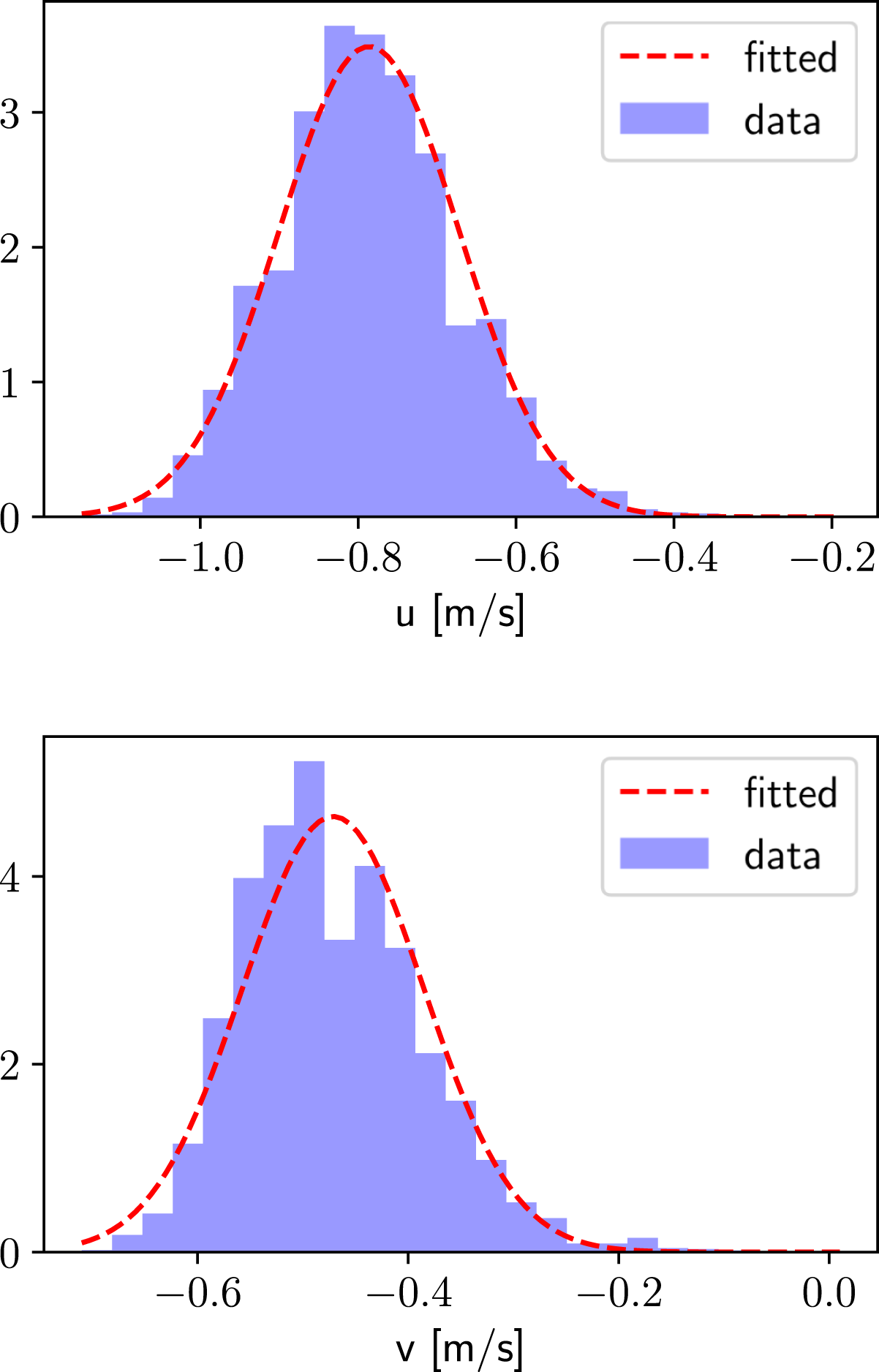

Now, using (15) we can formulate the likelihood of the airflow parameters θ as

$p\left(\widehat{\mathit{u}},\widehat{\mathit{v}}|\mathit{\theta }\right)\propto e^{-{\tau }_m/2 \Vert {\mathit{M}}_u\mathit{\theta }-\widehat{\mathit{u}}{\Vert }^2-{\tau }_m/2 \Vert {\mathit{M}}_v\mathit{\theta }-\widehat{\mathit{v}}{\Vert }^2},$

(16)

where $\widehat{\mathit{u}}\triangleq {[{\widehat{u}}_1,\dots ,{\widehat{u}}_I]}^T$ , $\widehat{\mathit{v}}\triangleq {[{\widehat{v}}_1,\dots ,{\widehat{v}}_I]}^T$ , and M _u and M _v are the selection matrices constructed of vectors m ₁, …, m _I for u- and v-components of the airflow, respectively.

The Bayesian approach allows us to encode a priori knowledge in the form of a prior PDF. Here, the airflow model is used for this purpose. In the first step, we cast the deterministic model given by (13) and (14) into a probabilistic framework. We do this by relaxing (13) and allowing the equality to deviate from 0. Specifically, we assume that L ( θ ^[k−1]) θ ^[k] = r where r is a residual with the property that it follows a white Gaussian distribution with zero mean and precision τ _s . In a similar fashion, we relax (14): We treat the difference ( Bθ ^[k] − b ) to be random, following a white Gaussian distribution with zero mean and a precision parameter τ _b .

We note that such a modeling approach has been previously introduced by Wiedemann et al., (2019a), however, for a different type of PDE. Now, we can design a prior PDF for θ as follows:

$p(\mathit{\theta })\propto e^{-\frac{{\tau }_s}{2}\Vert \mathit{L}\mathit{\theta }{\Vert }^2}{e}^{-\frac{{\tau }_b}{2}\Vert \mathit{B}\mathit{\theta }-\mathit{b}{\Vert }^2}{e}^{-\frac{{\tau }_p}{2}\Vert \mathit{\theta }{\Vert }^2}.$

(17)

Here, we dropped the iteration counter k for simplification, but we will comment on it later on. The first two factors account for the discretized PDE model and the boundary conditions, respectively. The third factor $e^{-{\tau }_p/2\Vert \mathit{\theta }{\Vert }^2}$ in (17) is an additional regularization term. Its role is to stabilize (or smooth, to be more precise) the maximization of the posterior function, especially in the early phases of the exploration when there are only a few measurements available.

Thus, the selected prior, on the one hand, favors parameter choices θ that fulfill the Navier-Stokes equations; on the other hand, we favor airflow fields with low velocities and make the problem well-posed.

Finally, from the Bayes theorem, we formulate the posterior PDF of the parameters θ as

$p(\mathit{\theta }|\widehat{\mathit{u}},\widehat{\mathit{v}})\propto p(\widehat{\mathit{u}},\widehat{\mathit{v}}|\mathit{\theta })p(\mathit{\theta }).$

(18)

The MAP estimate of the airflow parameters u and v can then be obtained by maximizing the posterior function:

$\underset{\mathit{u},\mathit{v},\mathit{p}}{\mathrm{a}\mathrm{r}\mathrm{g}\mathrm{m}\mathrm{a}\mathrm{x}} p\left(\mathit{\theta }|\widehat{\mathit{u}},\widehat{\mathit{v}}\right),$

(19)

where u , v are actually hidden in θ . It can be shown that, in the log domain, the optimization transforms into a standard regularized least squares problem. This occurs because the right-hand side of (19) follows a Gaussian distribution and, thanks to the Picard method, is quadratic in θ . At this point, it is essential to highlight that (19) essentially resolves our inverse problem by finding u , v and p that best align with the observations $\widehat{\mathit{u}},\widehat{\mathit{v}}$ and matches the model assumptions in the least squares sense. It is crucial to underscore that, without measurements and regularization, this optimization problem would be ill-posed. The model assumptions grounded in the Navier-Stokes equation already narrow down the solution space. However, this is not enough to render the problem (19) well-posed. Due to the presence of unknown boundary conditions, the solution to (19) lacks uniqueness without the incorporation of measurements and regularization.

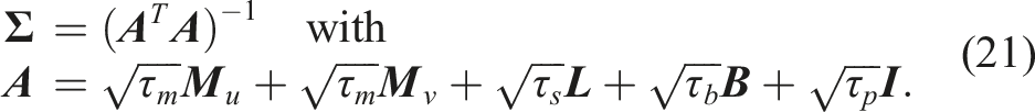
Let us make a few remarks about the choice of precision parameters τ _m , τ _s , τ _b , and τ _p . These parameters weight the corresponding contributions in the posterior (18) from the measurement likelihood, the model and boundary equations, and the regularization term, respectively. While τ _m is related to the amount of measurement noise, the other parameters encode our “trust” in the other model assumptions. For example, increasing τ _s puts more emphasis on the fulfillment of the Navier-Stokes equation. Decreasing τ _b allows the solution to deviate from assumed boundary conditions. The parameter τ _p regularizes the posterior and, in general, should be selected as low as possible while still ensuring the numerical stability of the problem. Later in Section 6, we will provide numerical values for the selected parameters used in the simulations and experiments.

Due to the nonlinearity of the Navier-Stokes equations and the Picard method, map estimation is an iterative approach. For every iteration k the matrix L needs to be updated based on the previously estimated u ^[k−1] and v ^[k−1]. The update loop runs continuously in our implementation, and whenever new measurements are available, they are directly plugged into the likelihood equation (16).

4. Exploration strategy

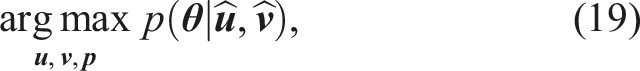
The previous section deals with the reconstruction of the airflow given spatially distributed measurements $\widehat{\mathit{u}}$ and $\widehat{\mathit{v}}$ . Here, we now address the procedure for collecting the measurement samples. Our objective is to develop a strategy that collects samples in an informative (active) manner; in other words, we would like to ensure that the collected samples are as informative as possible to accelerate the airflow reconstruction. Such approaches for collecting measurements are often referred to as active learning approaches (Taylor et al., 2021).

The proposed exploration approach is based on the uncertainty information contained in the posterior (18) (see also Wiedemann et al., 2019a). Precisely, we quantify the spatial uncertainty distribution based on (18). We consider a multi-robot system consisting of a fixed number of robots and send these robots to the locations in the exploration domain Ω where the uncertainty is high. When the robots have taken new measurements, we can update the uncertainty distribution and again send the robots to locations that have now become the most uncertain ones. These locations are good candidates for taking the next samples since a measurement at these locations would naturally reduce the uncertainty there, which in turn will bring down the overall uncertainty of the estimated airflow. Due to our used discretization, each parameter in θ is associated with a node in the spatial discretization mesh. So, by associating the uncertainty of each parameter with the corresponding mesh node location, we can compute a spatial uncertainty map. In our case, we are interested in computing the uncertainty of airflow parameters u _i and v _i for each node i in our discretization mesh.

As a measure of uncertainty, we look at the covariance of the posterior distribution of u _i and v _i obtained by marginalizing the posterior over all other nodes $\overline{i}$ :

$p(u_i,v_i)=\int p(\mathit{\theta }|\widehat{\mathit{u}},\widehat{\mathit{v}})\mathrm{d}{\mathit{u}}_{\overline{i}}\mathrm{d}{\mathit{v}}_{\overline{i}}\mathrm{d}\mathit{p},$

(20)

where ${\mathit{u}}_{\overline{i}}$ and ${\mathit{v}}_{\overline{i}}$ are vectors u and v with the ith node excluded. Since the posterior is a Gaussian, computing its posterior covariance Σ is rather straightforward. It can be shown that

$\begin{array}{ll}\hfill \mathbf{\Sigma }& ={({\mathit{A}}^T\mathit{A})}^{-1}\text{with}\hfill \\ \hfill \mathit{A}& =\sqrt{{\tau }_m}{\mathit{M}}_u+\sqrt{{\tau }_m}{\mathit{M}}_v+\sqrt{{\tau }_s}\mathit{L}+\sqrt{{\tau }_b}\mathit{B}+\sqrt{{\tau }_p}\mathit{I}.\hfill \end{array}$

(21)

Now, the marginal posterior covariance Λ _i of the node i can be extracted from Σ as

${\mathbf{\Lambda }}_i=\left[\begin{array}{cc}\hfill {\mathbf{\Sigma }}_{j,j}\hfill & \hfill {\mathbf{\Sigma }}_{j,k}\hfill \\ \hfill {\mathbf{\Sigma }}_{k,j}\hfill & \hfill {\mathbf{\Sigma }}_{k,k}\hfill \end{array}\right],$

(22)

where k is the index in θ that corresponds to the element u _i , and j is the index corresponding to v _i , respectively. For our two-dimensional airflow field, we obtain the 2 × 2 matrix Λ _i .

There are different possibilities to quantify the resulting uncertainty of the node i. Here, we use the trace tr(Λ _i ), which is related to a so-called A-optimality criterion in optimal experimental design (Pukelsheim, 1993). This can be interpreted as an averaged variance of the estimated wind directions per node. A high variance (or a high trace) would thus correspond to a high uncertainty of the node. This measure needs to be computed for each node i in the mesh representation. In general, other criteria could be considered to extract a scalar uncertainty metric from the covariance matrix at each node, such as the determinant of the matrix, that is, D-optimality in optimal experimental design. By linearly interpolating the computed uncertainties between the nodes, we obtain the desired spatial uncertainty map. An example of such a map is shown in Figure 15(c). This map is then used for actual path planning and coordination of the robots, as will be explained in the following.

5. Multi-robot system

In this section, we describe the proposed airflow exploration approach from a system-level perspective and discuss some implementation aspects of both software and hardware used in experiments.

5.1. Exploration procedure

To collect the measurements for airflow exploration, we use a swarm of robots. We assume that the robots have the following key capabilities:

Localization: The robots should be able to localize themselves with respect to the environment.

Sensing: Each robot should be able to measure the u- and v-components of the airflow at their current location

Intelligence: The robots should have on-board computing resources to compute an informative location for the next measurement

Navigation: The robots should be able to plan and execute a path toward the next location without colliding with obstacles or other robots

The flow chart of the system making use of these capabilities is shown in Figure 4. Each robot has its own instance of the sensor unit (anemometer), motor controller, and path planner. In the first step, each robot measures the airflow vector with an onboard anemometer. The measurements are averaged over 10 s to smooth out short-term turbulence effects. During this period, the robot stands still. The average measurement, together with the robot’s current location, is sent to the model update block, where the reconstruction takes place. The model parameters are continuously updated, resulting in the computed airflow and uncertainty map as detailed in Section 3 and Section 4. The results of these computations are stored in a database which can then be accessed by the robots or system operators.

Figure 4.

The flow chart illustrates the system architecture of the implemented exploration strategy. Dashed lines indicate information flow and solid lines show the process flow. Blue boxes represent actions supported by software modules, as shown in green.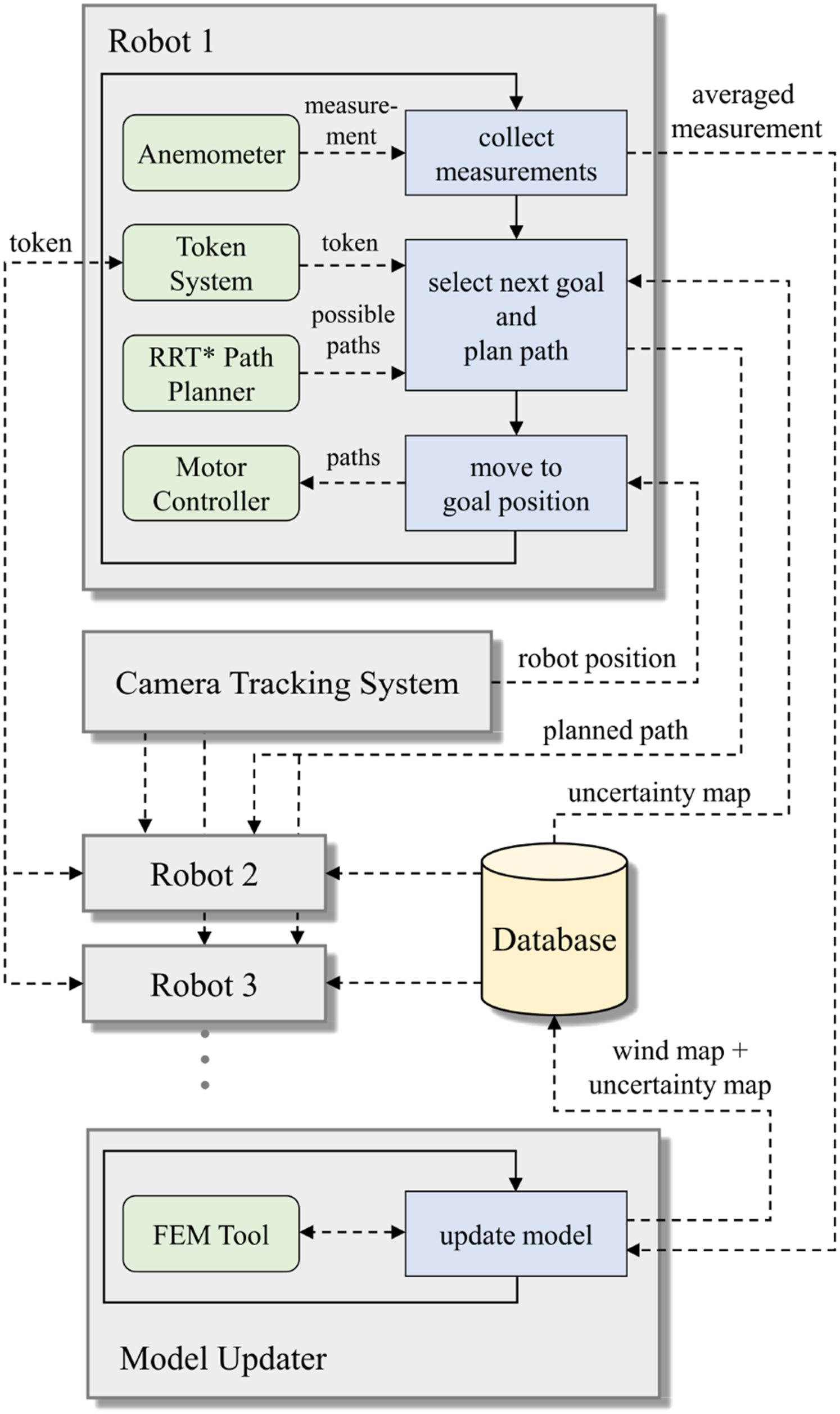

After taking one measurement, a robot then selects a new location for the subsequent measurement and plans a collision-free trajectory toward it. To this end, it requests the most recent estimate of the uncertainty map from the database shared by the swarm. Selection of a particular point and path planning toward it is secured by a token system to ensure the unique assignment of the measurement location to a robot (see also Section 5.3). To compute trajectories toward selected measurement locations that are safe and collision-free a modified version of an RRT* algorithm is used (LaValle, 1998). We will discuss the RRT* planner in Section 5.2 in more detail. The output of the algorithm is a set of possible collision-free trajectories from which the path leading to the highest uncertainty at the destination is chosen.

The selected trajectory is then handed over to the motor controller that drives the motors of the robot and ensures the robot follows the calculated path. When the robot reaches the endpoint of the path, the whole cycle repeats anew. In our approach, the robots only need to communicate concerning the token system and exchange information about the planned path with each other (see Figure 4).

Let us emphasize that the exploration cycles of individual robots run completely asynchronously. As a result, the time it takes robots to complete their exploration cycle will differ as each robot has different traveling times.

5.2. Path planner

A path planner is needed to compute a safe trajectory toward the new measurement position avoiding both static and dynamic obstacles. We implement the planner using a Rapidly-Exploring Random Tree (RRT)* algorithm (Karaman and Frazzoli, 2011; LaValle, 1998). The algorithm generates multiple possible paths in the allowed free space of the exploration area and takes into account robot dynamic constraints. For our experiments, we generate paths consisting of straight segments, which can be easily followed by our differential-drive, tracked robots.

To ensure the avoidance of other moving robots, the swarm exchanges the planned paths. To make sure that no collision can occur, a robot is not allowed to cross the already planned trajectories of other robots. Additionally, a safety margin around the trajectories is defined to compensate for the robot’s exterior dimension and inaccuracies in the localization system. Similarly, we define a safety margin around static obstacles, which we set to 0.5 m in our experiments. In Figure 5, we show an example of generated possible trajectories, marked in green, for a robot located at (−1, −4). These possible trajectories exemplify the generated RRT* tree used for navigation toward a new measurement position. The trajectories of three other robots are shown in red. The dotted lines mark the safety margin around these trajectories. The static obstacles are shown in blue.

Figure 5.

This plot shows an example situation with two obstacles and four robots. All possible paths planned by the RRT* Path Planner are shown in green for the robot located at (−1, −4). Dots indicate the locations where the robot changes its orientation. The obstacles and paths of other robots are extended by a safety margin. They are blocked areas for the path planner.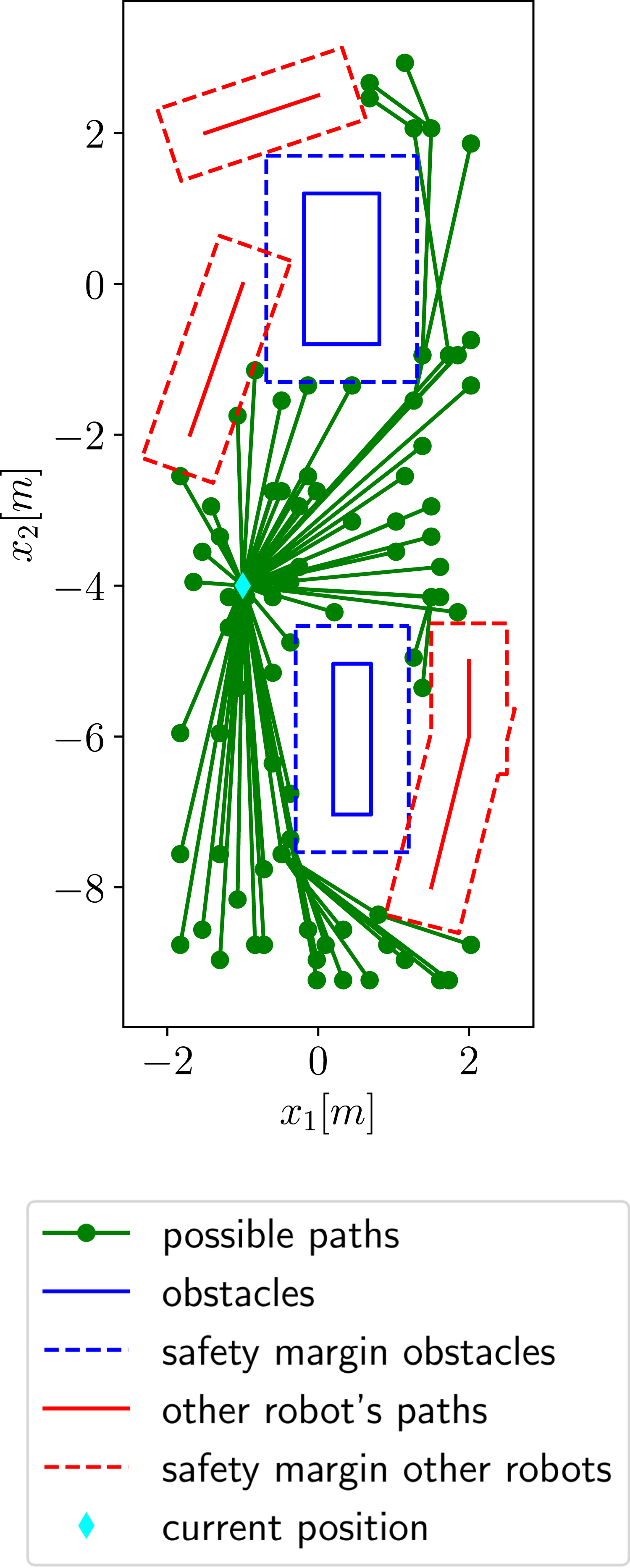

In real-world experiments, we observed that due to inaccuracy in the positioning system, a robot might stop closer to either an obstacle or another robot, slightly violating the safety margin. While this is not critical from a safety perspective, it might cause issues when the robot plans its next path since RRT* would return no possible trajectories due to the origin of the tree being inside the safety margin. As a workaround, we use the following fallback routine: if the RRT* root lies within the safety margin, it is “moved” into the free space by determining the distance and direction to the closest obstacle border. The RRT* starting point is then shifted accordingly into the free space with an additional tolerance (5 cm in our case). Then, the tree is generated as usual.

After the RRT* tree has been generated, the uncertainty map is taken into account to choose from all nodes of the tree (intermediate nodes and end nodes) the node with the highest uncertainty as the next measurement location. The path to this node from the robot’s current position is found by “backtracking” the tree nodes. To follow the created path, a list of nodes belonging to the path is sent to the motor controller, which translates the straight lines into commands for the motors.

5.3. Token system

Due to the asynchronous distributed functioning of the system, it is essential to ensure that two robots do not plan a path at the same time, as this might cause collisions of the trajectories or result in the selection of the same measurement location. As the system runs in a distributed fashion without a centralized controller, we need a token system that prevents such situations. It is important to emphasize that only the planning step is forbidden to be executed in parallel. However, as soon as the planning is completed, robots can execute the collision-free paths simultaneously and in parallel.

Initially, one of the robots holds the token for as long as no one else requests it. The token holder continuously broadcasts its own ID/name to all robots, indicating the current token holder. We also use this information to detect possible timeouts of the token holder and reinitialize the token system in case of a failure. Then, a robot that wants to plan a new trajectory requests the token and broadcasts its request. The role of the token holder is to collect requests in a FIFO list and, as soon as it is done with its own path planning (which typically took about 1 sec in our experiments), pass the list with a token to the robot on top of the list. The receiving robot then becomes the new token holder. The list of robots that currently request the token is also continuously sent out by the token holder. This is needed by other robots in case of a timeout due to failures of the current token holder to determine the next token holder.

5.4. Robotic platform

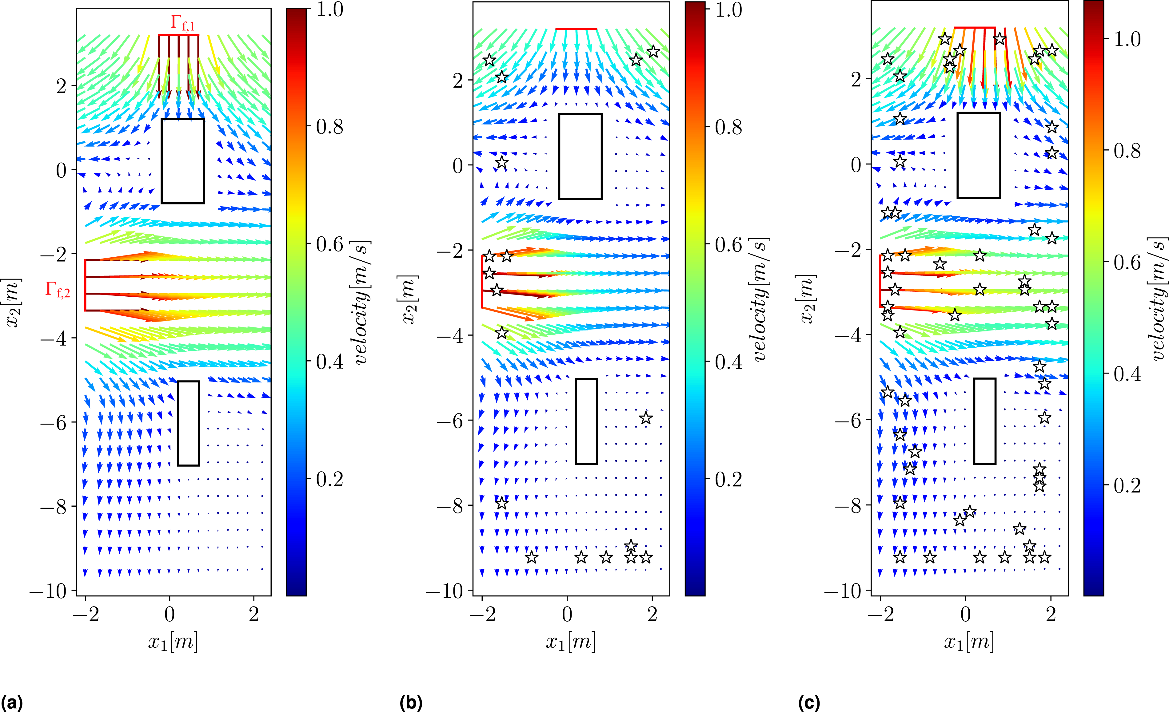
In the experiments, we use non-holonomic rovers (see Figure 6). Two tracks allow the robot to turn and move forward and backward. Each robot is equipped with a TriSonica Mini anemometer (Anemoment.com, nd). It is an ultrasonic anemometer that measures wind speeds in all three spatial directions in a range from 0–50 m/s with an accuracy of ±0.2 m/s and a resolution of 0.01 m/s. Note that for the experiments, we only consider the horizontal wind components for the u- and v-directions. The wind measurements are taken at a rate of 5 Hz.

Figure 6.

CAD design of the rover used in our experiments equipped with anemometer.

Figure 7.

Quiver plots of example airflow fields: Panel (a) shows a simulated airflow field obtained through simulation. In (b), the estimated airflow field is shown after 2 min of exploration, and in (c) after 10 min. The white stars indicate the locations where measurements were taken.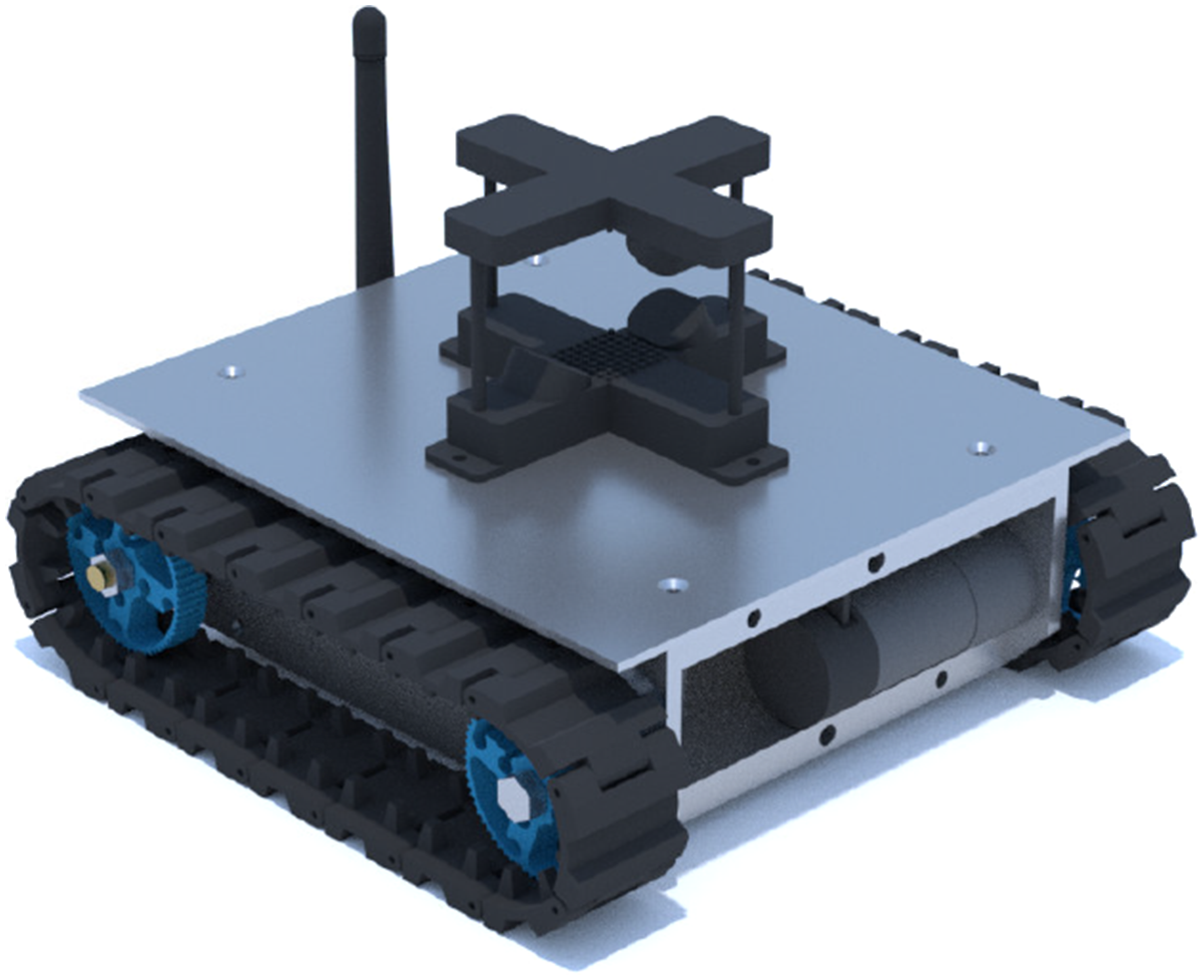

The robots carry a Raspberry Pi 4 onboard computer. This computer is responsible for receiving the measurements from the anemometer, communicating with the motor drivers, as well as, low-level path tracking.

All of the experiments are conducted in a laboratory equipped with a camera tracking system providing the position and orientation of all robots with centimeter accuracy in real-time. This information is used by the low-level path planner to follow the planned trajectories and to label measurements with a precise location. Further, during exploration, the orientation of the robots is used to transform the wind measurements into a common global coordinate system (i.e., u and v components).

The robots are also equipped with a commercial WiFi communication system. This allows the robots to (i) receive their current position and orientation from the tracking system, (ii) send measurements to the central model update software module, (iii) access the database, and (iv) safely plan paths secured by the token systems (as detailed in Figure 4). The whole software is implemented based on the Robot Operating System 2 (ROS2). This publisher-subscriber framework facilitates inter-process communication over the network.

6. Evaluation

In the following section, we evaluate the proposed approach in simulations as well as in lab experiments. Since we intend to accurately map the airflow field, a desirable performance criterion would be an error between an estimated and an actual ground truth airflow. Unfortunately, it is hard to quantify this error in real-world experiments—even in a controlled environment—since the ground truth airflow field is rarely known. Consequently, we evaluate our approach in two steps: First, we virtually simulate the airflow field and thus have full control over all environmental parameters, for example, boundary conditions. Further, the simulation provides us with ground truth information about the actual airflow that we can compare to the estimated airflow map and thus quantify the estimation error. Second, we use a swarm of robots in a controlled laboratory environment to experimentally validate the exploration approach. Here, we cannot precisely quantify the estimation error due to the lack of ground truth information. However, we can provide a proof-of-concept, investigate the convergence of the estimation, and compare the exploration strategy to other sampling approaches.

6.1. Simulation

6.1.1. First example

We consider an exploration domain of 4 m × 13 m to mimic the dimensions of the lab used in the experimental evaluation later on. We placed two inflow boundaries: Γ_f,1 at (x₁ = 0, x₂ = 3) and Γ_f,2 at (x₁ = −2, x₂ = −3) with w₂( x ) = −1; x ∈ Γ_f,1 and w₂( x ) = 1; x ∈ Γ_f,2. For the remaining outer bound Γ_b, we assume Neumann boundary conditions that allow the free exchange of air. Further, two obstacles Γ_o,1 and Γ_o,2 are placed in the environment with no-slip boundary condition w₁( x ) = 0; w₂( x ) = 0; x ∈ Γ_o,1⋃Γ_o,2. With these boundary conditions, the problem is well-posed, which allows us to solve the PDEs without any measurements and thus calculate the ground truth airflow field used for simulation. The result of this simulation is shown in Figure 7(a).

To estimate the airflow from the measurements, we use five robots that collect airflow samples and move according to the proposed exploration strategy. For the robots, the placement of the fans is unknown, so measurements are necessary to solve the now ill-posed problem. Whenever a robot has reached its goal position and wants to take a measurement, the measurement value is taken from the simulated ground truth airflow field at the robot’s current position.

The reconstructed solution for a single simulation run after 2 and 10 min of exploration is shown in Figures 7(b) and (c), respectively. White stars indicate the locations of the taken measurements. As can be seen from Figure 7(b) after 2 min, the robots primarily measure at border areas of the domain since they are most uncertain due to the lack of boundary conditions in the model. In Figure 7(b), measurements close to the inflow Γ_f,2 were already carried out, and in general, the estimate is quite close to the ground truth airflow field except for the region around the inflow Γ_f,1. After 10 min, it can be seen in Figure 7(c) that the ground truth was reconstructed quite accurately everywhere since enough measurements have been collected to estimate the airflow field correctly.

Figure 8.

NRMSE between the estimated airflow field and the ground truth over time: In (a) in red, the example corresponding to Figure 7 is shown together with the averaged error over 10 simulation runs in dotted blue. The area in blue indicates the maximum and minimum observed error in 10 simulation runs. In (b), the error curves for different setups of obstacles and inflow conditions are depicted (each averaged over 10 runs). The average is shown in black, and the maximum and minimum observed errors are indicated by the gray area.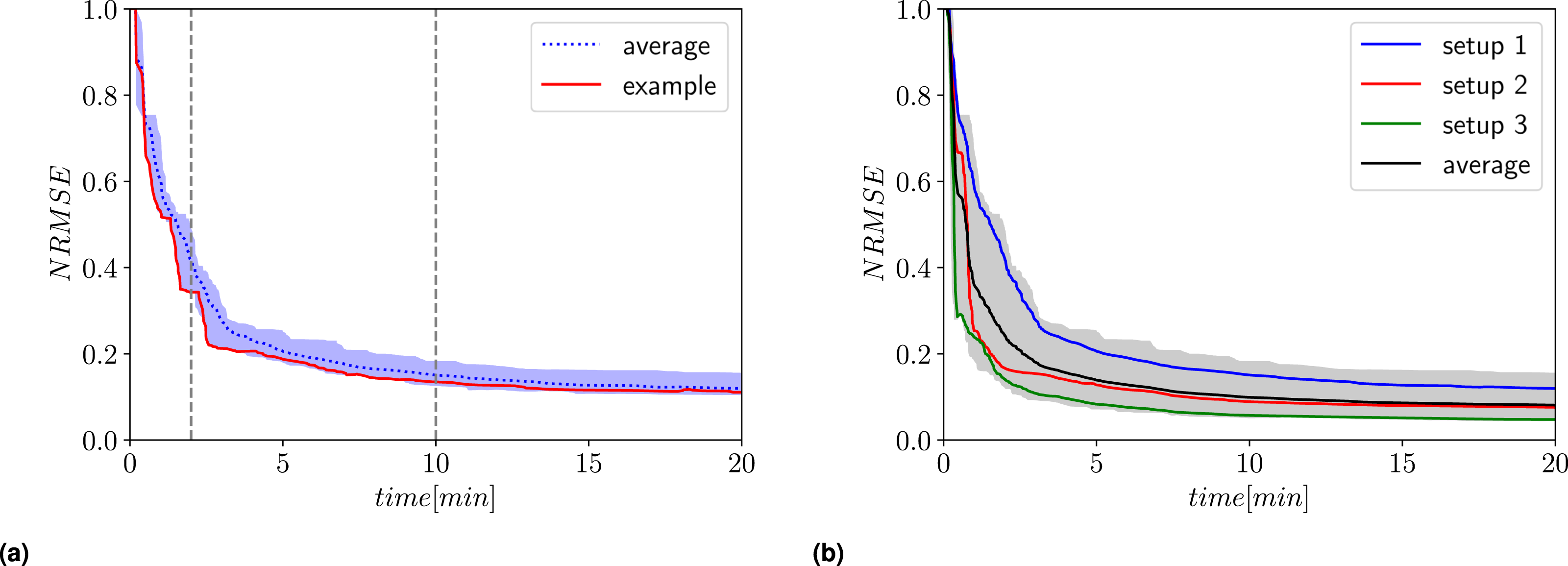

6.1.2. Performance evaluation

The model and the airflow map are updated iteratively as explained in Section 2 and Section 3. This update loop runs at a fixed rate. The simulation enables us to calculate for every update iteration k the NRMSE between the ground truth u _gt, v _gt and the current estimated airflow field u ^[k], v ^[k] computed as:

$e_{\mathit{NRMSE}}^k=\sqrt{\frac{\Vert {\mathit{u}}_{\text{gt}}-{\mathit{u}}^{[k]}{\Vert }^2+\Vert {\mathit{v}}_{\text{gt}}-{\mathit{v}}^{[k]}{\Vert }^2}{\Vert {\mathit{u}}_{\text{gt}}{\Vert }^2+\Vert {\mathit{v}}_{\text{gt}}{\Vert }^2}}.$

(23)

The corresponding results are shown in Figure 8(a), where the red curve corresponds to the sample run shown in Figure 7. In the beginning, the error decreases rapidly, but after approximately 5–10 minutes, it stagnates. This indicates that the area is already well-covered with measurements, and new measurements do not provide much new information to improve the estimate. This is a generally observed behavior in our simulations. In Figure 8(a), the mean and range between maximum and minimum errors for 10 simulation runs are depicted in blue, indicating the similarity of the behavior. In Figure 8(b), we also show the error curves for different setups where the locations of air fans were randomly varied. Each curve is averaged over 10 simulation runs (30 in total). For the different setups, the location of the inflow boundaries and obstacles varied. As can be seen, the performance slightly depends on the setup. So, setup 3 seems to be explored faster with a lower estimation error than setup 1, which we investigated in Figure 7. Nevertheless, in all cases, the proposed exploration strategy performs very well. However, we want to draw the reader’s attention to the fact that the error does not reach zero even though the measurements fit exactly the ground truth data and are not disturbed by noise. This effect can be explained by the model regularization term and particular choices of the other model parameters τ _m , τ _s , and τ _b . These were set to 1, while the regularization parameter τ _p was set to τ _p = 10⁻⁴. Regularization is necessary to make the problem well-posed when few data samples are available. Yet, at the same time, it biases the solution and prevents the error from reaching zero. We will have a closer look at the effect of these parameters later on in the evaluation of the experiments, where the measurement noise also plays a role.

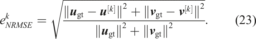
Unfortunately, the NRMSE is not an intuitive measure and is hard to interpret. To address this limitation, we present the error in the estimated airflow speed, that is, the amplitude of the airflow, in Figure 9(a), and the error in the estimated airflow direction in Figure 9(b). Both estimates correspond to the example depicted in Figure 7(c) after 10 minutes of exploration. The error is calculated as the difference between the ground truth airflow field and the estimated one. As observed, the error in the airflow velocity mostly remains below 0.1 m/s. Only in regions with high airflow and where the airflow encounters obstacles does the error slightly increase. Similarly, the error in direction predominantly stays below ±15deg. According to Wiedemann et al. (2019a), these errors are deemed small enough for robotic gas source localization, which is the primary motivation behind our work. In this context, one might also consider the specification of the sensor used in experiments to better interpret the performance of our approach. The used ultrasonic anemometer can measure the three spatial directions with an accuracy of ±0.2 m/s (Anemoment.com, nd). So the estimation error is already below the sensor accuracy.

Figure 9.

The plots depict the error in the estimated airflow field with respect to the airflow velocity amplitude in (a) and airflow direction in (b). In (b), areas with velocities below 0.1 m/s are masked since the direction of a vector loses its meaning when the vector’s amplitude approaches zero.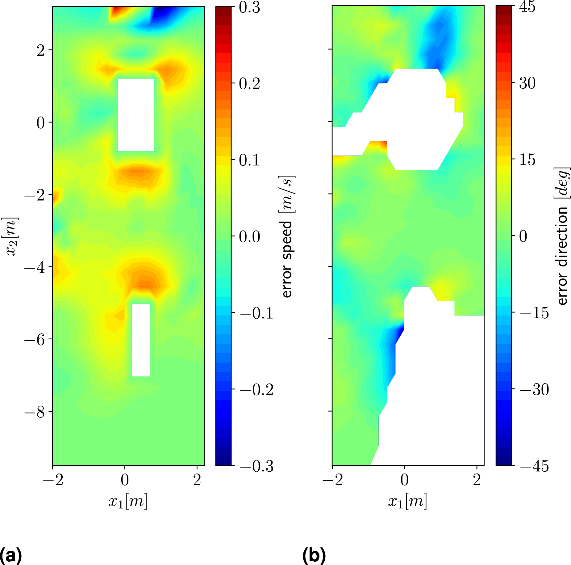

Figure 10 shows the number of taken measurements over time and the number of distinct measurement locations for three different evaluated setups. The curves show no horizontal slopes, which implies that robots continuously take measurements. The plot also shows that there are more measurements than distinct measurement locations. This means some locations are measured twice, which might be inefficient for exploration. This situation can occur in cases where a robot is forced to measure at an already visited location when no other locations are reachable because of other robots and obstacles blocking the path. In the early phase of the exploration, this is not very likely. However, with an increasing number of visited locations, the effect gets more significant. Nonetheless, according to Figure 8 the estimate of the airflow after 10 min is already sufficiently accurate. For this time duration, approximately 15% of measurement locations have been revisited.

Figure 10.

Number of measurements and the number of distinct measurement locations over exploration time.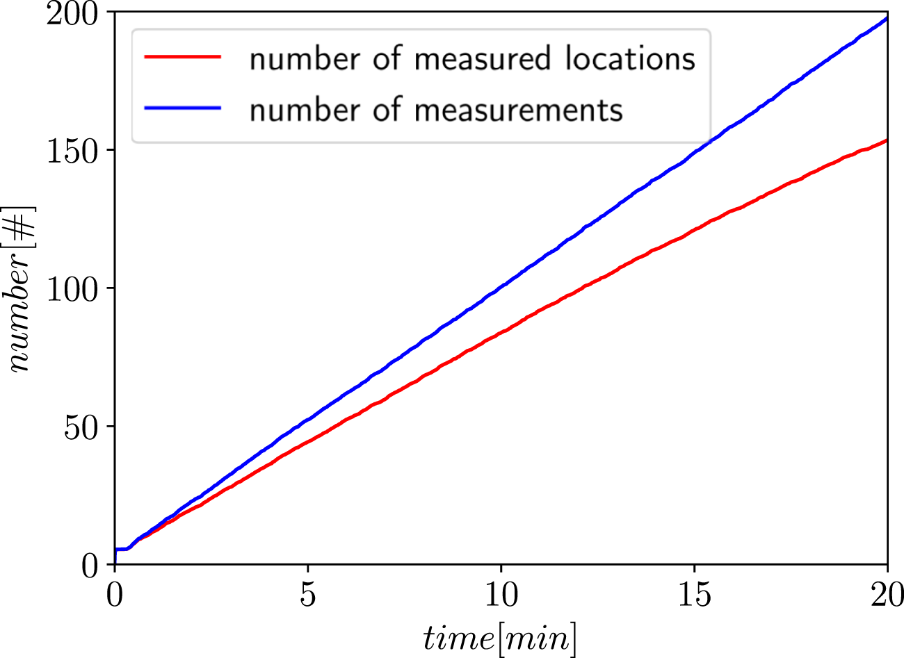

6.1.3. Advantage of model-based approach

At this point, we can conclude from the simulation that the proposed DARE approach generally works and provides an airflow field estimation that is accurate enough in the context of gas source localization. However, here we would also like to compare the approach to a data-driven approach with respect to accuracy to evaluate what we gain from our model assumptions. Therefore, we have chosen a Gaussian Process regression approach as a benchmark. We feed the measurements taken in the 30 simulations depicted in Figure 8(b) (10 for each setup) to a Gaussian Process regression algorithm. We have chosen an implementation based on Rasmussen and Williams (2006) with ⁴ a radial basis function kernel:

$k({\mathit{x}}_a,{\mathit{x}}_b)=e^{-\frac{\Vert {\mathit{x}}_a-{\mathit{x}}_b{\Vert }^2}{2l^2}},$

(24)

with the hyper-parameter l that we tuned manually (l = 0.5 m showed the best performance). This already shows the disadvantage of a Gaussian process, which requires proper training of the hyper-parameter since the performance is highly dependent on it. We consider the airflow components u and v as independent scalar fields and train a separate Gaussian Process for each of them. In Figure 11, we compare the regression capability of the Gaussian process with our domain knowledge-assisted approach based on the Navier-Stokes equations. The error is calculated based on (23), where also for the Gaussian Process only the discretized FEM node positions are evaluated. The curves are averaged over the 30 simulations. As can be seen, our approach always outperforms the Gaussian Process regression, especially in the first minutes when only a few measurements are available. Also, when looking at the worst-case performance (upper limit of the colored areas), the model-based approach outperforms the Gaussian Process. However, with more measurements, the Gaussian process starts to approach the performance of our approach. In addition to the l = 0.5 m, Figure 11 also shows the performance of the Gaussian process for hyper-parameter l = 0.05 m and l = 5 m. As can be seen, the performance degenerates heavily with sub-optimal choices of the hyper-parameter. From this simulation, we can conclude that, as expected, incorporating additional domain knowledge is beneficial for airflow reconstruction.

Figure 11.

The plot compares the regression performance of a Gaussian Process in red with our DARE approach shown in blue averaged over 30 runs. The colored areas indicate maximum and minimum performance for both approaches. In addition, the dotted and dashed lines show the Gaussian Process performance for other values of the hyper-parameter l.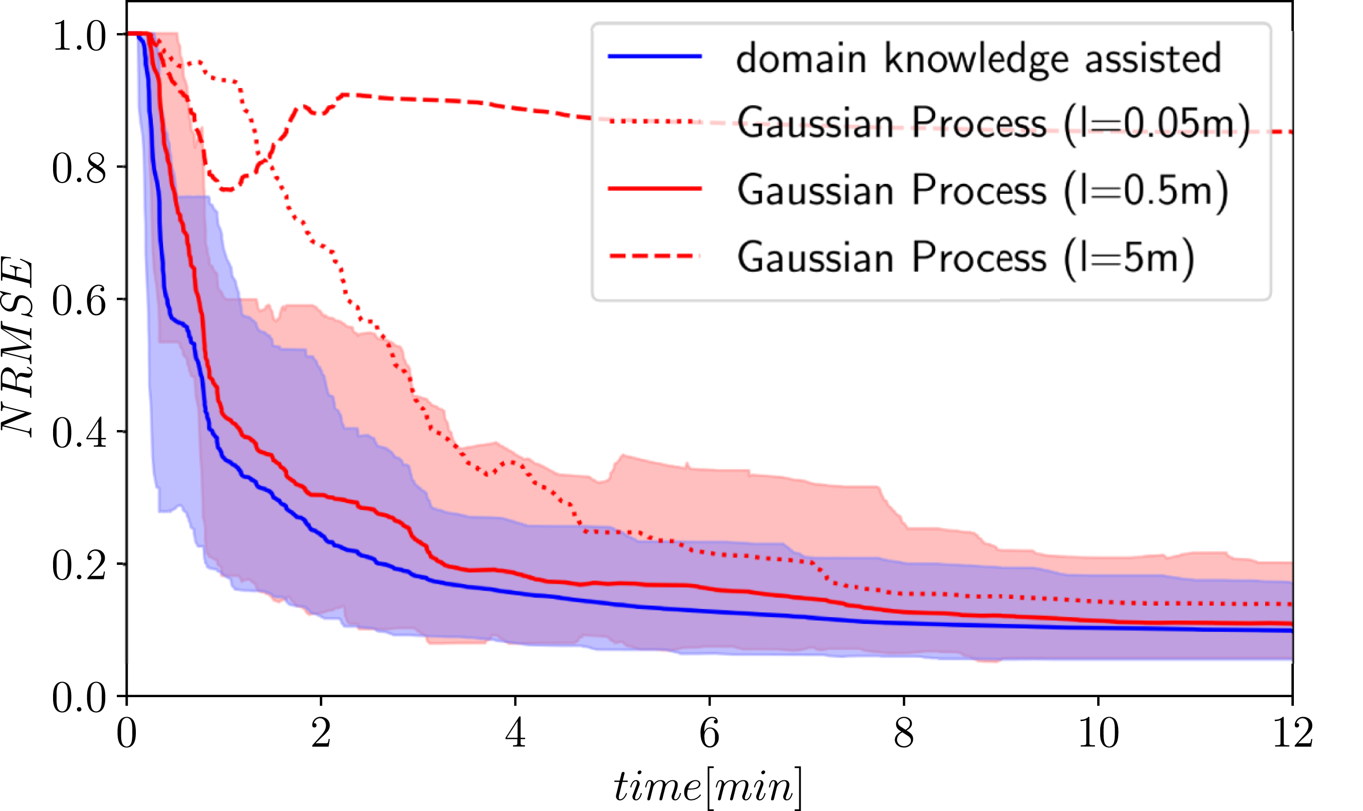

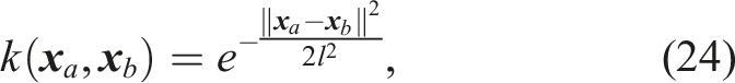
6.1.4. Verification of uncertainty map

In the presented simulation, the robots move according to our uncertainty-driven exploration strategy based on the estimated uncertainty map. In the following, we would like to validate that the calculated uncertainty map actually corresponds to the variances of the marginal distributions of the posterior (see equation (20)). To this end, we consider equations (13)–(15) and the regularization disturbed by a random vector:

$\mathit{M}\mathit{\theta }={\mathit{r}}_1,\mathit{L}\mathit{\theta }={\mathit{r}}_2,\mathit{B}\mathit{\theta }={\mathit{r}}_3,\mathit{I}\mathit{\theta }={\mathit{r}}_4,$

(25)

with the random vectors following the normal distribution, that is, r ₁ ∝ N(0, 1/τ _m I ), r ₂ ∝ N(0, 1/τ _s I ), r ₃ ∝ N(0, 1/τ _b I ), r ₄ ∝ N(0, 1/τ _p I ). We re-scale each equation by the precision:

${\tau }_m\mathit{M}\mathit{\theta }={\widehat{\mathit{r}}}_1,{\tau }_s\mathit{L}\mathit{\theta }={\widehat{\mathit{r}}}_2,{\tau }_b\mathit{B}\mathit{\theta }={\widehat{\mathit{r}}}_3,{\tau }_p\mathit{I}\mathit{\theta }={\widehat{\mathit{r}}}_4,$

(26)

so that the new random vectors on the right side ${\widehat{\mathit{r}}}_{1,\dots ,4}$ follow a normal distribution with variance 1. A least square formulation of these equations corresponds to our posterior distribution (18) in the log domain. We solve the equations in (26) for θ in a least square sense 5000 times with randomly chosen ${\widehat{\mathit{r}}}_{1,\dots ,4}$ . We then calculate the variance of each entry in θ based on the 5000 Monte Carlo runs. For each mesh node i, the corresponding variances of u _i and v _i contained in θ are added up, and the resulting variance map is depicted in Figure 12(a). In addition, Figure 12(b) shows the uncertainty map calculated as explained in Section 4. Both maps are normalized with respect to the highest value occurring in the variance map of the 5000 Monte Carlo runs. As can be seen from the difference between the two maps in Figure 12(c), the maps nearly perfectly match. Please note that the legend is scaled down 60 times compared to Figure 12(b). (With more Monte Carlo runs, we can expect the error to approach zero.) Here, we would like to remark that the results presented in Figure 12 act more as a sanity check and verification of the proposed approach. Of course, one can expect these results, and they are not surprising according to the derivations of Section 3 and Section 4.

Figure 12.

The plots compare the uncertainty map acquired by calculating the variance of multiple Monte Carlo runs in (a) and by the calculation derived in Section 4 in (b). Both maps are normalized with respect to the highest value in (a). The plot in (c) shows the difference between the two maps.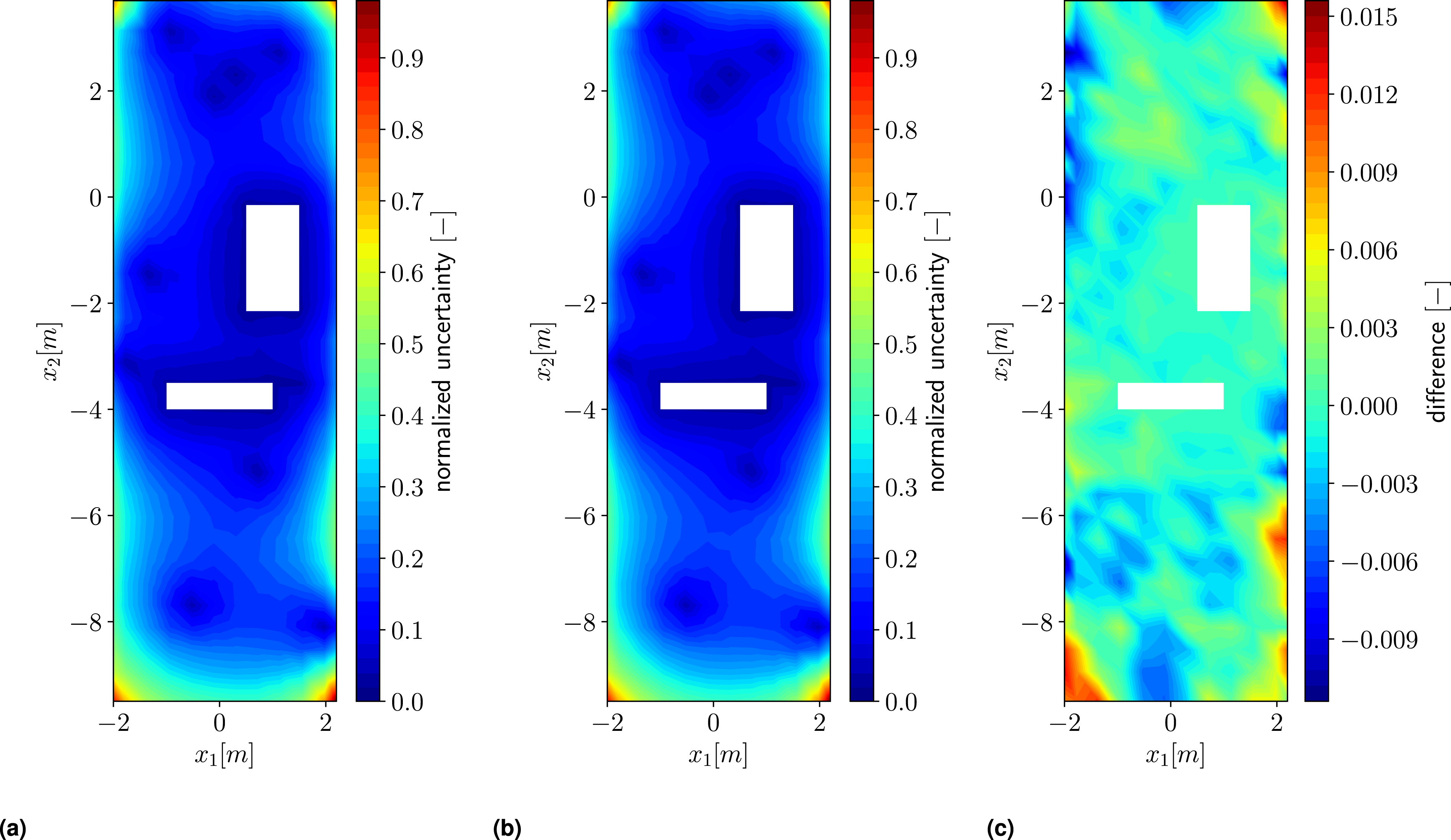

6.1.5. Comparison to random sampling

We also ran 30 simulations (10 for each of the three setups) with a different exploration strategy. This time, the next waypoints are chosen randomly by the robots. However, still following the RRT* path planner to avoid collisions. The performance of this sampling approach is compared to the uncertainty-driven exploration strategy in Figure 13. From the curves in Figure 13(a), it can be seen that, on average, the performance is quite similar. The plot implies that for our setup, a uniform random sampling strategy seems to be a good approach in general. The violin plots in Figure 13(b) illustrate the statistics of the 30 simulations for time steps 2.5, 5.0, 7., and 10.0 min. Here, we can see again that the mean is quite similar. However, the spread of the performance is higher for the random sampling approach compared to the uncertainty-driven exploration. We can interpret these results in the following way: the random sampling approach, by chance, achieves better performance in some simulation runs, yet in other runs, worse performance is achieved. In this respect, the performance of the uncertainty-driven exploration strategy is more consistent and more deterministic throughout the simulations.

Figure 13.

The plots compare the performance of the uncertainty-driven exploration strategy and a random sampling approach. In (a), the NRMSE is plotted over time averaged over 30 simulation runs. The colored areas indicate maximum and minimum observed error in the simulation runs. The violin plots in (b) illustrate a more detailed statistic of the errors for time steps 2.5, 5.0, 7.5, 10.0 min.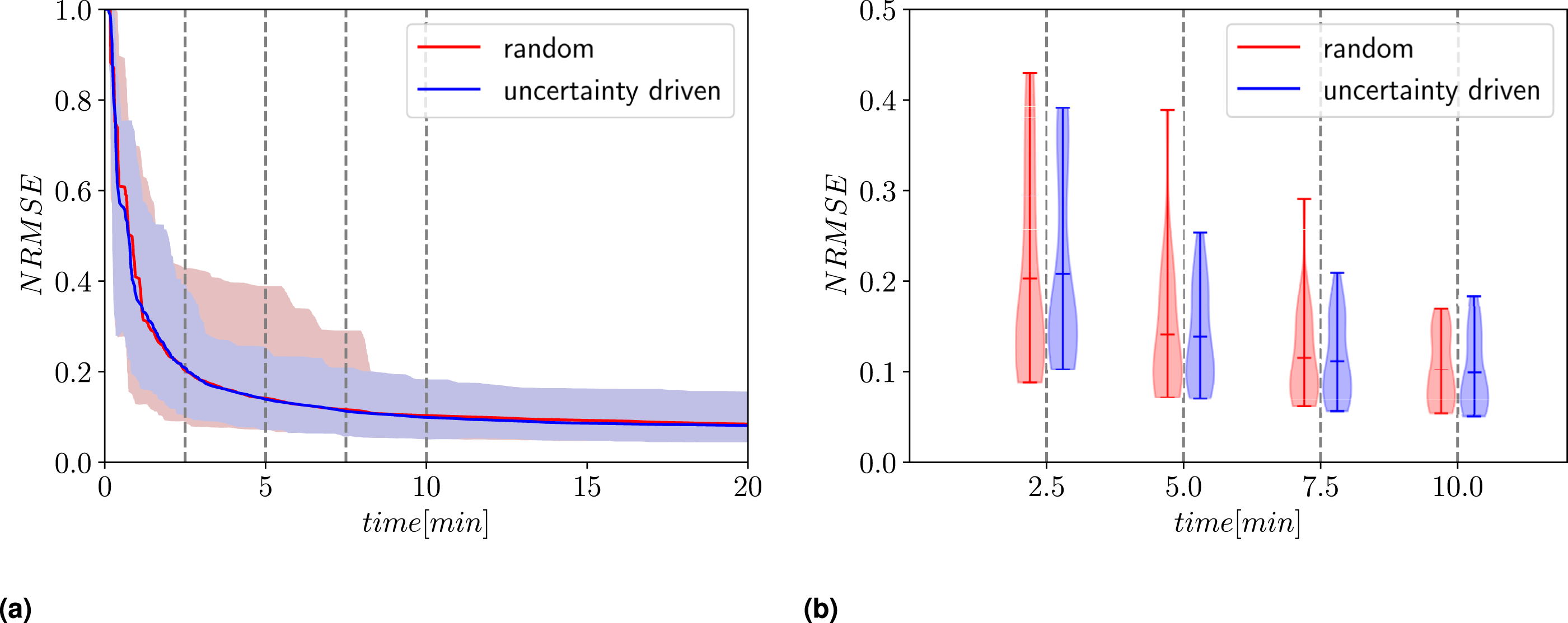

6.2. Laboratory experiments

As proof of concept, we also conducted real-world experiments.

6.2.1. Reconstruction

The experiments were carried out in an area of 4 m times 13 m in an indoor laboratory. We placed two rectangular obstacles Γ_o,1 and Γ_o,2 in the area with sizes 0.5 m × 2.0 m and 1.0 m × 2.0 m at known locations. According to these, we include in our airflow model no-slip boundary condition (w₁( x ) = 0; w₂( x ) = 0; x ∈ {Γ_o,1, Γ_o,2}). The remaining boundary conditions are considered unknown. In addition to a natural airflow in the room due to ventilation and air conditioning, we placed two arrays of fans to generate an additional airflow in the experimental area. The corresponding experimental setup is shown in Figure 14. The location of the obstacles and fans is varied to create different environmental conditions. In all experiments, five robots were used to estimate the airflow map. Now, in contrast to the simulation, the airflow measurements are noisy. In Figure 3, we show the histograms of the collected u- and v-components of the sampled airflow. The main reasons for the quite high variance in the measurements noise are non-steady airflow conditions in the room and small turbulence. It is desirable that in the airflow estimate these effects will be smoothed out.

Figure 14.

Picture of the experimental setup in the laboratory: A video showing the experiment can be found here: https://youtu.be/otn5QMRsve4.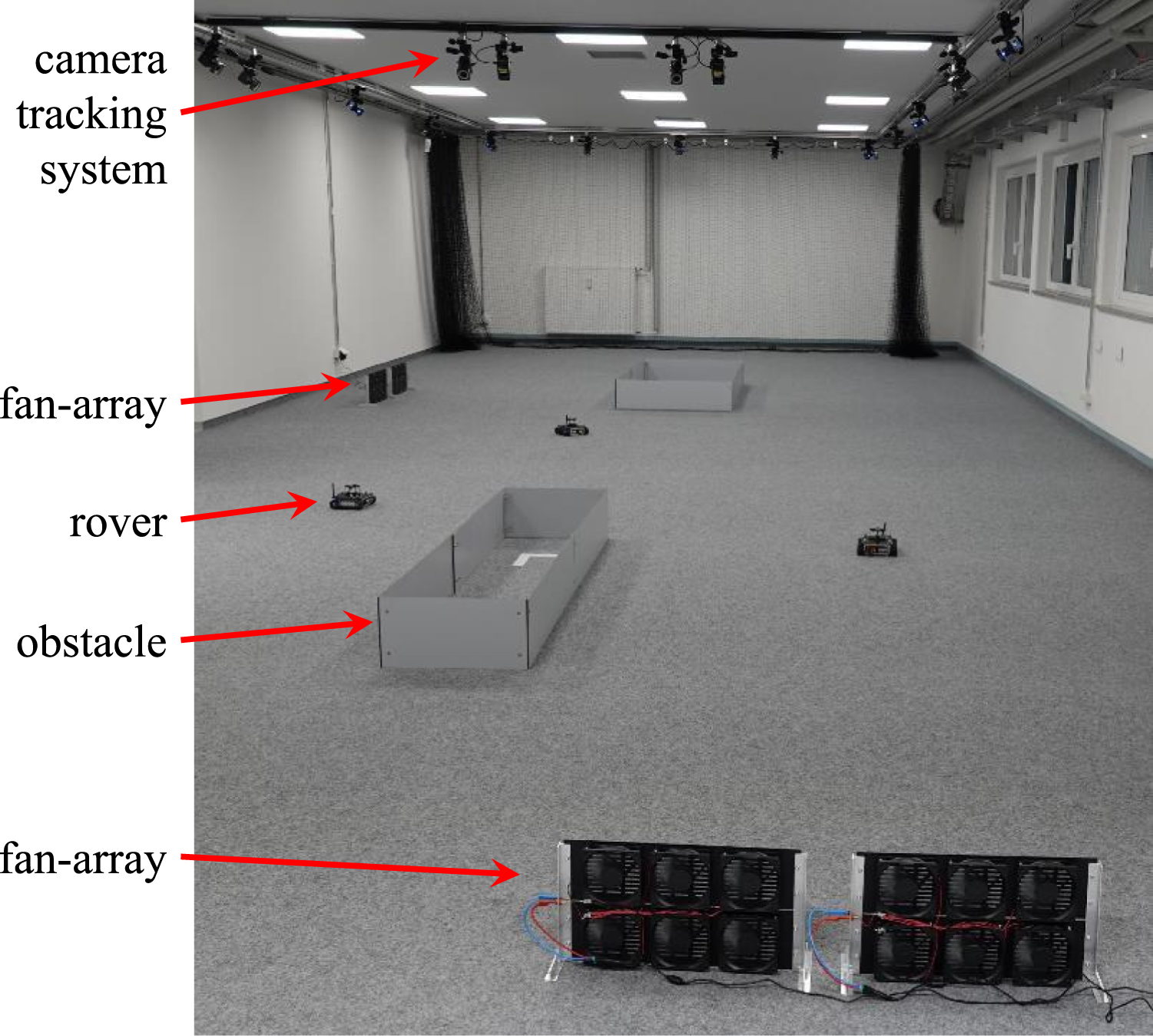

Figure 15 shows snapshots of an experiment. In Figure 15(a), the estimated airflow field is depicted after 2 min and in Figure 15(b) after 10 min, as well as the corresponding uncertainty maps in Figures 15(c) and (d). The obstacles and the fans indicated are at similar locations as in the simulation (see Figure 7). Again, we would like to note that it is impossible to quantify an estimation error here since no ground truth data is available. Nevertheless, the estimated airflow field after 10 min seems reasonable considering results from the simulation in a similar setup. However, the velocity field is more noisy and irregular compared to the simulation (see Figure 7).

Figure 15.

In (a), the estimated airflow field of an experiment after 2 min and in (b) after 10 min are shown. The white stars indicate the measurement locations. The black rectangles mark obstacles, and the red lines at the border are the fans’ locations. In (c) and (d), the uncertainty maps after 2 min and 10 min are depicted.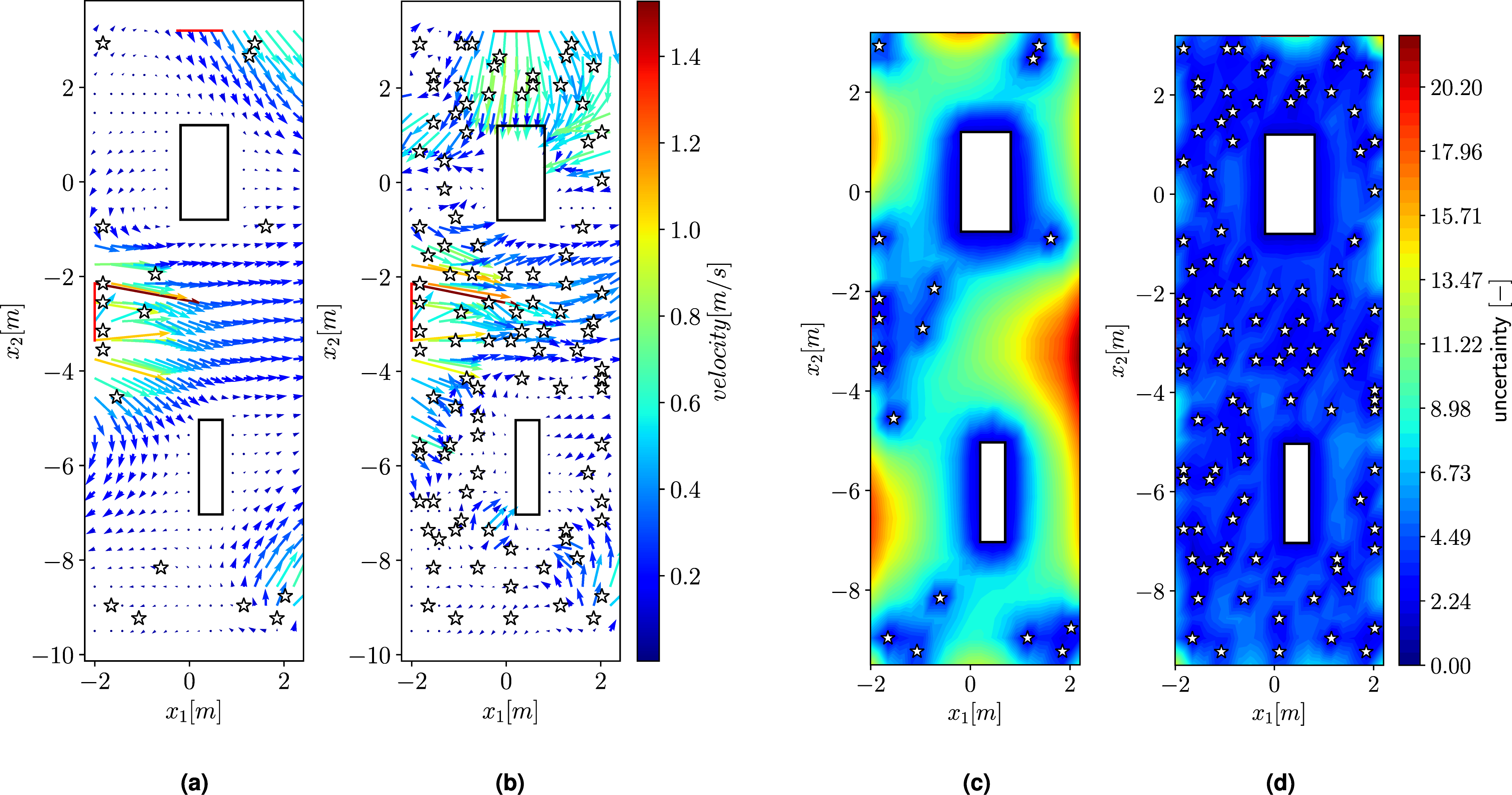

In this context, the parameter τ _m can be used to specify how much impact the measurement noise will have on the solution. So, we had a closer look at the situation after 40 iterations of model updates in a different experiment in Figure 16. To show the influence of the parameter τ _m , three different values were chosen, and the resulting airflow maps are displayed side-by-side. We would like to point out that it is not so much the actual value of τ _m itself that plays a key role, but its ratio to τ _s . In Figure 16(a) the parameter is set to τ _m = 0.001. So, we assume a high measurement noise, that is, a low precision τ _m . This means a low trust or weight of the likelihood compared to the model weighted by τ _s = 1 (see equation (18)). In addition, the regularization term becomes more heavily weighted by τ _p relative to the likelihood. As a consequence, the estimated airflow field appears smoother. In contrast, in Figure 16(c) on the right, the parameter τ _m is set to 1000. This means we trust our measurements and presume a low noise level. In other words, our approach is mostly data-driven. Since real measurements are noisy, this leads to a more “chaotic” and disordered airflow field in Figure 16(c). Furthermore, the airflow field most likely will violate the Navier-Stokes equations, since the model assumptions are less weighted in the reconstruction than the noisy measurements. In Figure 16(b), we set τ _m = 1, which leads to a somewhat averaged case and seems to be a good compromise. The plot is less ordered than in Figure 16(a), but especially in front of the fan clusters, the results fit the expected behavior of the airflow better. At the same time, it is smoother than in Figure 16(c).

Figure 16.

Quiver plots of the estimated airflow field for different values of τ _m : The measurements are exactly the same in all three cases. The black rectangles mark obstacles, and the red lines at the border indicate the locations of the fans. In (a) τ _m is set to 0.001, in (b) to 1 and in (c) to 1000.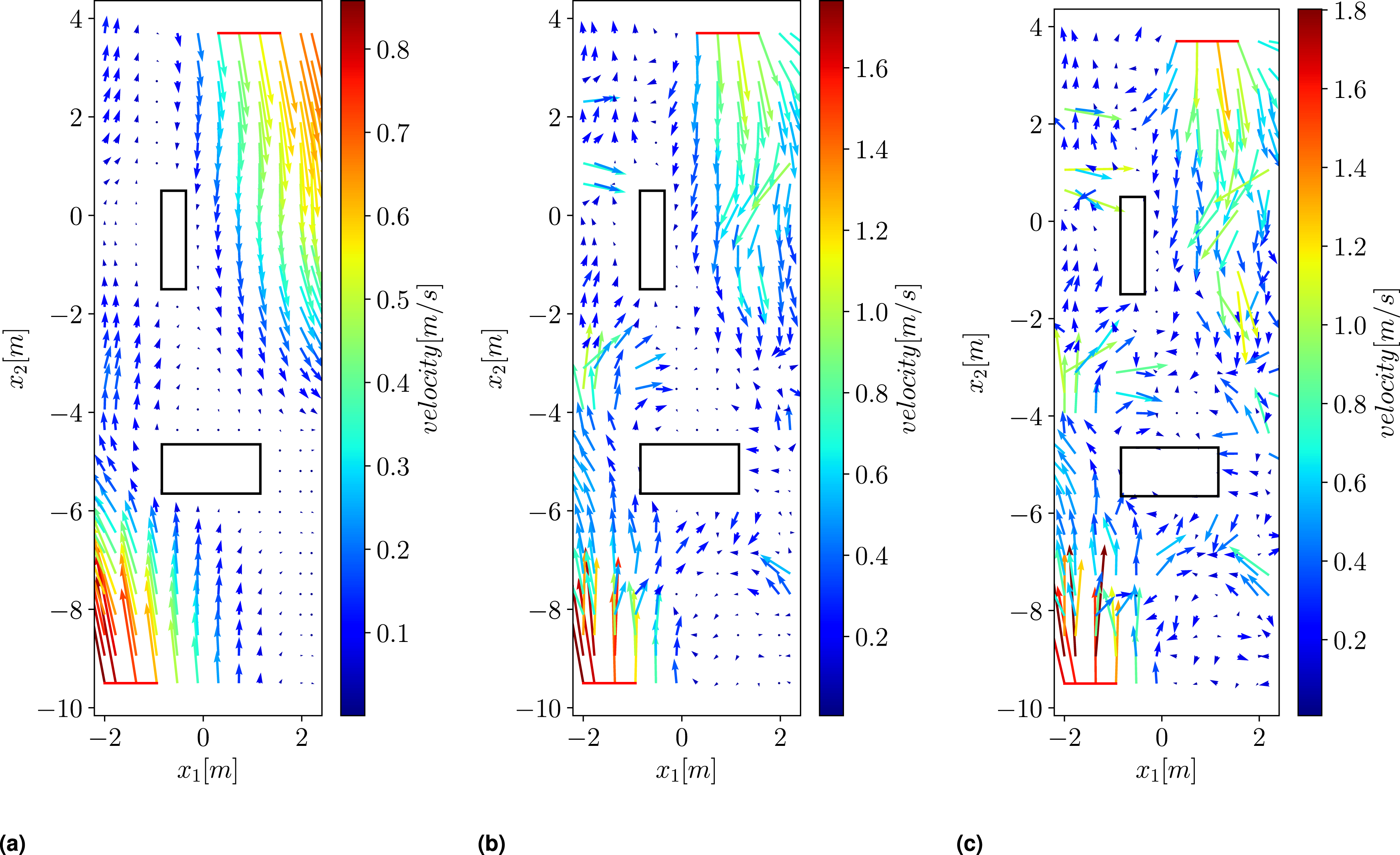

6.2.2. Exploration

In the previous section, we compared the uncertainty-driven exploration strategy to a random sampling approach. Now, as an additional benchmark, we compare the uncertainty-driven exploration strategy with systematic sampling, where the robots follow some predefined paths that cover the whole area. For this, all the possible measurement locations (i.e., mesh nodes) are divided into five clusters, and each cluster is assigned to one robot. By solving the Travelling Salesperson Problem, the locations are ordered in a way so that all points are visited and the traveling time is minimized. The resulting paths for the robots can be seen in Figure 17. This approach has the advantage that measurements are taken at all possible measurement locations. However, the sampling strategy is not intelligent with respect to airflow measurements. So, it might take a long time for the robots to reach informative measurement locations. Consequently, it takes longer to accurately map the airflow. In Figure 18(a), the performance of the full coverage strategy is compared to the proposed uncertainty-driven exploration strategy. Due to the lack of ground truth data in the experiments, the error is calculated with respect to the estimated airflow field at the end of the experiments after 30 min. The plots show clearly that the proposed exploration strategy converges faster to its final results compared to the full coverage approach.

Figure 17.

The plot depicts the predefined trajectories of five robots of the full coverage benchmark strategy.

Figure 18.

In (a), the performance of the proposed uncertainty-driven exploration strategy is compared to a full coverage sampling approach. The error is calculated with respect to the estimated airflow field at the end of the experiment. In (b), the mutual difference between airflow fields estimated in different experiment setups is depicted. The difference is measured by the NRMSE, where one of the experiments is used as a reference for normalization. Three experiments for setup 2 were carried out with the uncertainty-driven exploration and three with the full coverage approach.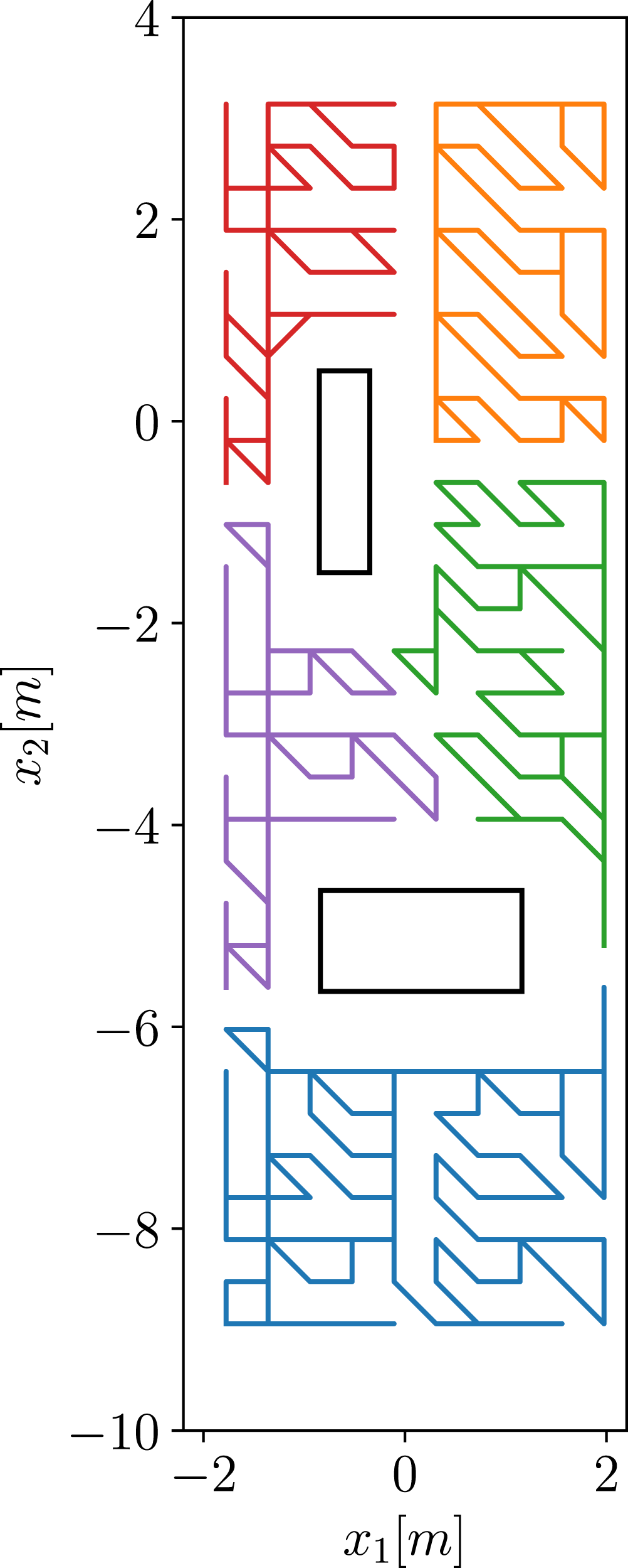

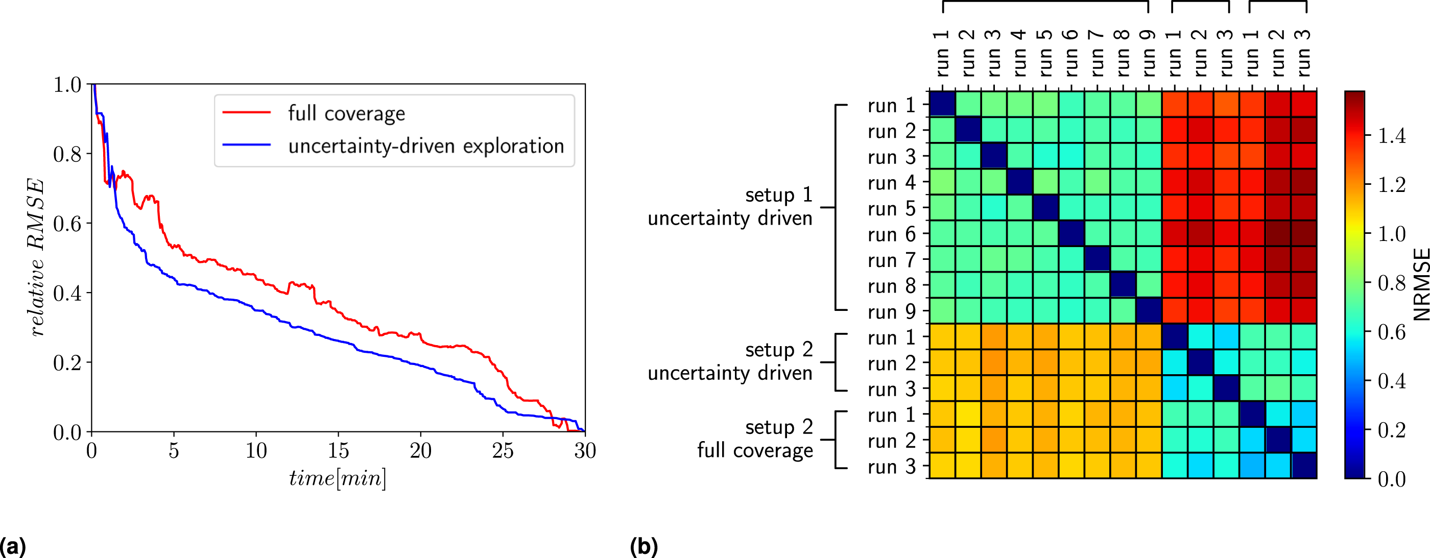
Finally, we would like to compare the results of different experimental runs to evaluate if the estimated airflow maps converge to similar results for the same setup. This comparison is shown in Figure 18(b) for two different setups. In the first setup, nine experiments were carried out with the proposed uncertainty-driven exploration strategy. In the second setup, three experiments were performed by robots following the uncertainty-driven exploration strategy and three experiments following the full coverage approach. For this benchmark, we measured the difference by means of the NRMSE as explained in equation (23), yet the role of the ground truth value is played by one of the experiment results. In Figure 18(b), the differences between the estimated airflow fields at the end of the two experiments are shown for all possible combinations.

Since the error is normalized with respect to one of the experiments, the table is not symmetric. As expected, the error between two experiments with the same setup is significantly lower compared to the difference between the estimated airflow field in different setups. Further, the differences between runs in the same setup are in the same range and independent of the sampling strategy. So, the mutual differences in setup 2 between the uncertainty-driven exploration strategy and the full coverage approach are also in a similar range. This supports the conclusion that the robots actually mapped the airflow field correctly and that the reconstruction works well independently of the exploration strategy.

At this point, we would like to briefly comment on how the proposed approach scales with the number of agents, even though a detailed analysis of this effect is outside the scope of this paper. In general, more agents could collect more measurements at the same time and speed up the exploration process. Computational-wise, the bottleneck is the model update (see Figure 4) and solving the linear equation system for updating the uncertainty map. Fortunately, this step is independent of the number of robots. However, with an increasing number of robots, path planning becomes an issue. Due to the token system and to avoid collisions, only one robot is allowed to plan a path at a time. So, other robots might have to wait. With an increasing number of robots, this waiting (idle) time would become more significant and make the exploration process less efficient.

7. Conclusion

Motivated by applications like gas source localization or gas mapping, where knowledge about airflow is a great advantage, we developed a holistic framework for mapping and exploring 2D airflow fields. Our proposed method enables a multi-robot system to adaptively explore an airflow field where the sampling strategy utilizes domain knowledge encoded by the incompressible Navier-Stokes equations. Due to the adaptive exploration strategy, robots react online to already taken measurements and decide autonomously where to measure next. Therefore, we designed a Bayesian inference framework that allows us to quantify spatial uncertainties of the estimated airflow field and to estimate the spatial airflow field itself by maximizing the corresponding posterior PDF of airflow field parameters. The spatial uncertainty map is then exploited in a robotic path planner for the multi-robot system based on RRT*. Specifically, robots take new measurements in regions with the highest uncertainty, which reduces the total uncertainty of the estimated airflow efficiently. The proposed approach presumes that a priori knowledge about the obstacles in the environment and the currently planned paths from all other robots are available. The swarm acts asynchronously. To this end, a token system was designed to secure the planning phase and ensure that only one robot plans a path at a time. Simulations have shown that the proposed approach can accurately map the airflow field and that the reconstruction works well independently of the exploration strategy. Also, experiments in a laboratory with a swarm of robots equipped with anemometers to sample the air velocity indicate that the airflow reconstruction and the exploration strategy work well. The proposed exploration is more efficient than a predefined full-coverage sampling strategy.

Nonetheless, the discussed approach has some limitations. First of all, especially in outdoor scenarios, the airflow map would not be steady and is generally time-dependent. Therefore, the approach would need to be extended to a time-variant case, which would also imply considering time-dependent Navier-Stokes equations. As a consequence, the complexity of the airflow map estimation problem would increase. Furthermore, the 2D treatment of the airflow field is an oversimplification of reality, especially in indoor scenarios where standard ventilation systems can result in vertical airflow components. Such environments would require a 3D model.

As our primary motivation was gas source localization and gas mapping, coupling airflow exploration with these applications would be a reasonable next step in further work. This opens new, interesting research directions in the context of robotic olfaction. In particular, infotaxis-based approaches similar to the one proposed here will be of interest for coupled models of airflow and gas dispersion to answer questions like: Is a measurement of the airflow at a certain point more informative than a gas concentration measurement at another location?

DARE: Domain knowledge Assisted Exploration

PDE: Partial Differential Equation

CBRN: Chemical, Biological, Radiological and Nuclear

FEM: Finite Element Method

PDF: Probability Density Function

RRT: Rapidly-Exploring Random Tree

NRMSE: Normalized Root-Mean-Square Error

SLAM: Simultaneous Localization and Mapping

MAP: Maximum a Posteriori

Supplemental Material