
Abstract
Computing optimal, collision-free trajectories for high-dimensional systems is a challenging and important problem. Sampling-based planners struggle with the dimensionality, whereas trajectory optimizers may get stuck in local minima due to inherent nonconvexities in the optimization landscape. The use of mixed-integer programming to encapsulate these nonconvexities and find globally optimal trajectories has recently shown great promise, thanks in part to tight convex relaxations and efficient approximation strategies that greatly reduce runtimes. These approaches were previously limited to Euclidean configuration spaces, precluding their use with mobile bases or continuous revolute joints. In this paper, we handle such scenarios by modeling configuration spaces as Riemannian manifolds, and we describe a reduction procedure for the zero-curvature case to a mixed-integer convex optimization problem. We further present a method for obtaining approximate solutions via piecewise-linear approximations that is applicable to manifolds of arbitrary curvature. We demonstrate our results on various robot platforms, including producing efficient collision-free trajectories for a PR2 bimanual mobile manipulator.
1. Introduction
Planning the motion of robots through environments with obstacles is a long-standing and ever-present problem in robotics. In this paper, we aim to find the shortest path between a start and goal configuration with guaranteed collision avoidance. We are particularly motivated by planning for bimanual mobile manipulators, such as the PR2 (Willow Garage). Such robots are well suited for a variety of tasks in human environments but present various challenges for existing motion planning algorithms.
Most popular approaches for this task fall into two categories: sampling-based planners and trajectory optimizers. The trajectory optimization problem is inherently nonconvex when there are obstacles in the scene, so solvers frequently get stuck in local minima. In that case, they may output a path that is longer than the global optimum or even fail to produce a valid path even when one exists.
On the other hand, sampling-based planners can avoid getting stuck in local minima, but the path may be locally suboptimal, resulting in jerky and uneven motion. Sampling-based planners may also suffer from the so-called “Curse of Dimensionality.” Because they rely on covering the configuration space with discrete samples, in the worst case, the number of samples required may increase exponentially with the dimension. The PR2 has two 7-DoF arms and a mobile base, and sampling-based planners struggle with the instances we study here.
Recently, Marcucci et al. (2023) described a new type of motion planning, based on a decomposition of the collision-free subset of configuration space (C-Free) into convex sets. They leverage a new optimization framework, a Graph of Convex Sets (GCS), where each vertex is associated with a convex set and each edge is associated with a convex function (Marcucci et al., 2021). Motion planning becomes a shortest-path problem in this space. This GCS Trajectory Optimization approach (abbreviated as GcsTrajOpt) has been successfully applied to challenging, high-dimensional problems, including bimanual manipulation problems.
However, GcsTrajOpt is limited to Euclidean configuration spaces. A mobile manipulator’s configuration space is inherently non-Euclidean due to the mobile base: the robot can rotate through a full 360°, and its configuration is identical to when it started. Continuous revolute joints present a similar issue. Although the configuration spaces of interest are inherently non-Euclidean, they are still “locally” Euclidean, leading to elegant descriptions as differentiable manifolds. With a Riemannian metric, which allows one to measure distance on a manifold, the concepts of convexity generalize to nonlinear spaces. This in turn allows optimization on manifolds with rigorous guarantees, analogous to those obtained from convex optimization on Euclidean spaces.
A conference version of this paper is published in Cohn et al. (2023). This manuscript extends the results to more general classes of robot configuration spaces via a piecewise-linear approximation. This encompasses closed kinematic chains, whose configuration spaces can naturally be represented as the (generally nonconvex) feasible set of a system of nonlinear equality constraints. This also allows planning over the group of 3D rotations, enabling our method to handle ball joints and free bodies. (The approximation strategy is required in this case due to the inherent nonconvexity of the distance function; see Subsection 6.5 for details).
In this paper, we formulate the general problem of shortest-path motion planning around obstacles on Riemannian manifolds. We define a graph of geodesically convex sets (GGCS), the analogue to GCS on a Riemannian manifold. We prove that this formulation has all the requisite properties needed to inherit the same guarantees as (Euclidean) GCS for a certain class of robot configuration spaces, encompassing open kinematic chains with continuous revolute joints and mobile bases. In this case, our theoretical developments lead to simple and elegant modifications to the original GcsTrajOpt. We entitle this generalization GGCS Trajectory Optimization (abbreviated as GgcsTrajOpt), and demonstrate its efficacy with several challenging motion planning experiments.
2. Related work
In the world of continuous motion planning around obstacles, most popular techniques fall into two categories: sampling-based planners and trajectory optimizers.
Sampling-based motion planners partially cover C-Free with a large number of discrete samples. Two of the foundational sampling-based planning algorithms are Probabilistic Roadmaps (PRMs) (Kavraki et al., 1996) and Rapidly-Exploring Random Trees (RRTs) (LaValle, 1998). Such algorithms are probabilistically complete, that is, with enough samples, they will always find a valid path (if one exists). However, these algorithms are only effective if a valid plan can be produced with a reasonable number of samples. Hence, the “curse of dimensionality” is a potential obstacle to sampling-based planning, and such techniques have struggled with high-dimensional problems such as bimanual manipulation. In most cases, planning for bimanual tasks is accomplished by planning for one arm, then planning the second arm independently while treating the first arm as a dynamic obstacle. This is a reasonable heuristic for some tasks, but it sacrifices even probabilistic completeness.
An alternative approach is to formulate motion planning as an optimization problem. This requires parametrizing the space of all trajectories and defining constraints and cost functions that describe the suitability of each trajectory. Examples of kinematic trajectory optimization include B-spline parametrizations using constrained optimization (Tedrake, 2022, §7.2), CHOMP (Zucker et al., 2013), STOMP (Kalakrishnan et al., 2011), and KOMO (Toussaint, 2014). Trajectory optimization approaches do not suffer from the curse of dimensionality, and are suitable for much more complex robotic systems. But the optimization landscape is inherently nonconvex, so trajectory optimization methods cannot guarantee global optimality, and often fail to produce feasible trajectories altogether.
The use of mixed integer programming (MIP) to solve motion planning problems to global optimality has recently seen an increase in popularity as new theoretical results, greater computational resources, and powerful commercial solvers (Gurobi Optimization LLC, 2023; MOSEK ApS, 2019) have been brought to bear. The survey paper of Ioan et al. (2021) provides an overview of the use of MIP in motion planning. Besides the work of Marcucci et al. (2021), Landry et al. (2016) used MIP to plan aggressive quadrotor flights through obstacle-dense environments. MIP has been used to plan footstep locations for humanoid robots (Deits and Tedrake, 2014) and for quadrupeds (Aceituno-Cabezas et al., 2017; Valenzuela, 2016). Dai et al. (2019) used MIP to globally solve the inverse kinematics problem. Finally, MIP has seen extensive use in hybrid task and motion planning (Adu-Bredu et al., 2022; Chen et al., 2022; Saha and Julius, 2017; Tika et al., 2022; Yi et al., 2022).
Mixed integer programs can take a long time to solve in the worst case, but it is often possible to mitigate this problem with appropriate relaxations or approximations (Marcucci et al., 2023; Suh et al., 2020). GCS in particular uses an MIP formulation with a small number of integer variables, making branch-and-bound tractable. Furthermore, the convex relaxation is tight, enabling efficient approximation by solving only a convex problem combined with a randomized rounding strategy. Marcucci et al. (2023) argued that for single-arm manipulators, this approach can find more optimal plans in less time than PRMs. These valuable properties carry over to our extension of GCS.
Another recent trend in motion planning has been the use of Riemannian geometry to model the problem. Riemannian Motion Policies (RMPs) (Ratliff et al., 2018) combine acceleration-based controllers across different task spaces into a single unified controller. A Riemannian metric in each task space determines the priority of a given controller, and smooth maps between the manifolds enable the averaging of controllers. RMPs have seen continued improvement (Cheng et al., 2018; Rana et al., 2021) and generalization (Bylard et al., 2021; Van Wyk et al., 2022). However, RMPs and their extensions are still known to struggle with local minima, similar to nonconvex trajectory optimizers. Klein et al. (2022) envision Riemannian geometry as a tool for generating and combining elegant motion synergies for complex robotic systems.
One can solve optimization problems in these spaces with rigorous guarantees by using a generalization of convexity to Riemannian manifolds, called geodesic convexity (g-convexity). Unfortunately, existing research into g-convex optimization often focuses on specific classes of manifolds that do not encompass the configuration spaces of interest (Bacak, 2014; Zhang and Sra, 2016). In addition, there is little existing literature studying mixed-integer Riemannian convex optimization, and techniques commonly used in the Euclidean case, such as cutting planes (Marchand et al., 2002), may not generalize to Riemannian manifolds.
3. Preliminaries
In this section, we cover some of the relevant mathematical background. We supply intuitive definitions; for further reference on Riemannian geometry, see the textbooks of Do Carmo (1992) and Lee (2013, 2018). Boumal (2022) provides an excellent treatment of optimization over manifolds. We use the notation
3.1. Riemannian geometry
A d-dimensional (topological) manifold

A collection of charts whose domains cover the manifold is called an atlas. We only consider
For each
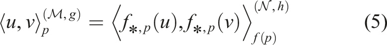
A Riemannian metric g is a smoothly-varying positive-definite bilinear form over
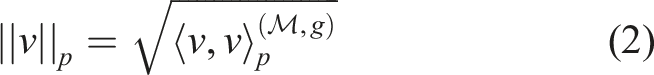
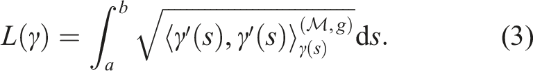
We call the integrand the speed of γ. The distance between any two points
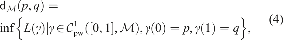
If
A geodesic is a locally length-minimizing curve, parameterized to be constant speed. Locally length-minimizing means that for two points on the geodesic that are close enough, the geodesic traces out the shortest path between them. For example, geodesics in Euclidean space with the natural metric are lines, rays, and line segments, and geodesics on the sphere (with the induced metric from Euclidean space) are great circles. Constructing the shortest geodesic between two points is a variational calculus problem, so the solution must satisfy the Euler–Lagrange system of differential equations. Thus, initial conditions
A Riemannian metric induces curvature on a manifold, capturing how local geometry differs from the standard Euclidean case. The sectional curvature at a point p is a real-valued function defined on two-dimensional subspaces of the tangent space Examples of geodesic triangles T
i
in manifolds 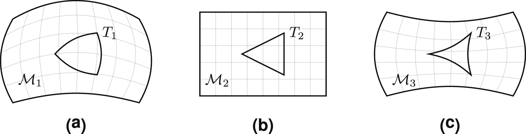
The Cartesian product of two Riemannian manifolds is itself a Riemannian manifold. The curvature of the component manifolds influences the curvature of the product. Importantly, the product of flat manifolds is flat (Atceken and Keles, 2003). As we explain in Section 5, this implies that a robot with a mobile base and (potentially many) continuous revolute joints has a flat configuration space.
3.2. Convex analysis on manifolds
To define convexity on a Riemannian manifold
G-convex neighborhoods exist around every point (Do Carmo, 1992: 77). For any

A function

The primary manifolds of interest in this paper are compact, which presents a major obstacle to using g-convexity. If
We say that f is locally g-convex if for any
3.3. Shortest paths in graphs of convex sets
A Graph of Convex Sets is a directed graph G = (V, E) together with associated convex sets
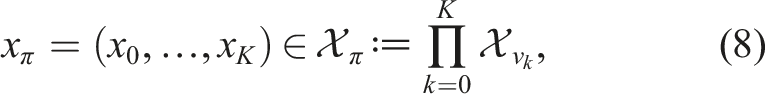
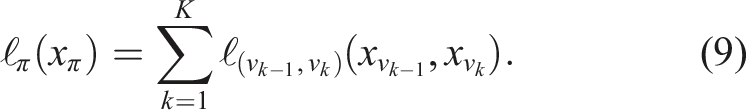
If we let Π describe the set of paths from p to q, then the shortest path problem on a graph of convex sets can be concisely stated as

This formulation implicitly admits edge constraints of the form
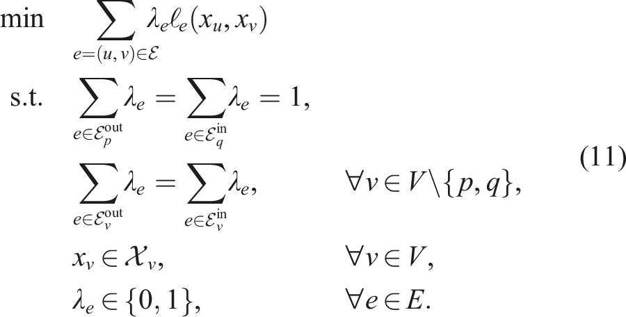
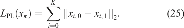
Marcucci et al. (2021) presented a mixed-integer nonlinear programming (MINLP) formulation of this problem, and then constructed a tight mixed-integer convex reformulation. The MINLP formulation builds upon the standard formulation of a graph shortest path problem as a network flow problem (Hillier and Lieberman, 2015: 387). Associate to each e ∈ E a flow variable
When this problem is solved to optimality, the nonzero flow variables will describe a path π, and the corresponding x π will be optimal for (10).
The product terms λ
e
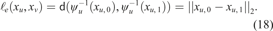
ℓ
e
(x
u
, x
v
) make the objective function nonconvex. Marcucci et al. (2021) describes a tight mixed-integer convex reformulation of (11), which can be handled by standard mathematical optimization solvers, including Gurobi Optimization LLC (2023) and MOSEK ApS (2019). Furthermore, the convex relaxation of this MICP (obtained by replacing the constraints
Building off of this fact, Marcucci et al. (2023) presented a heuristic strategy for quickly obtaining suboptimal solutions. If the optimal value of each flow variable (from the convex relaxation) is interpreted as the likelihood that the shortest path traverses that edge, one can obtain candidate paths via a randomized depth-first search. For each candidate path π, one solves a small convex program to determine the optimal x π , and the best such path is returned. This approach generally produces high quality trajectories for motion planning problems, although they may not be globally optimal.
4. Problem statement
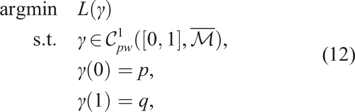
We may now precisely state our kinematic planning problem in the language of Riemannian geometry developed thus far. Let
Suppose we want to find the shortest path between two points p and q in
5. Graphs of geodesically convex sets
We now introduce a graph of geodesically convex sets (GGCS), a Riemannian optimization framework that, in Section 6, we show is general enough to encompass Problem (12). A GGCS is a directed graph G = (V, E) with certain properties, designed as a generalization of ordinary (Euclidean) GCS from Marcucci et al. (2021, §2) to Riemannian manifolds. The definition of a GGCS closely mirrors that of a GCS, as described in Subsection 3.3. Each vertex v ∈ V has a corresponding g-convex subset
Given distinct source and target vertices p, q ∈ V, a path π from p to q is a sequence of distinct vertices
Let Π denote the set of all paths from p to q, and for any π ∈ Π, define its feasible vertices as
Solving Problem (14) to optimality is intractable in complete generality, so we propose to transform it into an ordinary GCS problem. To each v ∈ V, associate a chart ψ
v
, and define

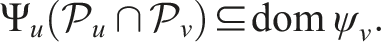
This construction is shown in Figure 2. To apply the GCS machinery, we require that the sets Moving edges and sets from Riemannian manifolds to Euclidean spaces with coordinate charts. In this diagram, 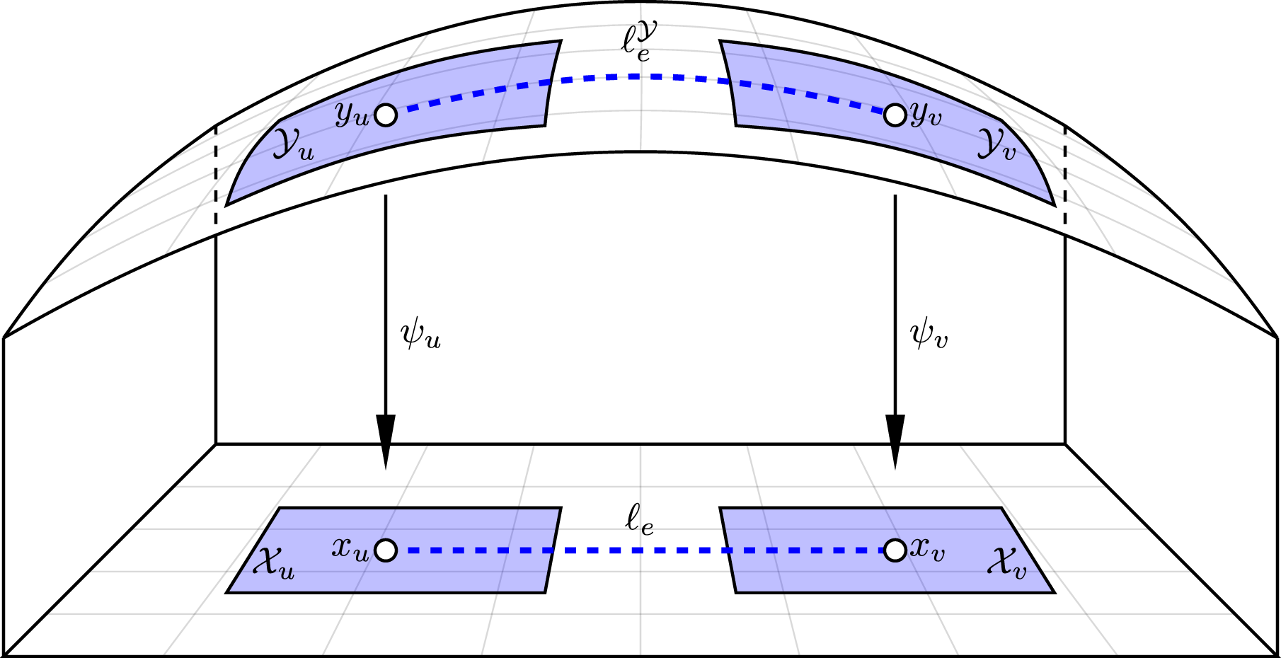
Importantly, many robot configuration spaces can be realized as flat manifolds. SE (2) is flat, all one-dimensional manifolds are flat (Lee, 2018: 47) (this encompasses continuous revolute joints), and products of flat manifolds are flat. Thus, any robotic system whose configuration can be described using a series of single-degree-of-freedom joints (and potentially a mobile base) will have a flat configuration space, and thus can be handled by our methodology. 2-DoF universal joints can also be handled, as they can be perfectly represented as two juxtaposed 1-DoF joints. 3-DoF ball joints cannot be handled perfectly, because decomposing a ball joint into 1-DoF joints distorts the underlying geometry. Instead, one can use a piecewise-linear approximation of this configuration space—see Subsection 6.5 for further discussion. The configuration spaces of certain closed linkages can be explicitly represented as a flat manifold; one constructs a parametrization, and defines the metric on the manifold as the pushforward of the metric in Euclidean space Cohn et al. (2024). Like decomposing a ball joint into 1-DoF revolute joints, this distorts the underlying geometry, so the optimal solutions of the resulting GGCS problem will not be the true shortest paths according to the original metric.
6. Motion planning with GGCS
We want to use GGCS to make motion plans on Riemannian manifolds by solving Problem (12). Thus, we must prove that the optimal value is achieved by some trajectory that is feasible for a GGCS problem. We use the initialism ROSC (Riemannian Open Subset Closure) to describe closures of open subsets of Riemannian manifolds, notably
The proof follows by verifying that
We are given a finite atlas These requirements will not hold in general, but we will discuss how to construct such an atlas in Subsection 6.2. With this information, we can prove a strong result about the shortest paths in
• • γ* is a piecewise geodesic of • Each geodesic segment is contained in some • γ* passes through each
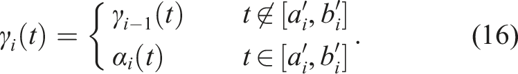
Let γ0 be a continuous minimizing path connecting p to q (guaranteed to exist by Theorem 1); we will use this to construct an appropriate γ*. Select an arbitrary order For each i, if γi−1 does not pass through
6.1. Formulation as a GCS problem
To transform the GGCS problem into a GCS problem, we require that the sets and edge costs are convex in Euclidean space. The following is sufficient (and still encompasses robots with mobile bases and continuous revolute joints):
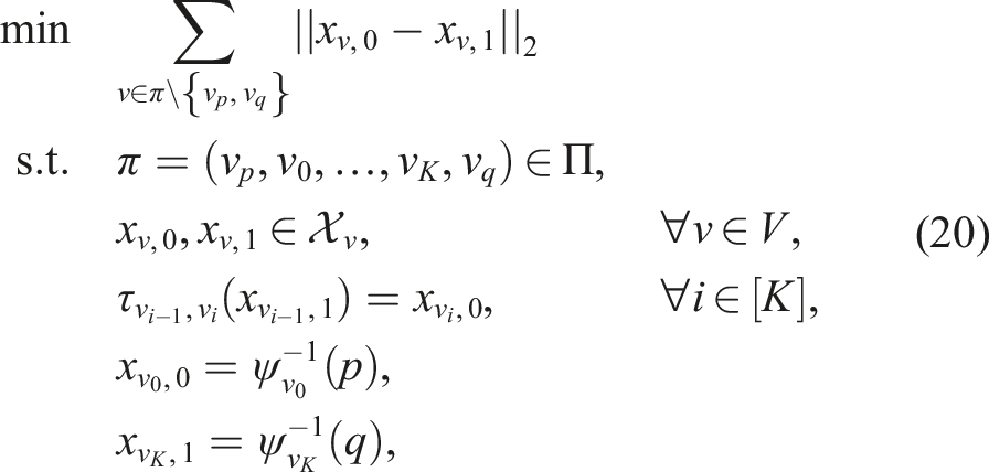
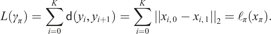
Assumptions 1 and 2 together yield three important results: • • • τu,v is a Euclidean isometry (see Lemma 4 in Appendix A.2), and hence affine (Väisälä, 2003). The first two results are true because To formulate the problem with GCS, we follow an approach similar to Marcucci et al. (2023), where decision variables describe line segments contained within each convex set. For each set Recall that edges are directed, so if two sets This will ensure that the optimal solution has minimal arc length among all possible feasible trajectories, as shown in Theorem 3. We also encode equality constraints to ensure the endpoints of adjacent segments are in agreement: This constraint is convex because τu,v is affine. Let Altogether, the sets and edges above describe the following GCS problem: By using the relaxation strategy of Marcucci et al. (2021), (20) can be solved as a mixed-integer convex program. Alternatively, it can be solved approximately by solving the convex relaxation and using a randomized rounding strategy (Marcucci et al., 2023). After solving the GCS problem, we obtain a path For each


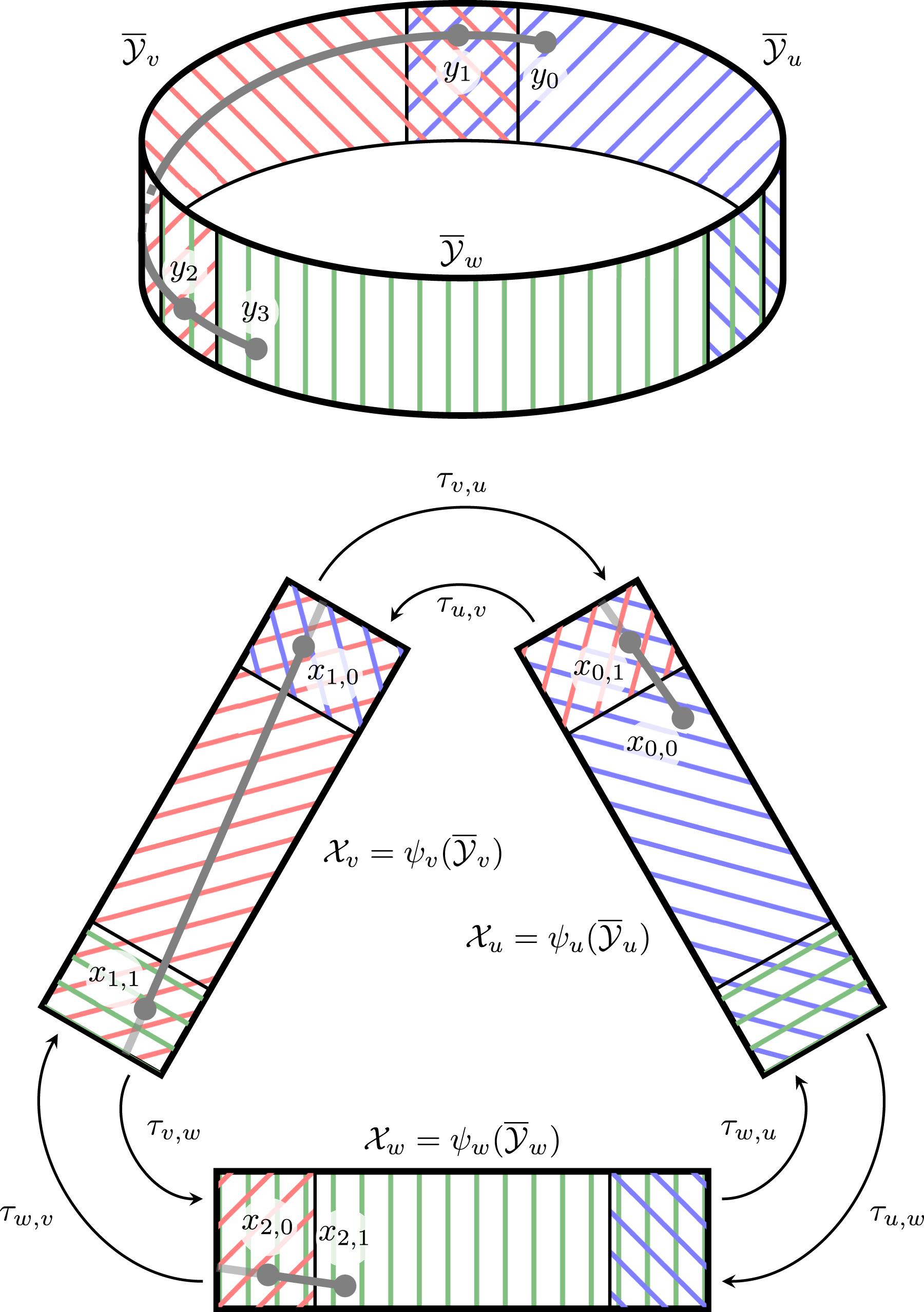
The process of transforming a GGCS problem into a GCS problem for a simple cylinder manifold. Each of the three charts maps to a Euclidean space, with transition maps encoding the equality constraints across chart domains. The line segments then lift to a piecewise geodesic on the manifold.
The proof strategy is as follows. First, we show that feasible solutions to the GCS problem have cost greater than or equal to the optimal solution for Problem (12). Then, we show that optimal solutions for Problem (12) are feasible solutions to the GCS problem. Thus, optimal solutions to the GCS problem are optimal solutions to Problem (12). In particular, any feasible path x
π
for the GCS problem yields a piecewise continuously differentiable curve γ
π
whose image is contained in Thus, the optimal value of Problem (12) is no worse than the optimal value of the GCS problem. Now, consider an optimal γ* for Problem (12), with the properties of Theorem 2. Then γ* is the concatenation of geodesics γ1, …, γ
K
, where

6.2. Construction of the atlas
A key part of motion planning with GGCS is the construction of an appropriate atlas
As in Marcucci et al. (2023), we construct an inner approximation of C-Free using the extension of IRIS (Amice et al., 2023, Alg. 2) to handle nonconvex obstacles. This algorithm takes in a “seed” point and grows a convex collision-free polytope around it, but it is only applicable to robots with joint limits. Given a seed point in
To ensure the set is g-convex when lifted to
Consider the case of the cylinder manifold
For revolute joints without limits and the rotational degree of freedom of mobile bases, the convexity radius is π/2 (as their configuration space is precisely
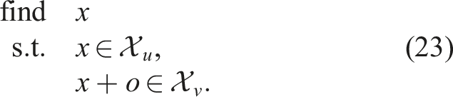
Suppose Given two regions If such an o exists, we then solve the small convex program If such an x exists, then the regions overlap, and their transition map is x
u
↦x
u
+ o. If no such offset exists, or if (23) returns infeasible, then the regions do not overlap. We also assumed full coverage of In general, the computational complexity of the resulting GCS problem grows with both the number of g-convex sets and the density of their overlap graph. So atlases with fewer, larger sets generally lead to faster solve times. Methods used for generating individual convex subsets of C-Free generally attempt to maximize the volume of the resulting sets (Amice et al., 2023; Deits and Tedrake, 2015; Petersen and Tedrake, 2023; Yang and Lavalle, 2004). Werner et al. (2024) attempt to construct an inner covering of an arbitrarily high fraction of C-Free with as few convex sets as possible. Wu et al. (2024) attempt to cover the part of C-Free surrounding a known collision-free trajectory, toward improving that path. In general, building an approximation of C-Free that is ideal for motion planning is an area of active research that is beyond the scope of this paper.
6.3. Additional costs and constraints
Marcucci et al. (2023) extended GcsTrajOpt to parametrize trajectories as piecewise Bézier curves, in order to handle a greater variety of costs and constraints. This includes penalizing the duration and energy of a trajectory, adding velocity bounds, and requiring the trajectory to be differentiable a certain number of times. Bézier curves generalize naturally to Riemannian manifolds by interpolating along the minimizing geodesics between control points (Park and Ravani, 1995; Popiel and Noakes, 2007). Because we restrict ourselves to flat manifolds, the local geometry is unchanged from Euclidean space. Thus, all costs and constraints that operate on individual segments of the piecewise Bézier curve trajectory can be used with no changes.
To enforce the differentiability of the overall trajectory where two segments connect, we must compare tangent vectors across different coordinate systems. In particular, suppose we need differentiability η times for an edge (i, j), with transition map τi,j. Let γ
i
and γ
j
be adjoining Bézier curve segments in

Because the transition map is a Euclidean isometry, its pushforward is a linear transformation described by an orthogonal matrix, and if the coordinate systems are globally aligned (as described in Subsection 6.1), then the pushforward is the identity map. When
6.4. Beyond flat manifolds
The guarantees afforded by GgcsTrajOpt derive from Assumptions 1 and 2. Assumption 1 affects the completeness and optimality of the algorithm, and it may be impossible to construct an appropriate atlas if the boundary of
Assumption 2 is used to guarantee that the resulting optimization problem is convex; without it, we may have nonconvex costs or constraints, and can make no guarantees of finding an optimal (or even feasible) solution. But many manifolds of interest in robotics do not satisfy these requirements. Certain configuration spaces are inherently not flat manifolds. Examples include SO(3), which is the configuration space of a ball joint and SE(3), which is the configuration space of a free rigid body. Planning problems where general kinematic or dynamic constraints have been imposed can also yield a constrained configuration space as an embedded non-flat submanifold of the full configuration space.
6.4.1. Piecewise-linear approximations
To handle arbitrary manifolds, we turn our attention to piecewise-linear (PL) approximations. In particular, we consider a triangulation of the manifold: a simplicial (or polytopic) mesh of appropriate dimension whose topology matches the manifold. For certain known manifolds, obtaining PL approximations is straightforward; for example, one can tessellate the two-sphere by iteratively subdividing the faces of an icosahedron, and lifting the new vertices to the surface (Dahl et al., 2014, §2.B.1). For an arbitrary manifold which has a known atlas, one can tessellate the image of each chart in Euclidean space, and lift that tessellation to the manifold (Cohn et al., 2022). For implicitly defined manifolds, there is extensive literature on the method of continuation, where a single point known to lie on the manifold is used to generate an explicit PL approximation (Dankowicz and Schilder, 2013; Ghosh, 2012; Henderson, 2002). Continuation in particular has been successfully integrated with sampling-based motion planning algorithms, in order to solve motion planning problems with nonlinear equality constraints (Porta and Jaillet, 2010).
The GCS machinery can be used to plan along a PL approximation; indeed, the original GCS paper directly considers piecewise-affine systems (Marcucci et al., 2021, §9.3). In the context of approximating a smooth manifold, we will treat each simplex as a chart domain, replace the transition map with the mapping between two adjacent simplices, and approximate the arc length on the manifold with the arc length along the PL approximation.
We consider a similar problem setup to Jaillet and Porta (2013). The configuration space
Given an atlas of
We cannot satisfy Assumption 2, as
We will leverage this fact in the procedure for lifting a path x
π
in the PL approximation to a path y
π
on
Solving the shortest path problem on the PL approximation yields a path x
π
as in (21). However, we generally do not have Ψ
u
(xu,1) = Ψ
v
(xv,0), so the process for lifting to a path y
π
on

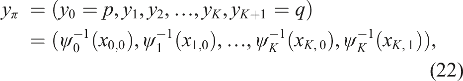
Overall, solving the shortest path problem gives us a path (x0,0, x0,1, …, xK,0, xK,1), where xi−1,1 = xi,0 for each i ∈ [K]. We lift it to a sequence of waypoints (y0,0, y0,1, …, yK,0, yK,1), where we may have yi−1,1 ≠ yi,0 for some i ∈ [K]. Finally, for each i ∈ [K], if it would be shorter to skip yi,0 and go straight from yi−1,1 to yi,1, we drop yi,0 from the path. Such a “skip” occurs when paths along the PL approximation are longer than those along the manifold. As an example, consider a circle manifold, inscribed within a regular hexagon (which serves as the PL approximation). If a path along the hexagon were projected onto the circle, then traversing from yi−1,1 to yi,0 would require doubling back—the path is shorter if one goes straight from yi−1,1 to yi,1.
We now endeavor to prove this GCS problem provides a useful approximation of Problem (12). We introduce the following notation to describe the length of a path along the PL approximation:
The PL approximation then becomes a metric space with distance function
We will provide an upper bound on • ϵ
H
: The maximum chart Hausdorff distance • αmax: The largest principal angle (Knyazev and Zhu, 2012) between any pair of adjacent charts.
Hausdorff distance is a common metric to quantify the difference between two approximations of a geometric object (Cignoni et al., 1998). The largest principal angle between charts, together with the radius of the smallest chart, presents a coarse bound on the curvature of the manifold. Taking a finer discretization generally leads to both quantities decreasing; for example, see Figure 4. Furthermore, compactness of the manifold ensures that the curvature is bounded, so ϵ
H
and αmax can be made arbitrarily small with finitely many charts. A shortest path problem on the unit sphere solved with GgcsTrajopt using an increasingly fine discretization. The blue and green markers denote the start and end configurations, respectively. The solid black path denotes the shortest path along the mesh (found with GgcsTrajOpt), and the dotted black path is the result obtained when that path is lifted back to the sphere. Conversely, the red dotted path is the ground truth shortest path along the sphere, and the solid red path is its projection onto the PL approximation.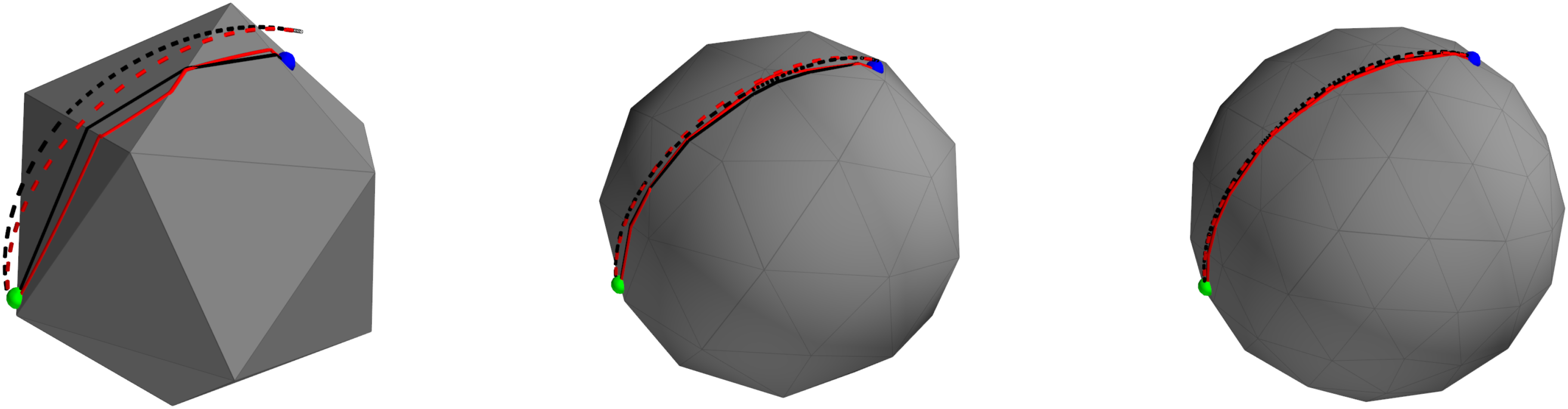
We leverage two lemmata in deriving a global upper bound on the path length (see proofs in Appendix A.3).
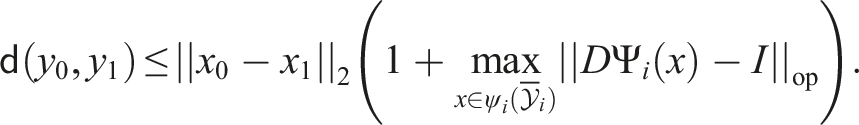
Fix a chart This demonstrates that the error within a chart is upper bounded by how much the total derivative of the chart mapping deviates from the identity mapping. When constructing charts as in Jaillet and Porta (2013), the polytope is constructed so as to lie along the tangent space of some point on the manifold. Thus, there is always some Still, an upper bound on the whole path across multiple charts can also incur error along the chart transitions. This is because we have replaced the transition maps with approximations, so the portions of the path on the manifold that cross the boundary between charts may be collapsed to zero length. The following lemma quantifies this error by projecting that portion of the path onto one of the charts.
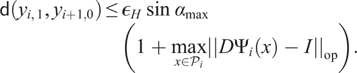
For subsequent charts i, i + 1 traversed by x
π
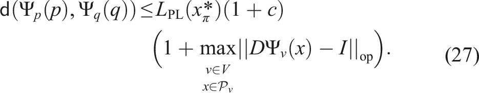
, We now have an upper bound on the error within a chart and across subsequent charts. Thus, by solving the PL-approximation, we obtain an optimal path length
(Approximation Upper Bound)
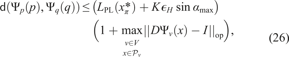
Let Roughly speaking, ϵ
H
sin αmax is a linear approximation of the portion of the path not accounted for within each polytope. If this quantity can be bounded above a multiplicative factor of the portion of the path in each polytope, we can obtain a multiplicative upper bound on
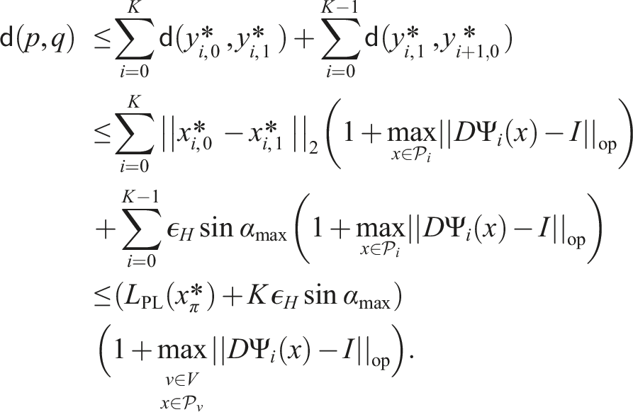
If ∃c > 0 such that
6.5. Planning over SO(3)
The Lie group SO(3) is of great interest in robotics, and thus merits special consideration. For example, the configuration space of a ball joint is a subset of SO(3), and the configuration space of a free moving object in
Let One way to get around this problem is to instead use Euler angles, where a rotation is represented as the product of three rotations, about the x, y, and z axes in a given coordinate system. As a manifold, the set of Euler angles is Another option is to use the approximation strategy described in Subsection 6.4 that can handle arbitrary manifolds, which naturally encompasses SO(3). One can describe SO(3) as the subset of We empirically compare both of these approximations to the Euler angles parametrization in Subsection 7.5. Based on these comparisons, we recommend using the axis-angle parametrization if optimality is a concern, since it can provide a finer approximation than quaternions at a reduced computational cost. If algorithmic runtime is the primary concern, the Euler angles parametrization will lead to the fastest runtimes, but this comes at the cost of suboptimal solutions.
7. Experiments
We demonstrate our GgcsTrajOpt on various robotic platforms. We present illustrative toy examples of planning for a point robot on a toroidal world and an arm in the plane with multiple continuous revolute joints. We also build plans for a KUKA iiwa arm (with the base joint modified to be continuous revolute) and a PR2 bimanual mobile manipulator, implemented in Drake (Tedrake and the Drake Development Team, 2019). We make interactive recordings of these trajectories available online at our results website. For each experiment, we explicitly state the configuration space, using
7.1. Point robot
Consider a point robot moving about a toroidal world (configuration space Results for a point robot in a toroidal world, realized as a unit square with opposite edges identified. Obstacles are shown in red, and each IRIS region is given a distinct pastel color. Note that one of the regions “wraps around” along the horizontal dimension, connecting opposite sides of the world. Grey dashed lines indicate which regions overlap. The optimal path between the start and end points is shown in black.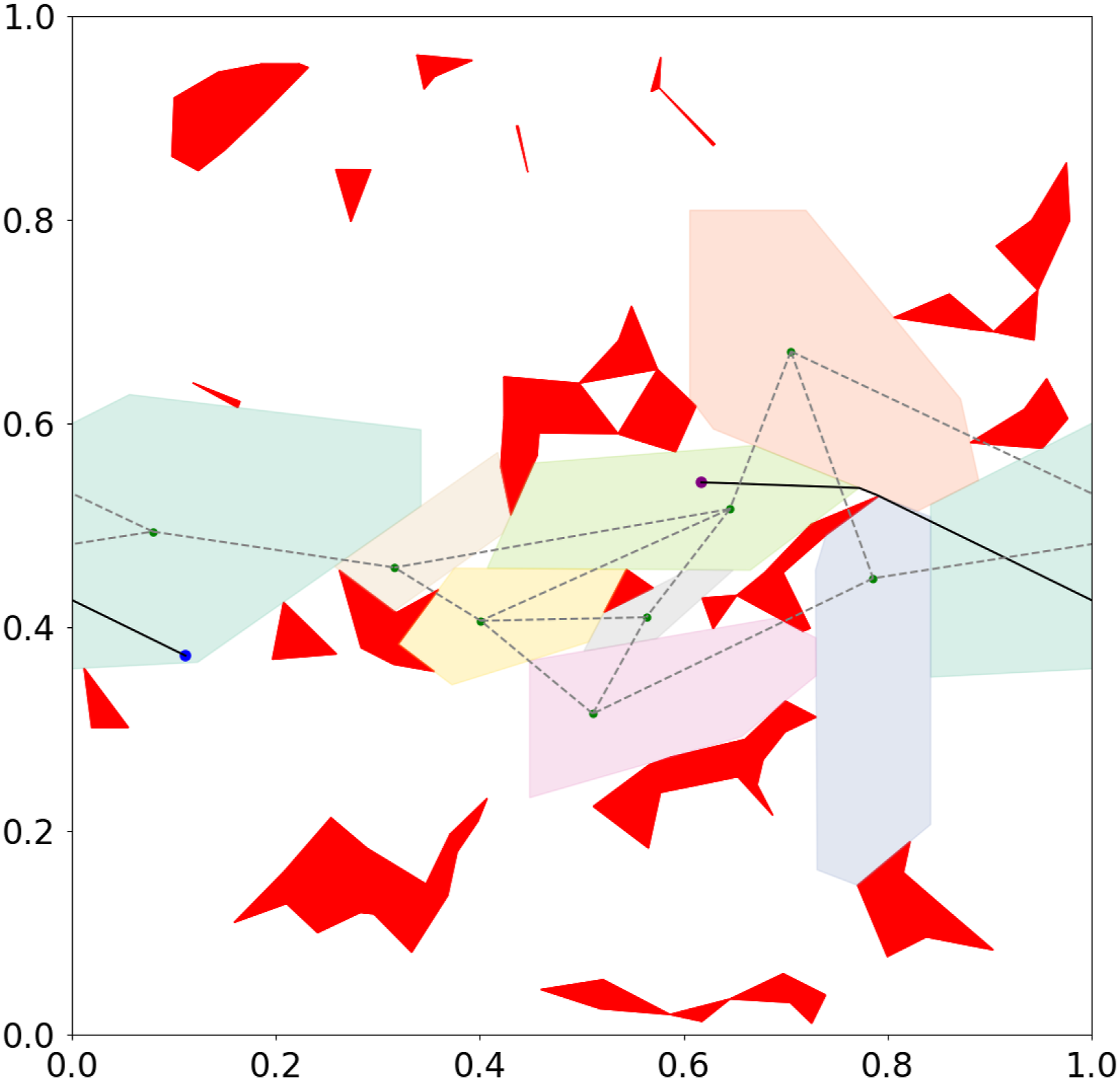
7.2. Planar arm
Consider a robot arm with a fixed base, composed of five continuous revolute joints (configuration space Two plans produced by GgcsTrajOpt for a planar arm around task-space obstacles (shown in red). We display both the swept collision volume and individual poses in the trajectory (colored by time, as indicated by the color bar).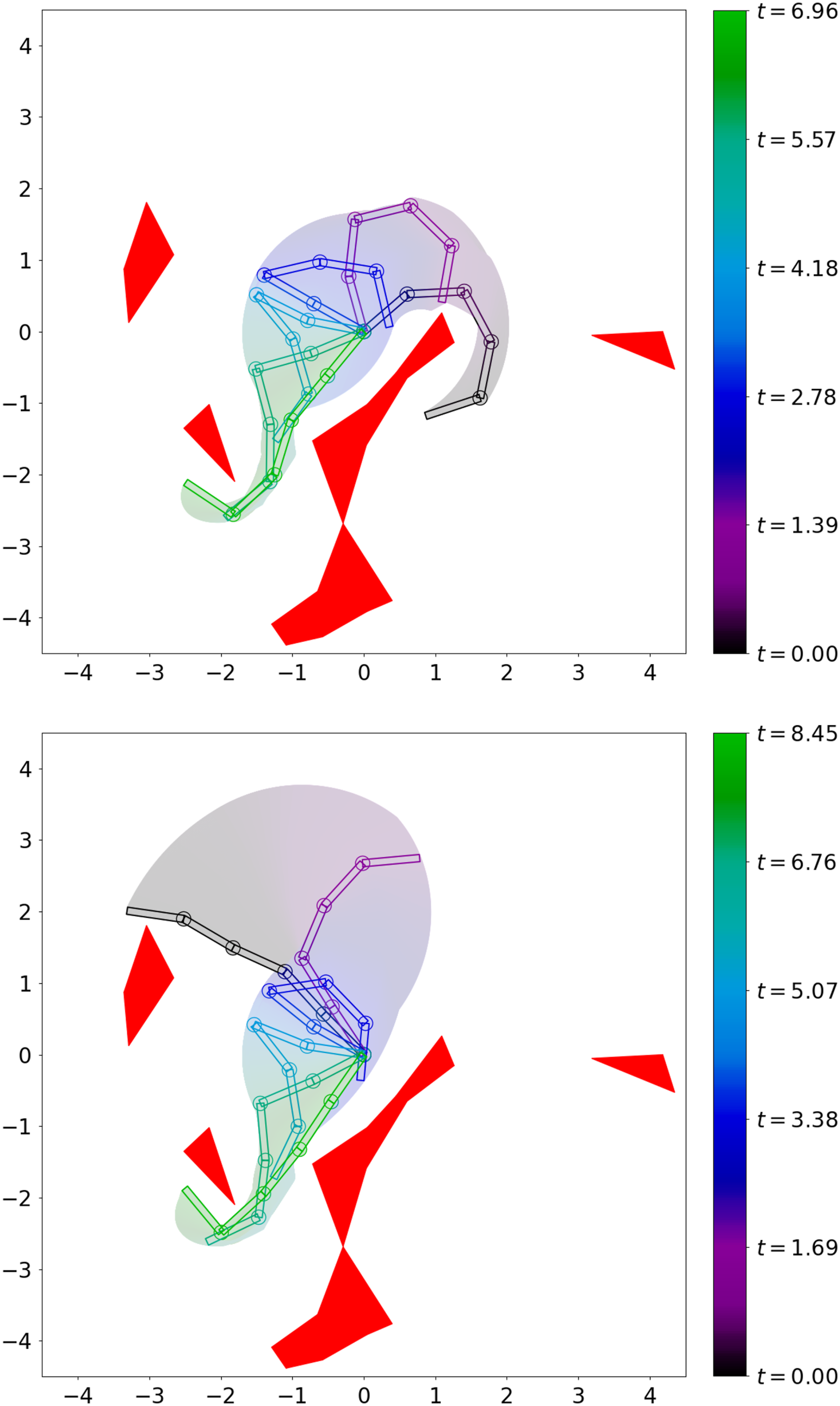
7.3. Modified KUKA iiwa arm
We also demonstrate that GgcsTrajOpt can be used to plan a series of motions using a KUKA iiwa robot arm. The KUKA iiwa is a 7-DoF robot arm where each joint is a revolute joint with limits; in simulation, we remove the limits on the first joint, so the configuration space is
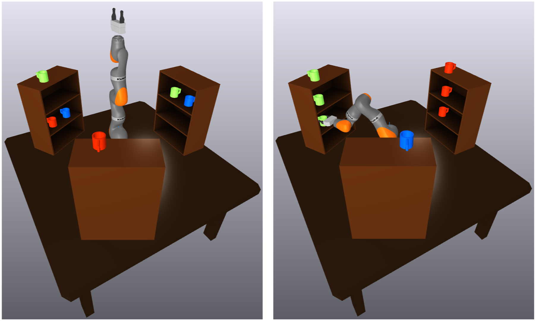
For this experiment, we used a set of 18 convex regions to achieve approximate coverage of the collision-free space. These regions were adjusted as the mugs were moved about the environment and were used to plan the complete motion of the arm—no heuristic motion or “pre-grasp pose” was needed to reach the grasp configuration. Several configurations used to seed the region generation are shown in Figure 7, and the initial and final states are shown in Figure 8. A video and an interactive recording of the plan are available at our results website. Key configurations (overlaid) used for a mug reorganization demo. Initial (left) and final (right) states for the mug reorganization demo.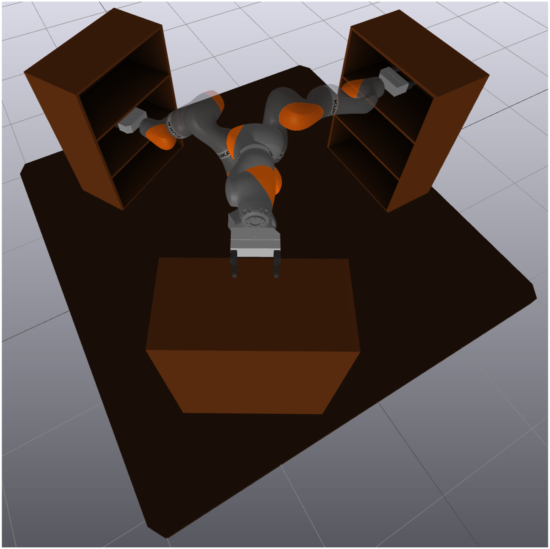
The experiment consisted of 14 motions, which were each planned individually, and we use the region refinement method from Petersen and Tedrake (2023) to account for the current placement of the mugs. This ensured that both the arm and the grasped mug were collision-free for the entirety of each trajectory segment. The robot takes full advantage of the base joint’s lack of limits—always choosing the shortest path and never needing to unwind any rotations. For each segment, planning a trajectory took an average of 25.75 s (with a range of 4.63 to 50.30 s).
7.4. PR2 bimanual mobile manipulator
In addition to its mobile base, the PR2 has two continuous revolute joints in each arm. We have fixed the wrist rotation and gripper joints, so the configuration space is
The performance of GgcsTrajOpt is largely driven by the choice of g-convex sets. For each set of shelves, we generate IRIS regions for the robot to reach into the top, middle, and bottom shelves with both arms simultaneously. We also generate two additional regions where the robot reaches into the middle shelf with one arm and the bottom shelf with the other while crossing its arms. Finally, we manually add various intermediate regions to promote graph connectivity and cover more of C-Free. In Figure 9, we show several robot configurations along a trajectory produced by GgcsTrajOpt. Individual poses along a trajectory produced by GgcsTrajOpt for the PR2 robot, labeled with their order in the plan.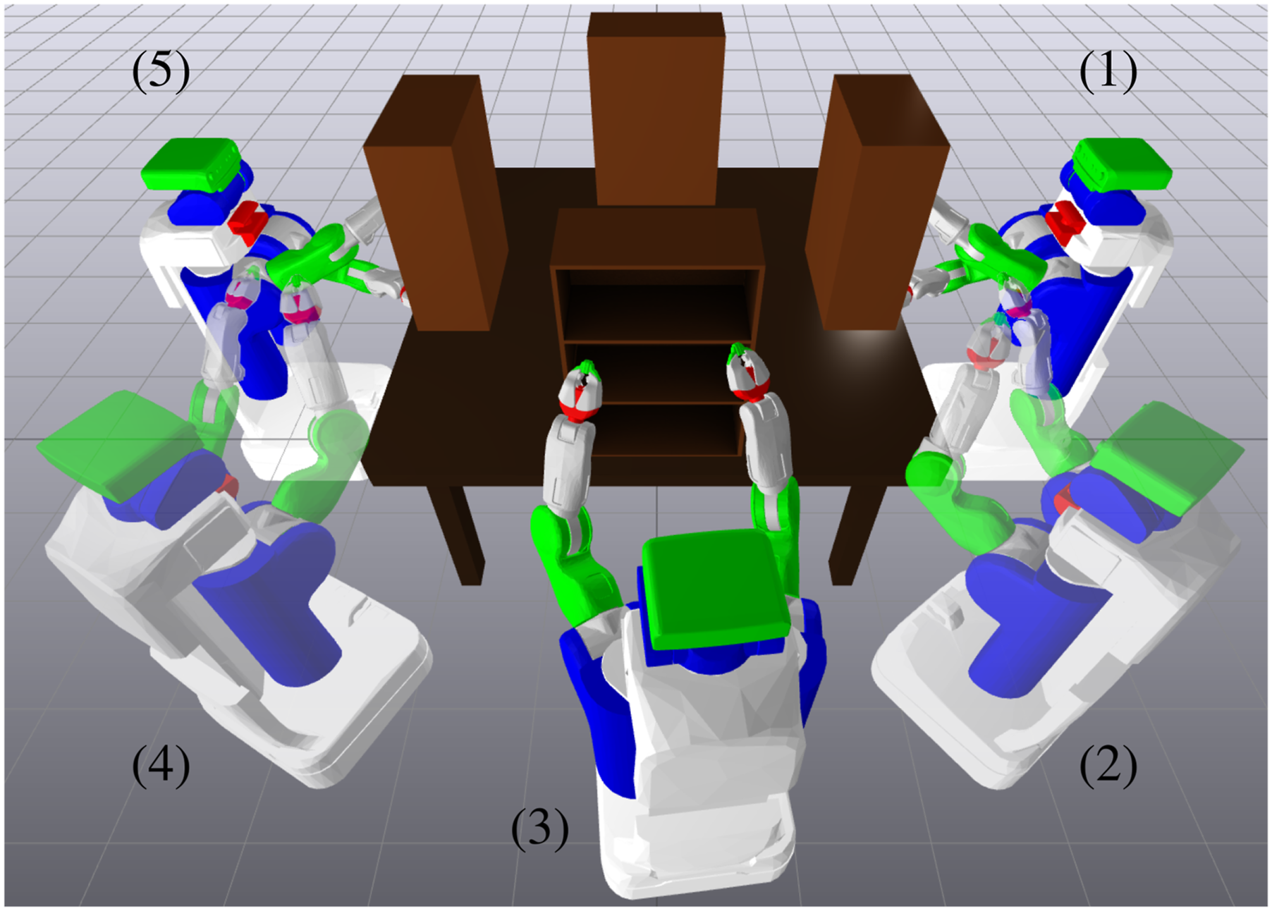
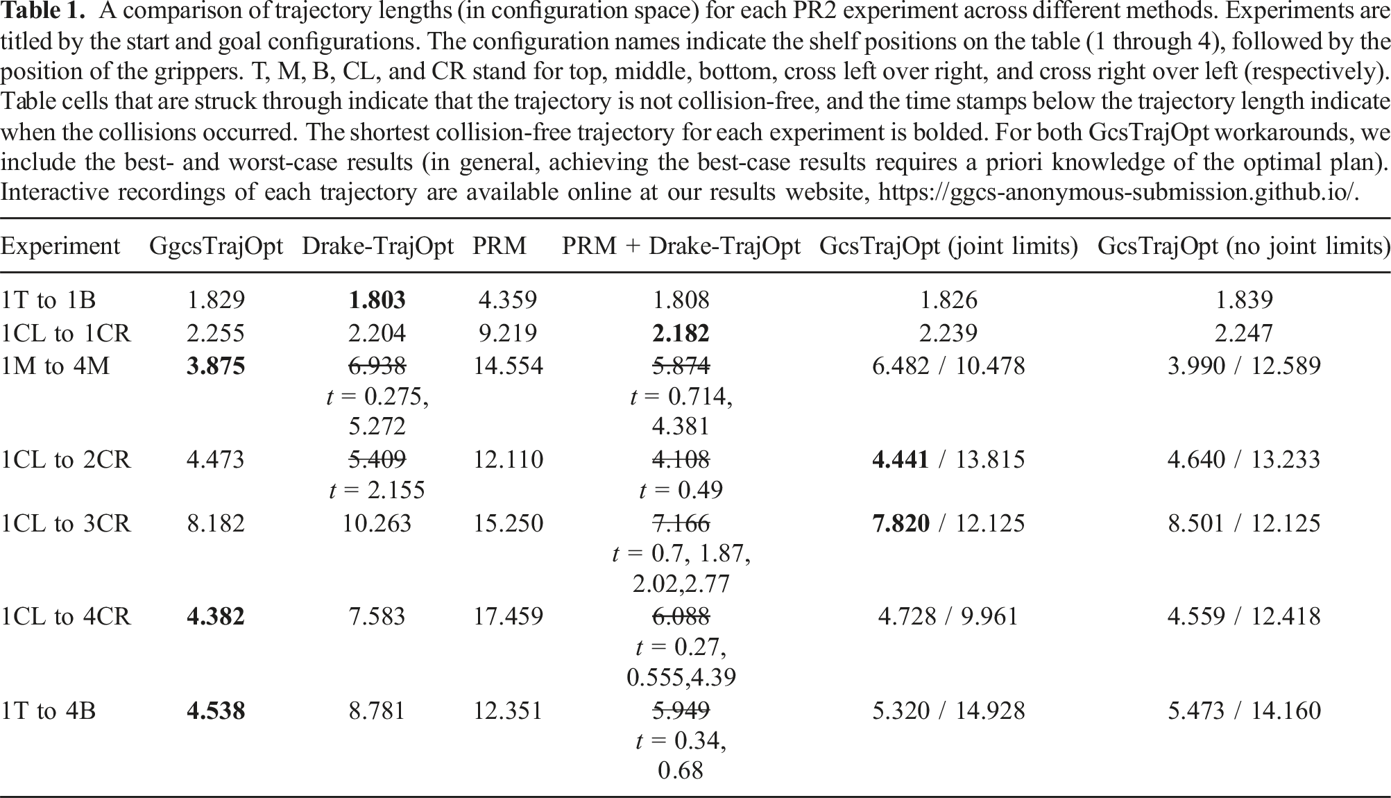
A comparison of trajectory lengths (in configuration space) for each PR2 experiment across different methods. Experiments are titled by the start and goal configurations. The configuration names indicate the shelf positions on the table (1 through 4), followed by the position of the grippers. T, M, B, CL, and CR stand for top, middle, bottom, cross left over right, and cross right over left (respectively). Table cells that are struck through indicate that the trajectory is not collision-free, and the time stamps below the trajectory length indicate when the collisions occurred. The shortest collision-free trajectory for each experiment is bolded. For both GcsTrajOpt workarounds, we include the best- and worst-case results (in general, achieving the best-case results requires a priori knowledge of the optimal plan). Interactive recordings of each trajectory are available online at our results website, https://ggcs-anonymous-submission.github.io/.
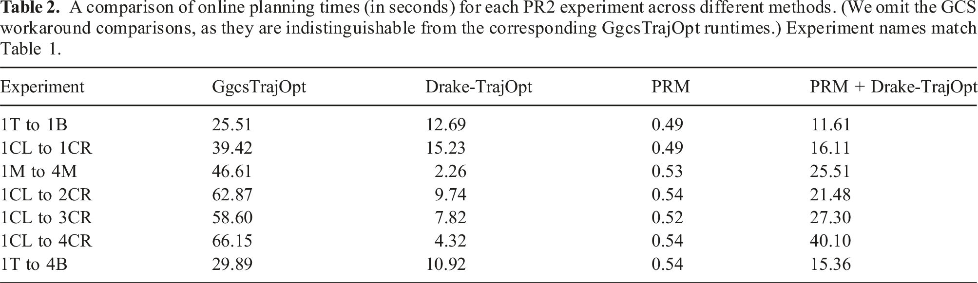
A comparison of online planning times (in seconds) for each PR2 experiment across different methods. (We omit the GCS workaround comparisons, as they are indistinguishable from the corresponding GgcsTrajOpt runtimes.) Experiment names match Table 1.
We also compare it to a sampling-based PRM planner. To mitigate the curse of dimensionality and ensure connectivity between seed points, we initialize the PRM with the skeleton of the GGCS graph: for each pair of overlapping regions, we place a node in the Chebyshev center (Boyd et al., 2004: 148) of their intersection. We then add 100,000 additional samples, drawn uniformly across C-Free (with rejection sampling). This process takes 124.39 s. In comparison, it takes an average of 30.20 s to generate an IRIS region (with a range of 8.56 to 75.42 s). With parallelization, all of the IRIS regions were generated in only 156.63 s.
The plans produced by the PRM are significantly longer than those from the GgcsTrajOpt, so we also examine using the output of the PRM planner as the initial guess for the trajectory optimization. (In principle, this should help prevent Drake-TrajOpt from getting stuck in local minima.) When post-processing PRM plans with Drake-TrajOpt, it sometimes produces shorter final trajectories than GgcsTrajOpt, at the expense of colliding slightly with the environment (an example is shown in Figure 10). This is likely due to the challenge of balancing the collision-free constraint with the minimum distance objective (and because collision-free constraints can only be applied at discrete points). An example of the slight collisions typical of the trajectories produced by Drake-TrajOpt. (The blue circle highlights the point of collision).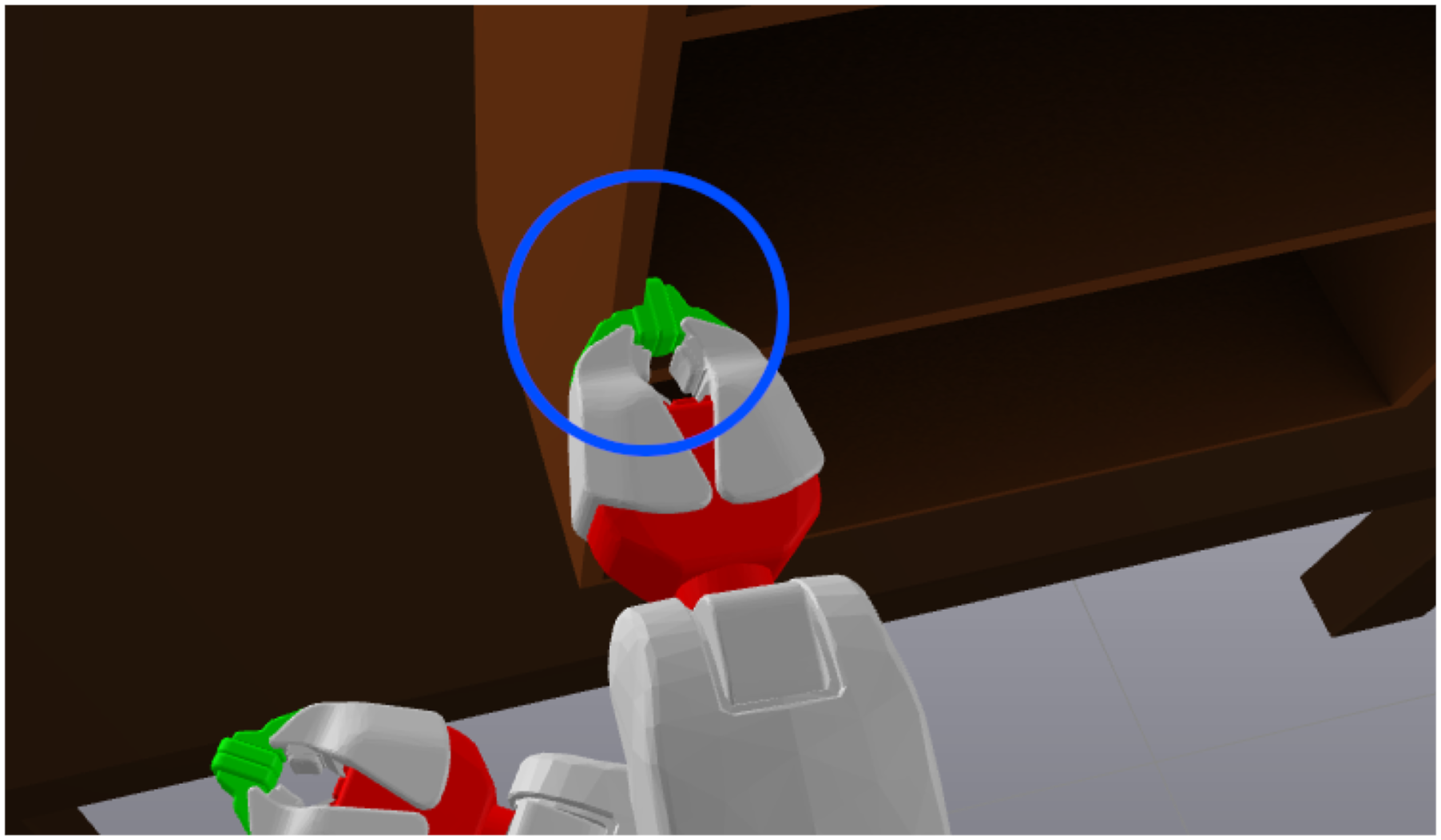
Finally, we compare our GgcsTrajOpt to two workarounds for applying ordinary GCS to non-Euclidean motion planning. One could add artificial joint limits to prevent the wraparound, but placing the joint limits incorrectly could make the optimal path infeasible. The planar arm experiment clearly demonstrates this problem; during the second trajectory in Figure 6, the middle joint traverses more than 360° in the course of the plan. Thus, the optimal trajectory is infeasible for every possible choice of joint limits.
Another option is treating the angles as real numbers with no bound (and ignoring the fact that 0° ≡ 360°). But in this case, the correct joint angle modulo 360° must be chosen to get the optimal path. Furthermore, many copies of each convex set must be made to account for each possible choice of angle modulo 360°, increasing the size of the optimization problem.
With both workarounds, a priori knowledge about the solution is required to guarantee that it is found, so in each comparison, we separately consider the best and worst cases. We use the same seed points across GgcsTrajOpt and both GcsTrajOpt workarounds.
An interesting result is that the best case for the GcsTrajOpt workarounds is sometimes slightly better than GgcsTrajOpt. This is because the sets are not bounded by the convexity radius, so they can grow larger (and cover more of C-Free) with the same seed points. If the workarounds are restricted to using the same regions as GgcsTrajOpt, then, in the best case, their performance is indistinguishable.
7.5. Planning over SO(3)
As discussed in Subsection 6.5, it is necessary to use an approximation strategy to plan over SO(3) with our methodology. To compare the efficacy of the approximation strategies, we consider an abstract planning problem, where we have to find the shortest path (with respect to the canonical bi-invariant Riemannian metric) between two configurations in SO(3). Since there are no obstacles, we can compare the solution from each approximation to the closed-form solution, obtained from spherical linear interpolation (SLERP) (Dam et al., 1998). For numerical purposes, we slightly expand the charts throughout these experiments, so as to achieve a positive-measure overlap.
The Euler angles description is equivalent to
The axis-angle description is equivalent to
The quaternion description is equivalent to
To compare these approximations, we uniformly sampled random start and goal orientations, and computed the shortest path between them for each approximation strategy. We measure their length according to the geodesic distance between each successive control point of the path, and compare to the ground truth distance between the start and goal. Ground truth for this distance metric can be obtained in closed form with spherical linear interpolation (Dam et al., 1998), allowing us to measure the approximation error for each method. In Figure 11, we plot the distribution of the relative errors for each of the three methods. The mean relative errors for each representation are listed in Table 3. The distribution of relative error across many sampled start and goal configurations when planning using various SO (3) approximations strategies. (a) Compared across 1000 random samples, using the lower-resolution approximation of quaternionic sphere. (b) Compared across 250 random samples, using the higher-resolution approximation of quaternionic sphere. A comparison of the mean relative error for each of the four choices of SO (3) representations used with GGCS. All statistics are taken from the experiment with 1000 random samples, except for the high resolution discretization of the quaternion description, which used 250 samples.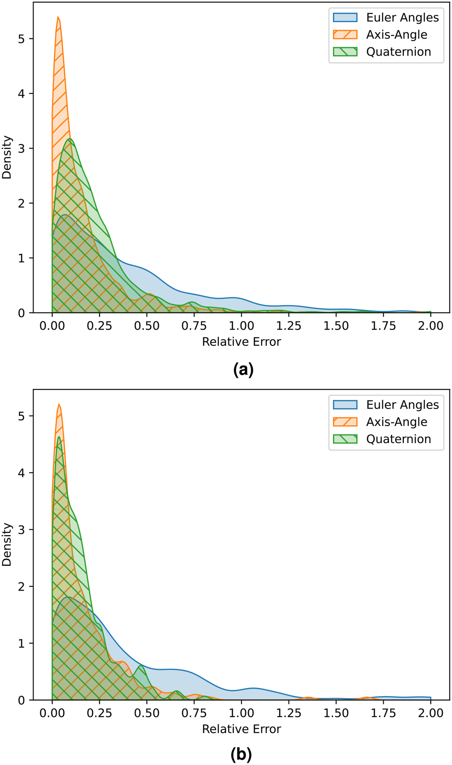
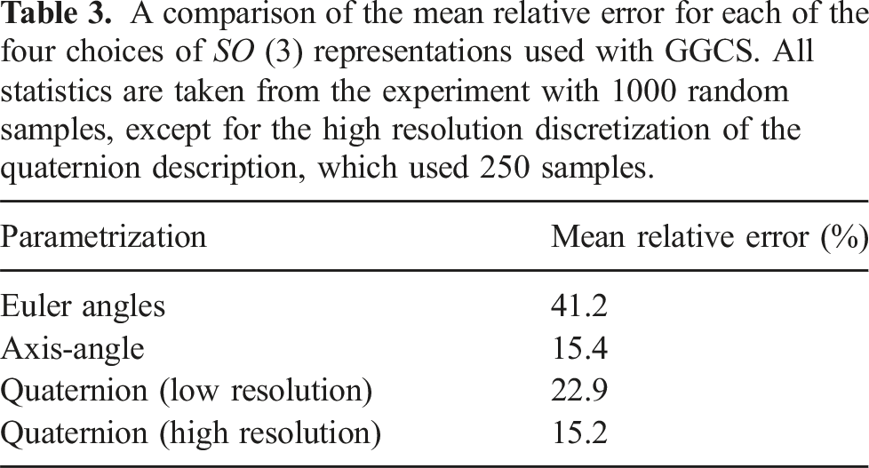
The distance in the Euler angles representation is known to distort the true distance between orientations, so it is unsurprising that this choice of approximation has higher error. If algorithmic runtime is the primary concern, the Euler angles parametrization will lead to the fastest runtimes, but this comes at the cost of suboptimal solutions. When the higher-resolution approximation of the quaternionic sphere is used, its relative error is roughly equivalent to that of the axis-angle approximation. However, this requires a much larger graph (and many more edges), yielding a more computationally costly optimization program. Thus, we recommend using the axis-angle parametrization, as it strikes the best balance between accuracy and computational efficiency.
7.6. Planning over SE(3)
In this experiment, we use GgcsTrajOpt to produce plans for a block moving freely throughout a maze. The maze has a 2D layout, similar to the maze shown in Figure 2 of (Marcucci et al., 2023), but the walls of the maze enclose a 3D world. The block is allowed to move freely through the maze—its configuration space is SE(3). However, it is not allowed to leave the maze along the vertical direction; the center of the block is constrained to lie between the top and bottom of the maze walls. We produce plans between nine different key poses of the block, shown within the maze in Figure 12. Above each of these poses, the orientation of the block is annotated with a coordinate frame. These various orientations differ by rotations of up to 180° along all three axes. Thus the planner must carefully reason about which way the block should rotate around any given axis over the course of the trajectory. The maze environment used for an SE (3) planning problem. The block is allowed to move freely within the maze, including arbitrary rotations and translations in 3D space. The nine configurations shown have various orientations, which are indicated by the coordinate frames superimposed above each configuration. Note that some of these orientations include requiring a complete flip of 180° about a horizontal axis (e.g., between the top-right and top-center configurations).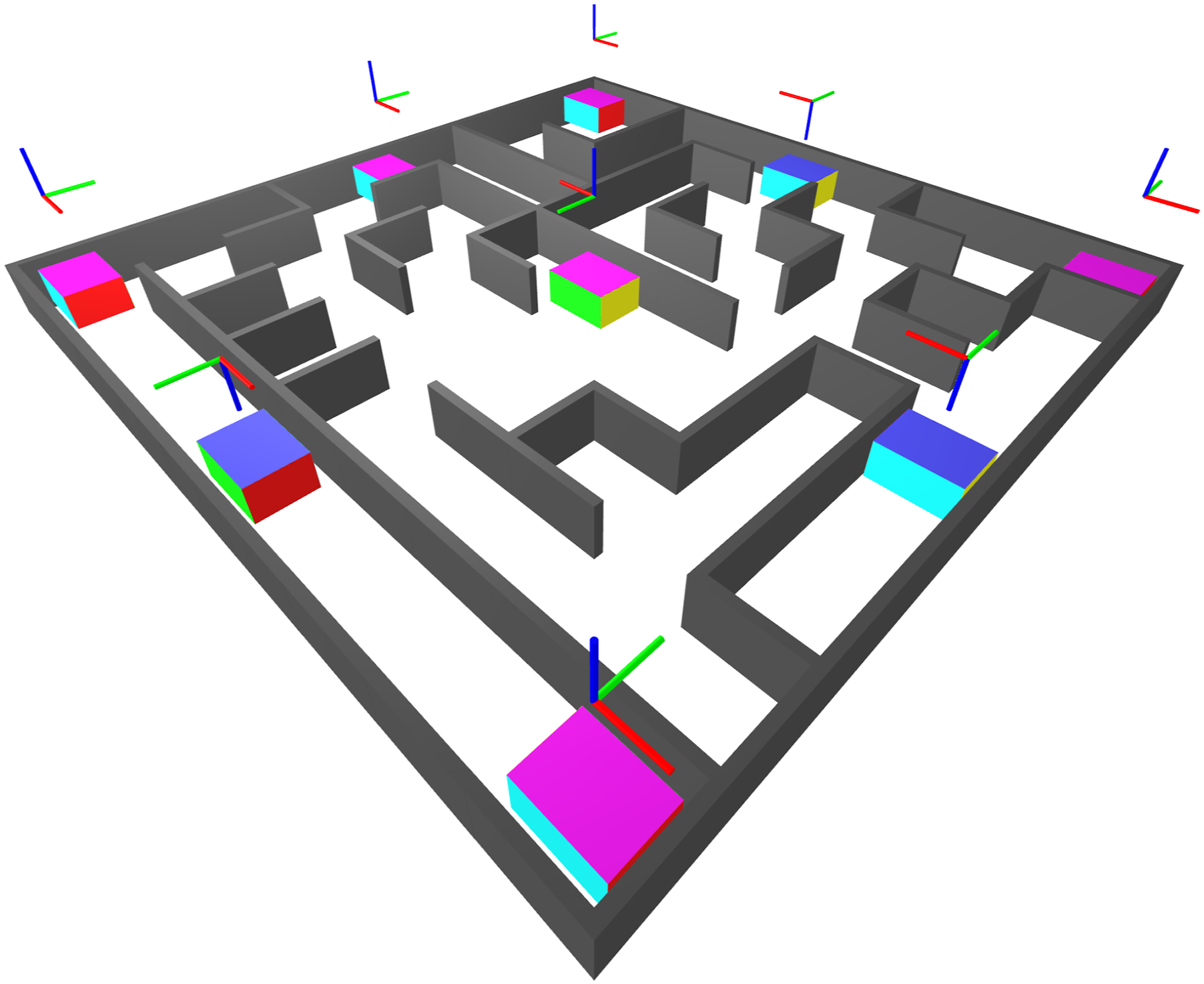
We use Euler angles in our representation of SE(3) because we do not yet know how to get collision free regions with PL approximations. We treat the three Euler angles as if they are three successive continuous revolute joints. So we allow the regions to grow up to π − ϵ in diameter along each revolute axis. We construct a coarse grid roadmap of the maze and grow regions to cover a subset of the edges so as to connect the key poses. This results in a GGCS with 200 sets and 4744 (directed) edges. The polytopes were described by an average of 26.095 halfspaces (minimum 21, maximum 35) and took 65.434 s to compute (without leveraging any parallelization).
Given this GGCS, we solve the shortest path problem for every choice of start and goal. Due to the large size of this problem instance, the memory and runtime requirements to solve the convex relaxation are prohibitive. As a mitigation strategy, we replace the 2-norm in the objective of (20) with the 1-norm when solving the convex relaxation. This yields a linear program, which can be solved much more efficiently than the second-order cone program that would result from the 2-norm objective. We observe that in this problem instance, the objective functions are similar enough that we can still use the downstream rounding process to produce high-quality trajectories. We still use the original 2-norm objective to minimize path length in the rounding stage. This can be seen as an instance of the technique, introduced in von Wrangel (2024), of using different costs and constraints for the relaxation and rounding stages.
We also use relatively loose tolerances when solving the relaxation to further improve runtimes. (In particular, we use 10−3 as the termination tolerance for primal feasibility, dual feasibility, and relative gap.) This is acceptable because the downstream rounding process is robust to such inaccuracies; the flows are known to only heuristically indicate the shortest path, even when the convex relaxation is solved to an arbitrarily tight numerical tolerance. In the rounding stage, each individual optimization problem is much smaller, so we can use a tight tolerance to ensure constraints on the trajectory are properly enforced. The average solve time with this approach was 354.98 s, and we visualize a planned trajectory in Figure 13. Solution path for a planning problem in the maze environment. Paths were obtained with the relax-and-round strategy.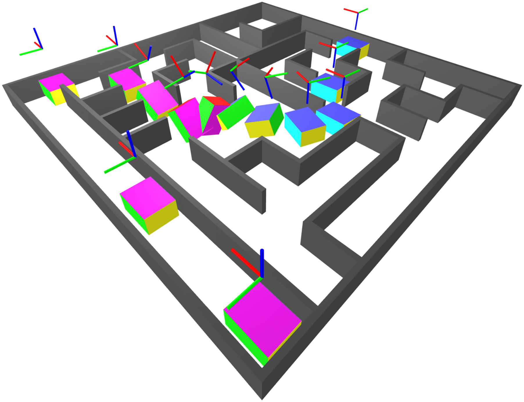
An alternative approach to solving GCS problems with excessively large graphs is the GCS* algorithm (Chew Chia et al., 2024). GCS* solves a shortest path problem on a GCS using graph search techniques, similar to the famous A* search algorithm (Hart et al., 1968). The average solve time with GCS* was only 46.71 s—13.5% of the runtime of the relax-and-round solution method. And the paths produced by GCS* were only 4.4% longer than those found with the relax-and-round strategy.
8. Discussion
In this paper, we have formulated the general problem of motion planning around obstacles on Riemannian manifolds as a shortest path problem in a graph of geodesically convex sets, and we have presented sufficient conditions under which this formulation inherits the same guarantees as in the ordinary Euclidean case. We describe how these theoretical developments inform simple and elegant modifications to the original GcsTrajOpt, in order to handle robots with mobile bases and continuous revolute joints. This enables us to solve motion planning problems on such robotic platforms to global optimality and guarantee that the trajectory is collision-free at every point in time. Approximate solving techniques still guarantee that trajectories are collision-free, and empirically, such trajectories are very close to optimal.
The PL approximation strategy has the benefit of being applicable to arbitrary manifolds, and can produce arbitrarily fine approximations given sufficient computation time. However, it remains to be seen whether that runtime will become prohibitive if this strategy is used for more complex robot configuration spaces. The use of heuristic strategies to handle large problems, such as GCS* (Chew Chia et al., 2024) is a promising direction for keeping computational costs low even as the problems grow in complexity. Another limitation of the PL approximation strategy is the lack of a general approach for producing collision-free regions. For now, we must rely on workarounds such as flat parametrizations and accept the resulting distortion of the objective function.
We have demonstrated that GgcsTrajOpt is a powerful tool for robot motion planning. It is capable of producing plans for high degree-of-freedom systems operating in obstacle-dense configuration spaces, such as a PR2 bimanual mobile manipulator reaching into and out of shelves. Although the planning and optimization frameworks used in GgcsTrajOpt are still in their infancy, they are already capable of producing high-quality results that are competitive with existing methods. As further research and technical improvements are made, its performance will continue to improve.
Footnotes
Acknowledgements
The authors would like to thank Tobia Marcucci and Seiji Shaw for their valuable suggestions throughout the course of this work. The authors would also like to thank David von Wrangel for his assistance with the implementation of the PRM comparisons and Shao Yuan Chew Chia for applying the GCS* algorithm to our problem domain.
Declaration of conflicting interests
The author(s) declared no potential conflicts of interest with respect to the research, authorship, and/or publication of this article.
Funding
The author(s) disclosed receipt of the following financial support for the research, authorship, and/or publication of this article: This work was supported by (in alphabetical order) Amazon.com, PO No. 2D-06310236 and the Frederick and Barbara Cronin Fellowship.