
Abstract
We present novel, convex relaxations for rotation and pose estimation problems that can a posteriori guarantee global optimality for practical measurement noise levels. Some such relaxations exist in the literature for specific problem setups that assume the matrix von Mises-Fisher distribution (a.k.a., matrix Langevin distribution or chordal distance) for isotropic rotational uncertainty. However, another common way to represent uncertainty for rotations and poses is to define anisotropic noise in the associated Lie algebra. Starting from a noise model based on the Cayley map, we define our estimation problems, convert them to Quadratically Constrained Quadratic Programs (QCQPs), then relax them to Semidefinite Programs (SDPs), which can be solved using standard interior-point optimization methods; global optimality follows from Lagrangian strong duality. We first show how to carry out basic rotation and pose averaging. We then turn to the more complex problem of trajectory estimation, which involves many pose variables with both individual and inter-pose measurements (or motion priors). Our contribution is to formulate SDP relaxations for all these problems based on the Cayley map (including the identification of redundant constraints) and to show them working in practical settings. We hope our results can add to the catalogue of useful estimation problems whose solutions can be a posteriori guaranteed to be globally optimal.
Keywords
1. Introduction
State estimation is concerned with fusing several noisy measurements (and possibly a prior model) into a less noisy estimate of the state (e.g., position, velocity, orientation) of a vehicle, robot, or other object of interest. Real-world state estimation problems often involve measurement functions and motion models that are nonlinear with respect to the state. Alternatively, the state itself may not be an element of a vector space, such as the rotation of a rigid body. These challenging aspects typically mean that when we set up our estimator as an optimization, it is a nonconvex problem; the cost function, the feasible set, or both are not convex. Nonconvex optimization problems are in general much harder to solve than convex ones because they can have local minima and common gradient-based optimizers can easily become trapped therein.
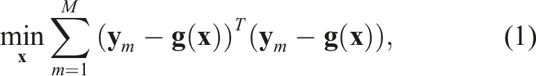
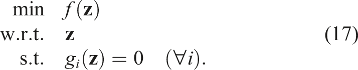
For example, we might have a generic nonlinear least-squares problem such as
There has been quite a bit of work in robotics and computer vision aimed at the idea of solving estimation problems globally. Most of these works employ sophisticated tools from the optimization literature to achieve this. In particular, Lagrangian duality is used to derive convex relaxations, which can be solved globally. Boyd and Vandenberghe (2004, §5) provide the necessary background on duality theory. We will be following a common pathway where we first convert our nonconvex optimization problem into another nonconvex form called a Quadratically Constrained Quadratic Program (QCQP); from here we relax this to a (convex) Semi-definite Program (SDP), amenable to off-the-shelf solvers (e.g., the interior-point-based SDP solver in
As mentioned, the convex relaxation procedure we employ has been well known in the optimization community for some time. In particular, it has been used for polynomial optimization (Parrilo, 2003) and in various combinatorial optimization problems, such as quadratic assignment (Nesterov et al., 2000) and max-cut graph partitioning (Anjos and Wolkowicz, 2002). To the authors’ knowledge, the first use of SDP relaxations in the robotics community was by Liu et al. (2012) for planar Simultaneous Localization and Mapping (SLAM), though their application in computer vision (Kahl and Henrion, 2005) and signal processing (Krislock and Wolkowicz, 2010; Luo et al., 2010) occurred earlier. More generally, Cifuentes et al. (2022) provides a nice overview of some common problems in computer vision and robotics where these tools have been applied before, as well as providing a rationale for why they are so effective. One of the most commonly investigated relaxations in the robotics and vision communities is rotation synchronization 1 (Bandeira et al., 2017; Dellaert et al., 2020; Eriksson et al., 2018, 2021); here several rotations are linked through noisy relative rotation measurements. Rotation synchronization turns out to be the nucleus of several of the other problems under study including pose-graph optimization (Briales and Gonzalez-Jimenez, 2017a; Carlone and Calafiore, 2018; Carlone et al., 2016; Rosen et al., 2019; Tian et al., 2021), point-set registration (Chaudhury et al., 2015; Iglesias et al., 2020; Yang et al., 2021), calibration (Giamou et al., 2019; Wise et al., 2020), mutual localization (Wang et al., 2022b), and landmark-based SLAM (Holmes and Barfoot, 2023). Rotation synchronization and its cousins have been shown to admit fast solutions through low-rank factorizations (Rosen et al., 2019). More recently, other measurement models such as range sensing have also been incorporated into globally certifiable problems (Dümbgen et al., 2023; Papalia et al., 2023).
It is worth also mentioning the works of Forbes and De Ruiter (2015); Horowitz et al. (2014) on globally optimal pointcloud alignment, which also employ convex relaxation, but the route to the SDP is not Shor’s relaxation; instead, Lie group optimization variables are relaxed to live in a convex set. On the surface, this approach is not applicable to the problems considered herein; for example, our cost functions are not always initially convex.
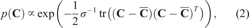
A common thread that ties most of the existing literature together is that the chordal distance is used to construct the terms of the cost function that involve rotation variables. Viewed through a probabilistic lens, the chordal distance is related to the matrix Langevin or matrix von Mises-Fisher distribution, whose density can be written in the form
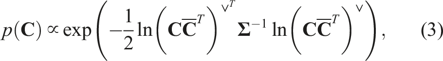
To our knowledge, the examination of global optimality for state estimation problems where rotational (and pose) uncertainty is defined in this way has not be explored previously in the literature. Our novel contribution is therefore a family of specific convex relaxations of rotation and pose estimation problems formulated using the Cayley map (including redundant constraints needed to make them work in practice); this is important as it opens the door to providing certification for a broad class of state estimation problems used in practice.
This paper is organized as follows. In Section 2, we review the relevant mathematical background including Lie groups, the Cayley map, and the convex relaxation procedure that we will employ. Section 3 presents the basic problems of averaging a number of noisy rotation or pose measurements. In Section 4, we expand the method to include discrete-time trajectory estimation of several poses based on individual and inter-pose measurements. Section 5 expands this to include so-called continuous-time trajectory estimation where we have a smoothing assumption on the trajectory and estimate both pose and twist at each state. In each of Sections 3 to 5, we provide experimental results that demonstrate the viability of our convex relaxations to find globally optimal solutions. Section 6 concludes the paper. Appendix A discusses the similarity between distributions defined using the exponential and Cayley maps while Appendix B presents the baseline local solvers to which we compare our new global estimates.
2. Mathematical background
We begin by reviewing the relevant background concepts for the paper including Lie groups, the Cayley map, and convex relaxations of nonconvex optimization problems via Lagrangian duality.
2.1. Lie groups for rotations and poses
The special orthogonal group, representing rotations, is the set of valid rotation matrices:


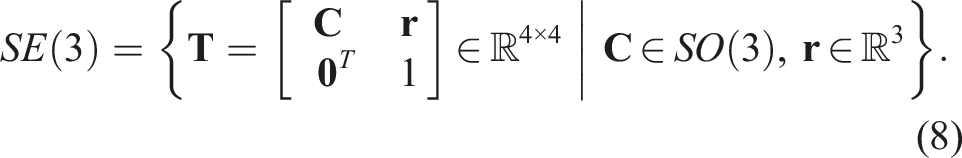
The special Euclidean group, representing poses (i.e., translation and rotation), is the set of valid transformation matrices:
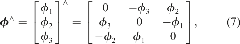
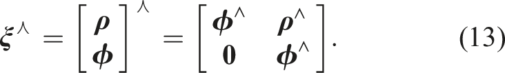
It is again common to map a vector,

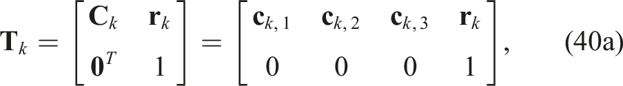
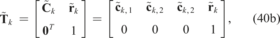
where we have overloaded the ∧ operator as
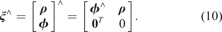
Notationally, we will use ∨ to mean the inverse operation of ∧. As is common practice (Barfoot, 2024), we have broken the pose vector,
Finally, the adjoint of a pose is given by
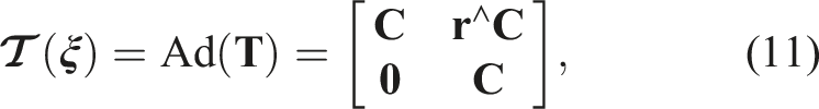
which is now 6 × 6. We will refer to the set of adjoints as Ad(SE(3)). We can map a vector,

2.2. Cayley map
While the exponential map is the canonical way to map from a Lie algebra (vector space) to a Lie group, it is not the only possibility. There are in fact infinitely many such vectorial mappings for SO(3) (Bauchau and Trainelli, 2003), SE(3) (Barfoot et al., 2022), and Ad(SE(3)) (Bauchau, 2011; Bauchau and Choi, 2003).
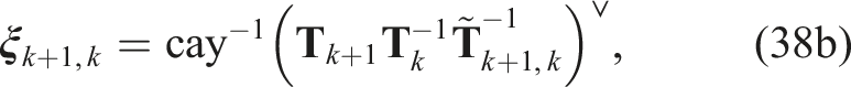
In particular, it is well known that for the Cayley-Gibbs-Rodrigues parameterization of rotation we can write the rotation matrix in terms of the Cayley map,
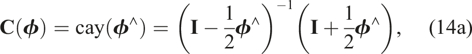

for some
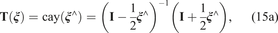

for some
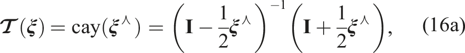

However, Selig (2007) demonstrates that starting from the same
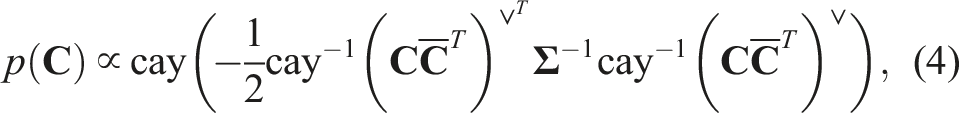
Figure 1 provides examples comparing two rotational distributions derived from the exponential and Cayley maps that have approximately the same variance; we can see that even with quite large rotational uncertainty they match quite closely. Appendix A provides some further discussion on how closely these distributions can be made to match. The key idea of the paper will be to replace instances of the exponential map with the Cayley map, which we will see is more amenable to producing polynomial optimization problems, a key prerequisite to our route to global optimality. Comparison of uncertainty on rotation angle, φ, for the exponential and Cayley maps, where the variances have been approximately matched (see Appendix A for further discussion of how this was done). (left) Standard deviation of rotational uncertainty is σ = 0.2 [rad]. (right) σ = 0.5 [rad]. The match is good in both cases with more divergence as rotational uncertainty increases.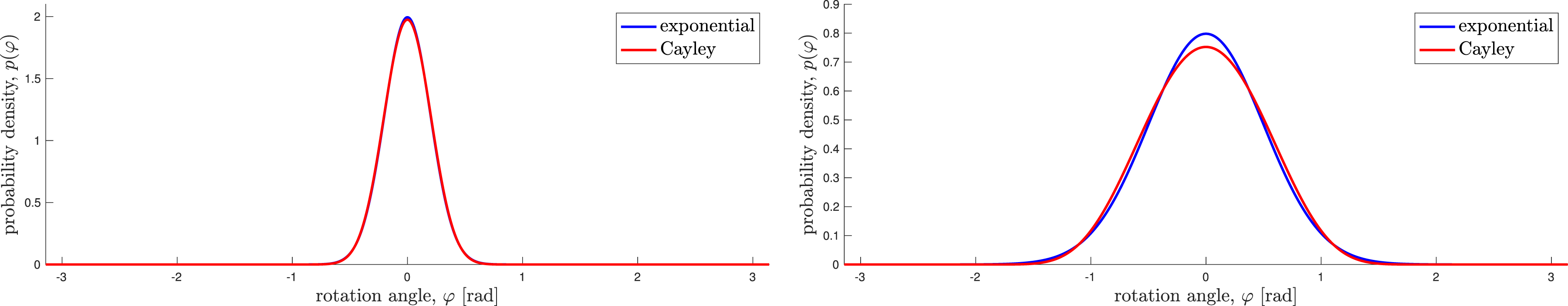
The Cayley map has been used in the past for rotation, pose, and trajectory estimation (Alismail et al., 2014; Barfoot et al., 2022; Junkins et al., 2011; Majji et al., 2011; Mortari et al., 2007; Qian et al., 2020; Wong et al., 2018; Wong and Majji, 2016), typically to parameterize rotations or poses thereby creating a simpler unconstrained quadratic optimization problem. The drawback of these approaches is that they are still subject to singularities and local minima. The Cayley map has also been used to achieve global optimality in the perspective-n-point (PnP) problem (Nakano, 2015; Wang et al., 2022a); we take a quite different approach, however, through the use of convex relaxations. Additionally, the Cayley map has found application in parametrizing lines in structure from motion, as an unconstrained alternative to parametrizations such as Plücker coordinates (Zhang and Koch, 2014).
The Cayley map has also been employed in areas of robotics other than estimation. In Kobilarov (2014); Kobilarov and Marsden (2011), for example, the authors suggest using the Cayley map for rotation parametrization in the context of optimal control of mechanical systems on Lie groups. The authors observe that, compared with the exponential map, the Cayley map is computationally more efficient because of its simpler structure, in particular as it circumvents trigonometric functions. It is also noted that the Cayley map has no singularities in its gradients, which is of advantage for the numerical stability of commonly used solvers (Kobilarov and Marsden, 2011). In Solo and Wang (2019), the Cayley map is employed for simulating stochastic differential equations that evolve on Stiefel manifolds, which is subsequently used in Wang and Solo (2020) for a novel particle filter variant. It is possible that our global optimality approach to using the Cayley map could be employed within some of these applications, but we leave this investigation for future work.
2.3. Convex relaxations
We next summarize the key optimization tools that we will use. Boyd and Vandenberghe (2004) provide the appropriate background. Suppose that we have a nonconvex optimization problem of the form
We attempt to introduce appropriate nonlinear substitution variables,
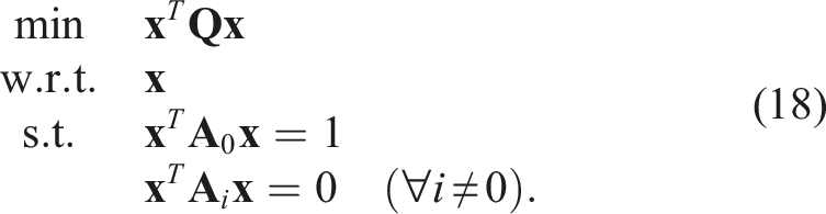
This problem is a Quadratically Constrained Quadratic Program (QCQP), which is still nonconvex and typically of higher dimension than the original problem, but possesses more exploitable structure. Next, by defining
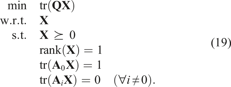
Finally, if we drop the rank(
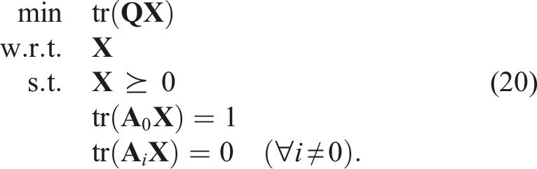
This is known as Shor’s relaxation (Shor, 1987). If the solution to this problem happens to result in rank(
Unfortunately, for most problems in this paper, Shor’s relaxation is not tight out of the box. In this paper, tightness means rank(
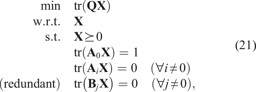
The technique of adding redundant constraints to improve the tightness of a given SDP relaxation has been known for some time in the optimization literature (Anstreicher and Wolkowicz, 2000; Nesterov et al., 2000). More recently, there have been several cases in which redundant constraints have been used in the robotics (Yang et al., 2021; Yang and Carlone, 2023; Giamou et al., 2019; Wang et al., 2022b) and machine vision (Briales et al., 2018; Briales and Gonzalez-Jimenez, 2017b; Garcia-Salguero et al., 2022; Kezurer et al., 2015) literature. With redundant constraints, our problem becomes
3. Averaging
We will build up our optimization problems gradually starting with simply ‘averaging’ several noisy estimates of rotation or pose.
3.1. Rotation averaging
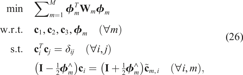
In order to average M rotations, we could set up an optimization problem as
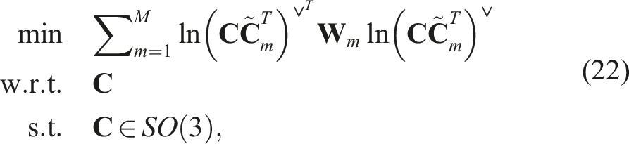

This is where the main insight of the paper comes in. We can substitute the Cayley map for the exponential map without too much effect on the stated problem (see Figure 1). With this substitution, our generative model for noisy rotations becomes

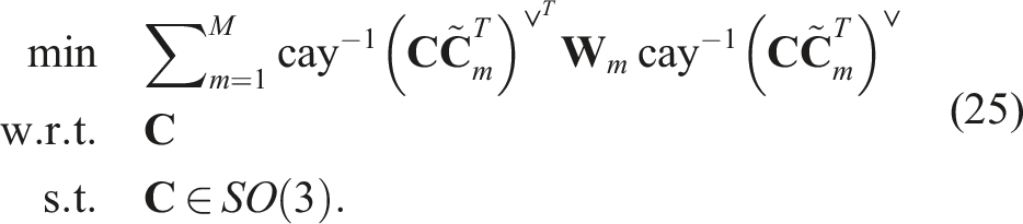
Now our cost represents the negative log-likelihood of the joint distribution of the measurements, assuming each obeys (4). Turning this into a QCQP is then fairly easy:

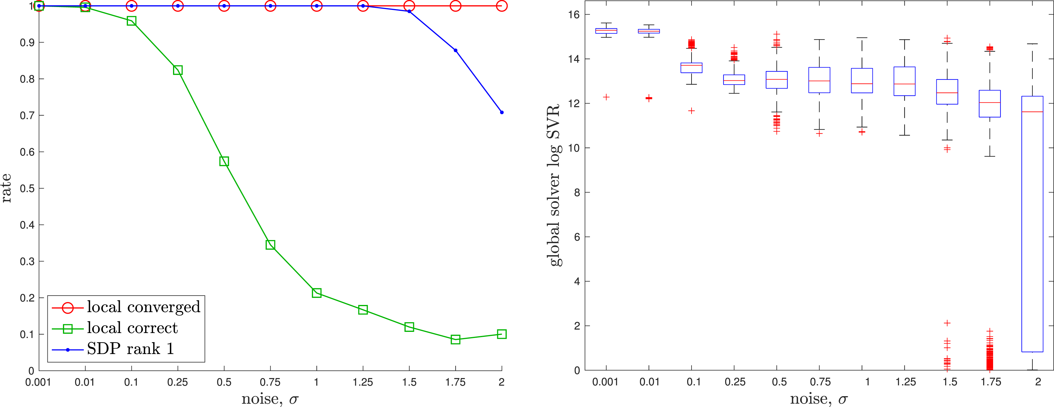
The details of a baseline local solver can be found in the appendix. For the global (SDP) solver we used Rotation Averaging: An example of noisy rotation averaging where the randomly initialized local solver (dotted) becomes trapped in a poor local minimum while the global solver (dashed) finds the correct global solution, which is closer to the groundtruth rotation (solid). Rotation Averaging: A quantitative evaluation of the tightness of the rotation averaging problem with increasing measurement noise level, σ. At each noise level, we conducted 1000 trials of averaging 10 noisy rotations. (left) We see that the local solver (randomly initialized) finds the global minimum with decreasing frequency (green) as the measurement noise is increased, while the SDP solver (blue) successfully produces rank-1 solutions (we consider log SVR of at least 5 to be rank 1) to much higher noise levels. For completeness, we also show how frequently the local solver converges to any minimum (red). (right) Boxplots of the log SVR of the SDP solution show that the global solution remains highly rank 1 over a wide range of measurement noise values.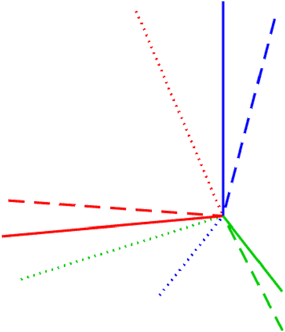
3.2. Pose averaging
Pose averaging follows a very similar approach to the previous section.
4
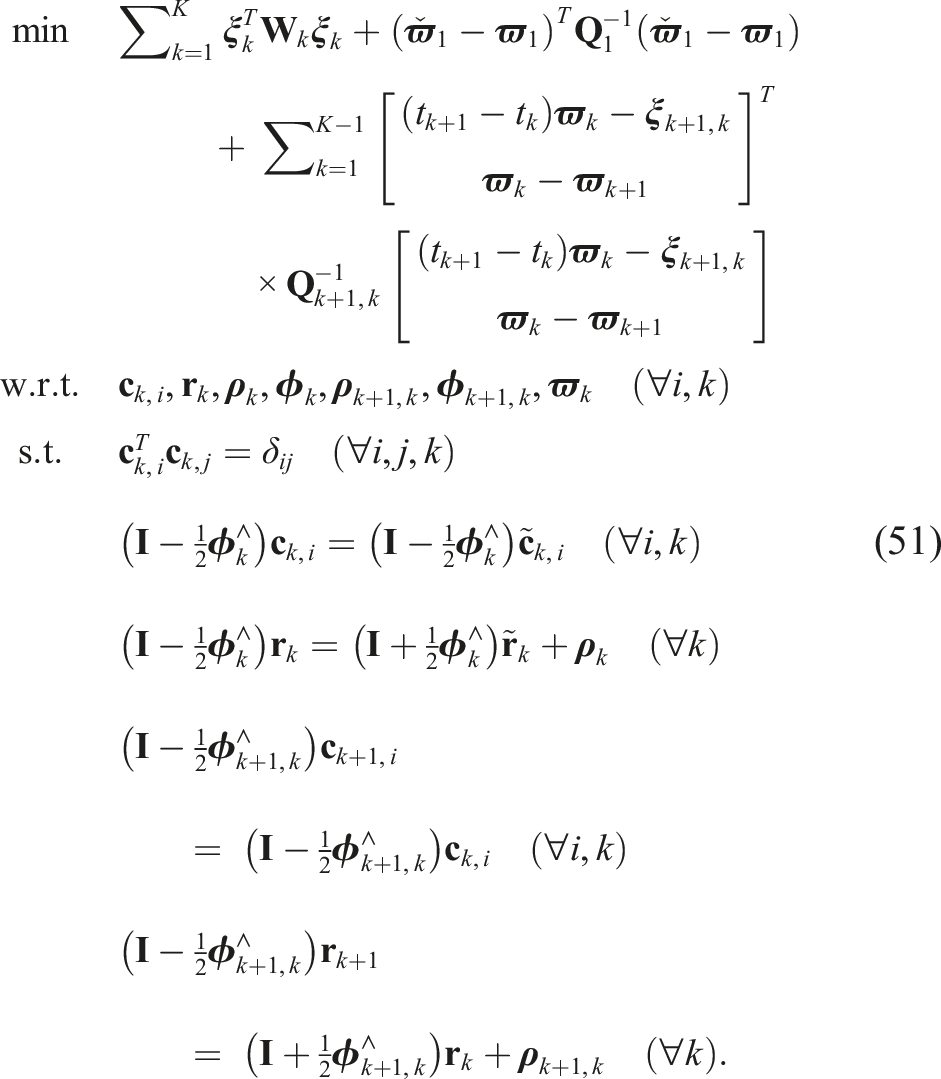
An optimization problem based on the Cayley map can be stated as
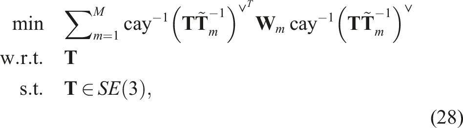
We convert the residual pose errors,
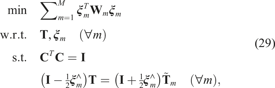
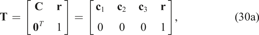
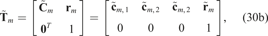
and then rewrite the optimization problem using the reduced set of variables as
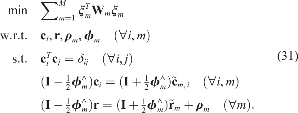
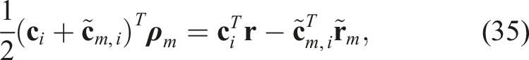
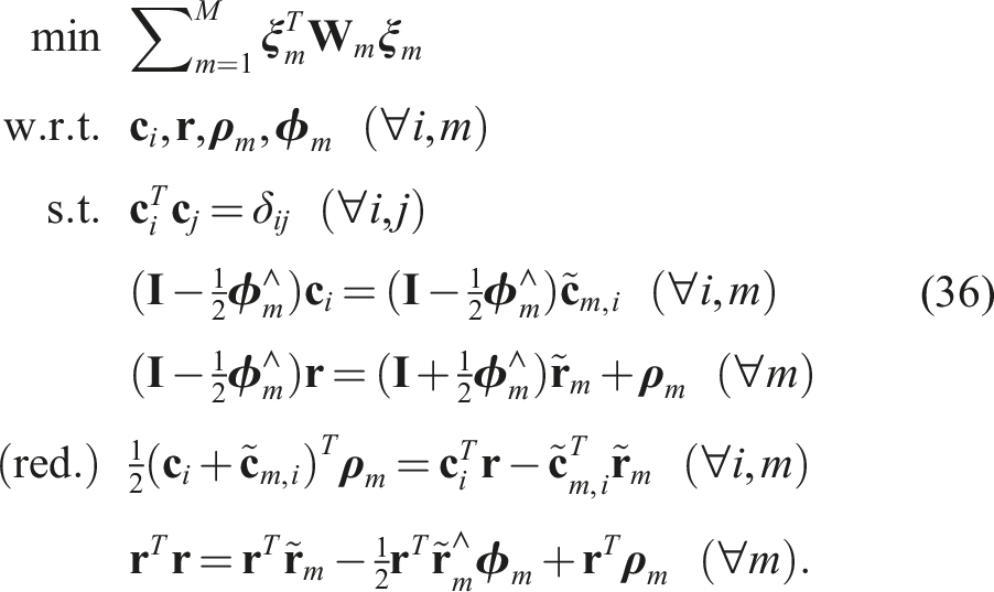
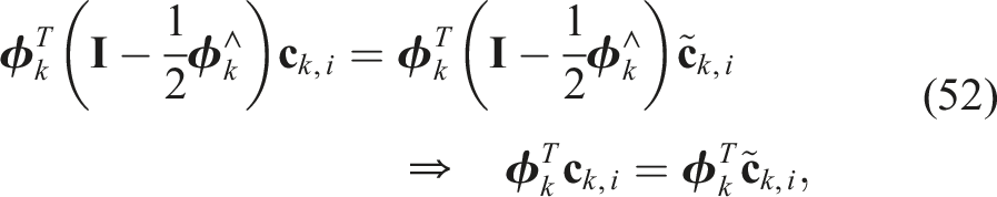
This is now a QCQP, but unfortunately when we relax to a SDP, it is not always tight even for low-noise levels. We found that introducing specific redundant constraints for each m tightens the problem nicely for practical noise levels. One such useful constraint can be found by premultiplying the last constraint in (31) by
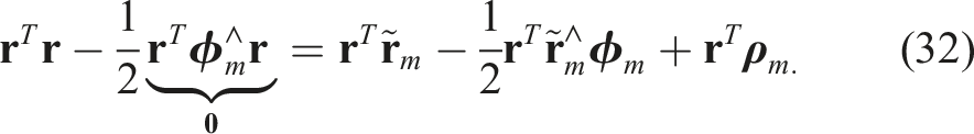
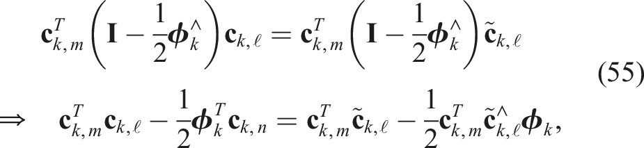
The key is that the second cubic term vanishes, leaving a new quadratic constraint that it is not simply a trivial linear combination of the existing constraints (Yang and Carlone, 2023). However, this constraint is redundant because it does not restrict the original feasible set at all. In the lifted SDP space it serves to restrict the feasible set and ultimately tighten the relaxation. Another useful redundant constraint can be formed by combining the last two of (31); the second last can be written as
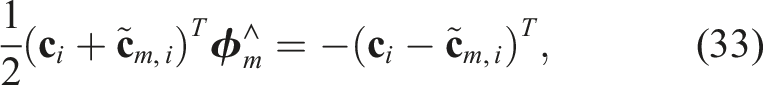
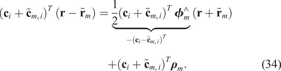
After performing the indicated substitution, this becomes
Summarizing, the following QCQP offers a reasonably tight SDP relaxation in practice:
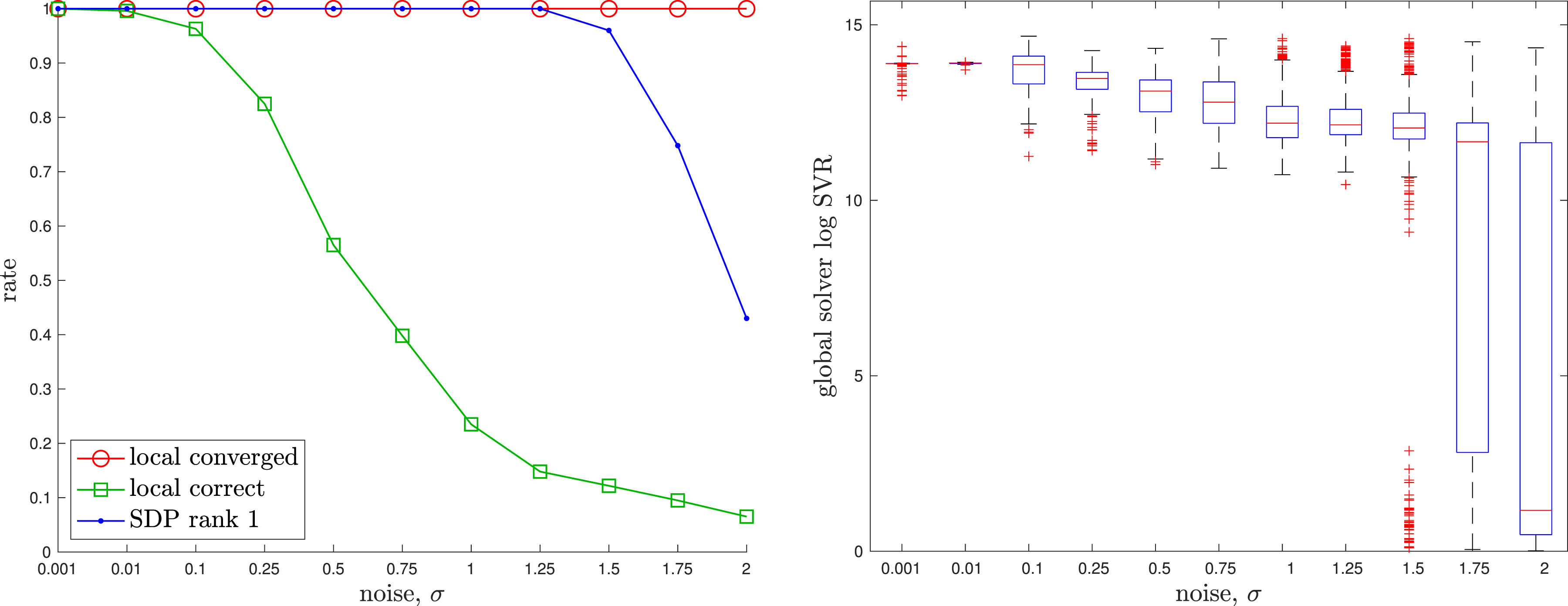
The appendix again provides a baseline local solver for this problem. For the global (SDP) solver we used Pose Averaging: Four examples of noisy pose averaging where the randomly initialized local solver (dotted) becomes trapped in a poor local minimum while the global solver (dashed) finds the correct solution, which is closer to the groundtruth pose (solid). The noisy pose measurements being averaged are shown in grey. Pose Averaging: A quantitative evaluation of the tightness of the pose averaging problem with increasing measurement noise level, σ. At each noise, we conducted 1000 trials of averaging 10 noisy poses. (left) We see that the local solver (randomly initialized) finds the global minimum with decreasing frequency (green) as the measurement noise is increased, while the SDP solver (blue) successfully produces rank-1 solutions (we consider log SVR of at least 5 to be rank 1) to much higher noise levels. For completeness, we also show how frequently the local solver converges to any minimum (red). (right) Boxplots of the log SVR of the SDP solution show that the global solution remains highly rank 1 over a wide range of measurement noise values.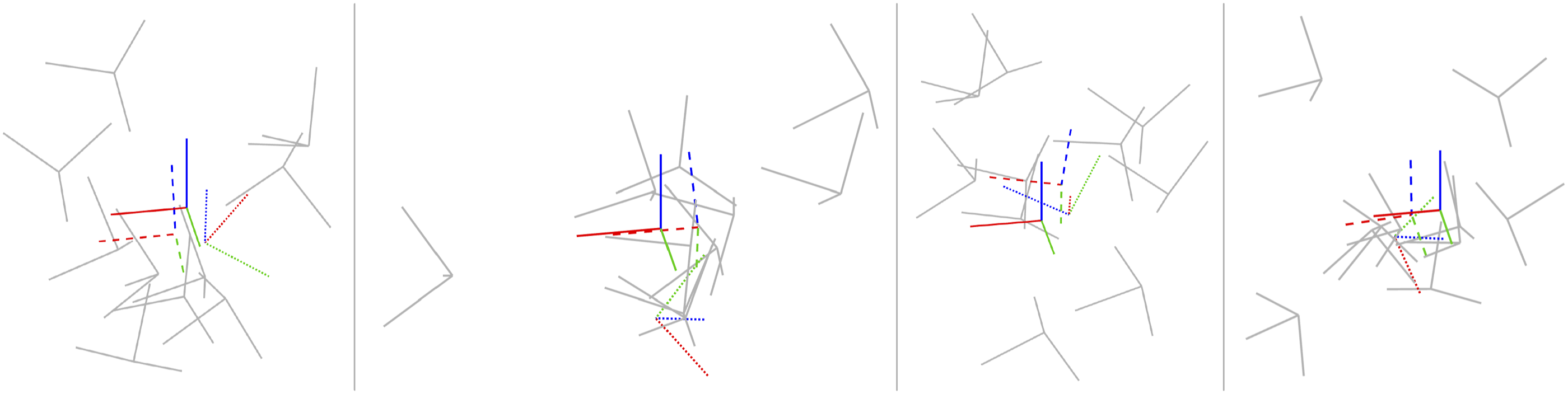
To justify the need for the redundant constraints, we conducted an ablation study (see Figure 6) wherein we varied the number of redundant constraints. The study shows that with more redundant constraints, we can tolerate a higher level of measurement noise while keeping the SDP tight. We always included the last redundant constraint in (36) as this enforces that the search space for the SDP remains compact
7
and it is therefore well posed. In the interest of space, we forgo similar ablation studies for the subsequent problems (discrete-time and continuous-time trajectory estimation), which reuse the pose averaging redundant constraints and then build on top of them. The studies are similar in that the more redundant constraints we add, the larger the noise region for which we can a priori predict that we will achieve rank-1 SDP solutions. Pose Averaging Ablation Study: Here we show the effect on SDP tightness of varying the number of redundant constraints in the pose averaging problem. The rightmost column shows our full set of recommended redundant constraints with the light-grey box indicating the region of measurement noise for which our problem can be deemed tight. The same grey box is shown in the other columns for reference, indicating that including fewer redundant constraints results in a lower level of noise for which we can keep the solution tight.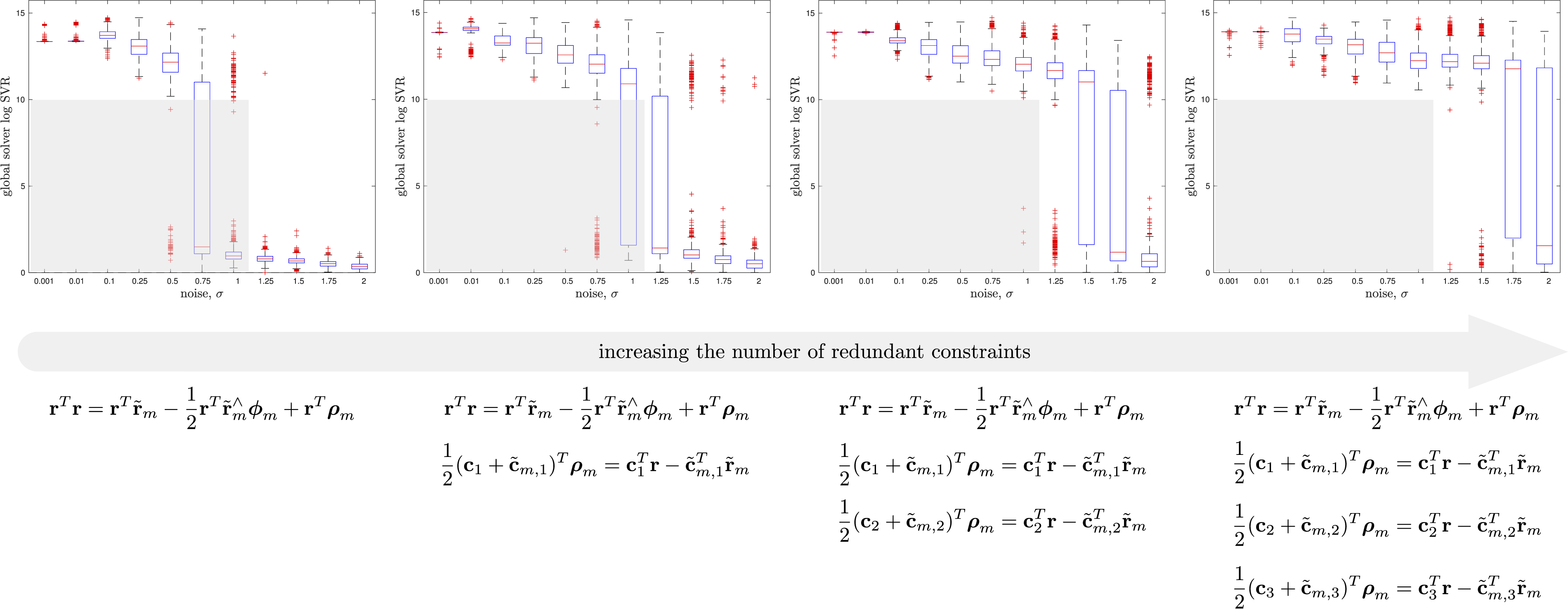
4. Discrete-time trajectory estimation
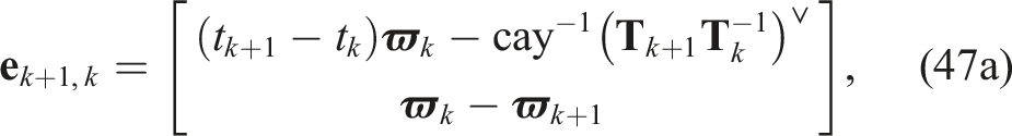
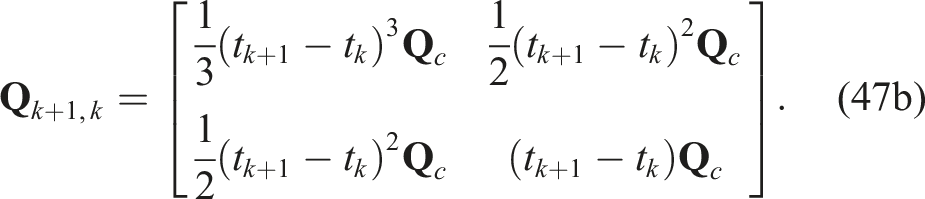
Our next problem is to consider estimation of a trajectory of K poses, Discrete-time Trajectory Estimation: Factor graph representation of the discrete-time estimation problem. Each black dot represents one of the error terms in the cost function of (37).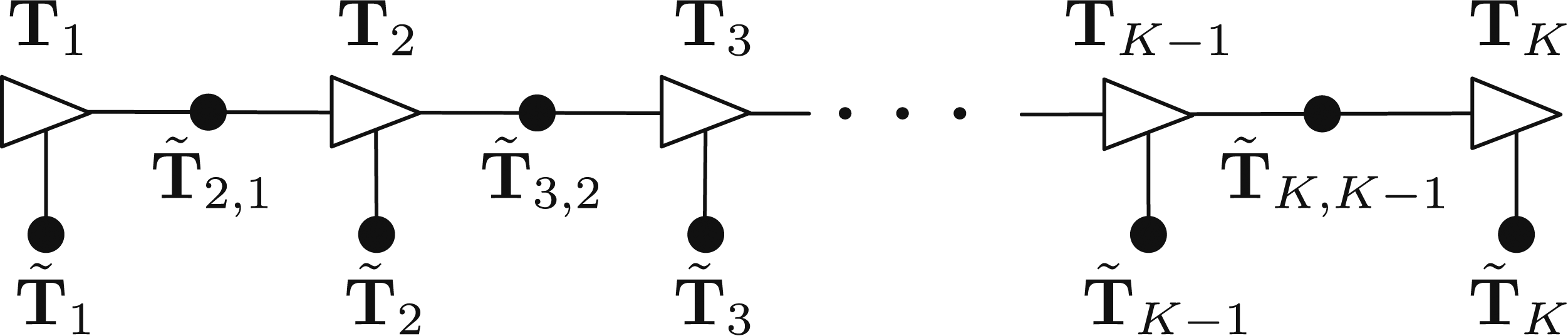
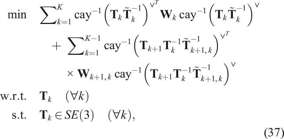
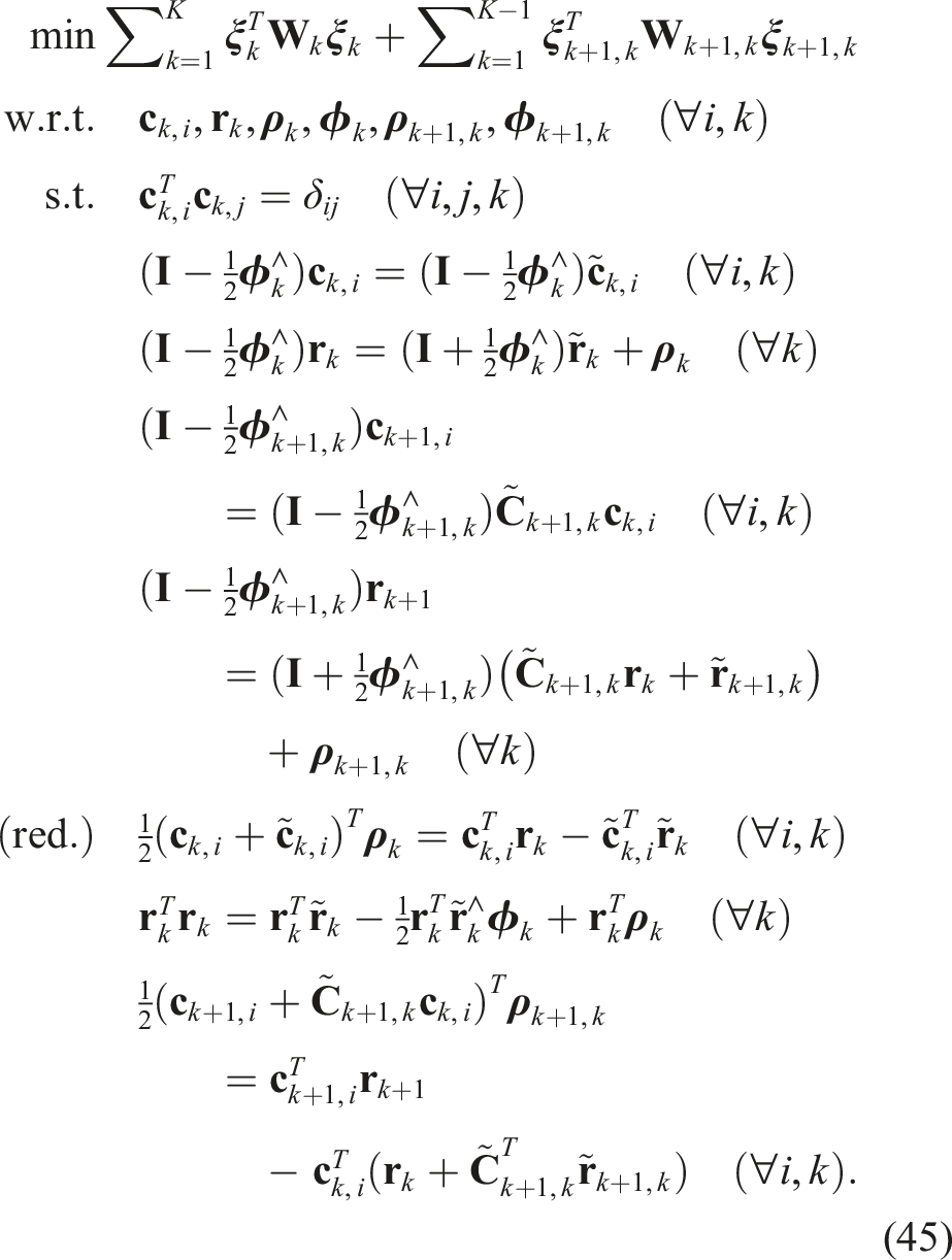
so that the optimization problem can be stated as a QCQP:
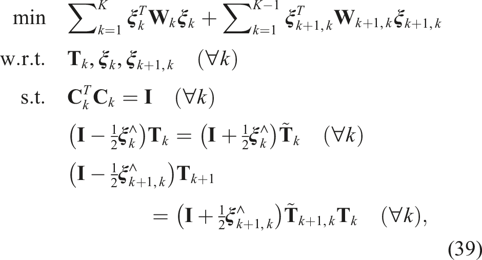
the QCQP optimization problem can be rewritten compactly as
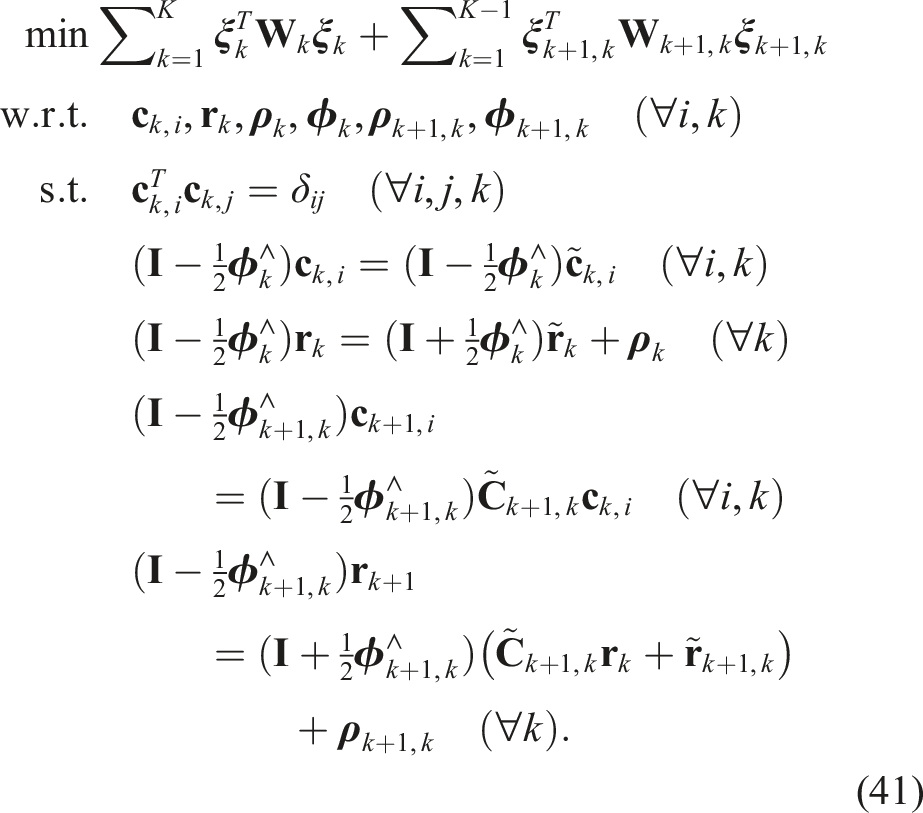
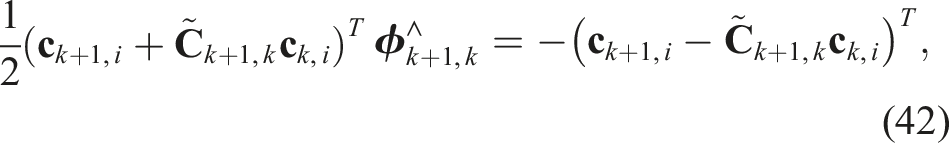
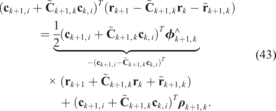
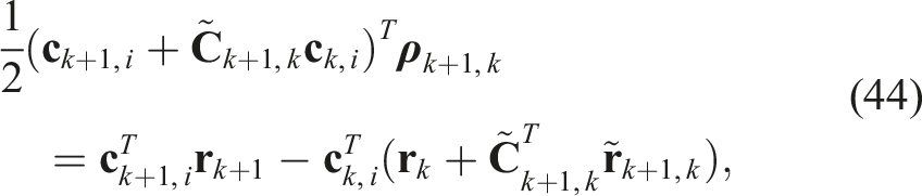
Similarly to the pose averaging problem, if we convert this QCQP to a SDP, it is not always tight even for low-noise levels. We need to include some redundant constraints to improve tightness. For each of the
Such additional redundant constraints can be formed by combining the last two of (41); the second last can be written as
Summarizing, the following QCQP offers a reasonably tight SDP relaxation in practice:
The appendix provides a baseline local solver for this problem. For the global (SDP) solver we used Discrete-time Trajectory Estimation: Two examples of discrete-time trajectory estimation where the randomly initialized local solver (red) becomes trapped in a poor local minimum while the global solver (green) finds the correct solution, which is closer to the groundtruth (blue). The noisy pose measurements are also shown (grey). It is interesting to note that the poor local solver solutions are twisted around the groundtruth. Discrete-time Trajectory Estimation: A quantitative evaluation of the tightness of the discrete-time trajectory estimation problem with increasing measurement noise, σ. At each noise level, we conducted 100 trials with the geometry of the trajectory as in the left example of Figure 8. (left) We see that the local solver (randomly initialized) finds the global minimum with decreasing frequency (green) as the measurement noise is increased, while the SDP solver (blue) successfully produces rank-1 solutions (we consider log SVR of at least 5 to be rank 1) to much higher noise levels. For completeness, we also show how frequently the local solver converges to any minimum (red). (right) Boxplots of the log SVR of the SDP solution show that the global solution remains highly rank 1 over a wide range of measurement noise values.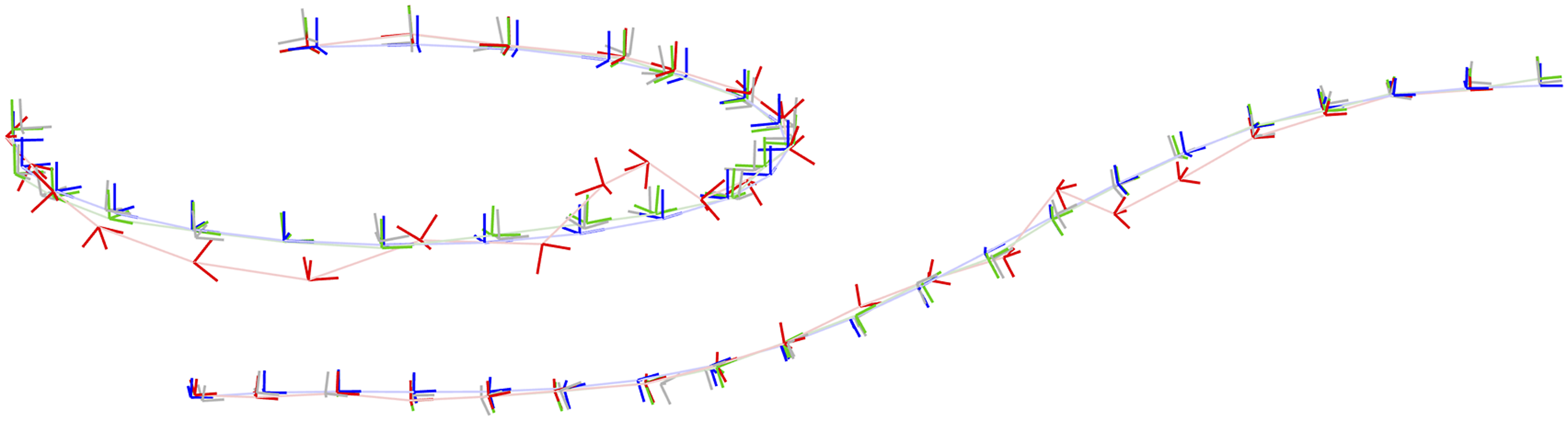
5. Continuous-time trajectory estimation
Finally, we consider so-called continuous-time trajectory estimation. Continuous-time methods come in parametric (Furgale et al., 2012) and nonparametric (Anderson and Barfoot, 2015; Barfoot et al., 2014) varieties; here we will discuss the latter. We consider a continuous-time Gaussian Process (GP) prior over the trajectory known as White Noise on Acceleration (WNOA); this serves to smooth the trajectory and is fused with pose measurements provided at discrete times. We will still ultimately have to discretize the trajectory for the purpose of estimation and so will have K states comprising both pose and generalized velocity (a.k.a., twist), Factor graph representation of the continuous-time estimation problem. Each block dot represents one of the error terms in the cost function of (46).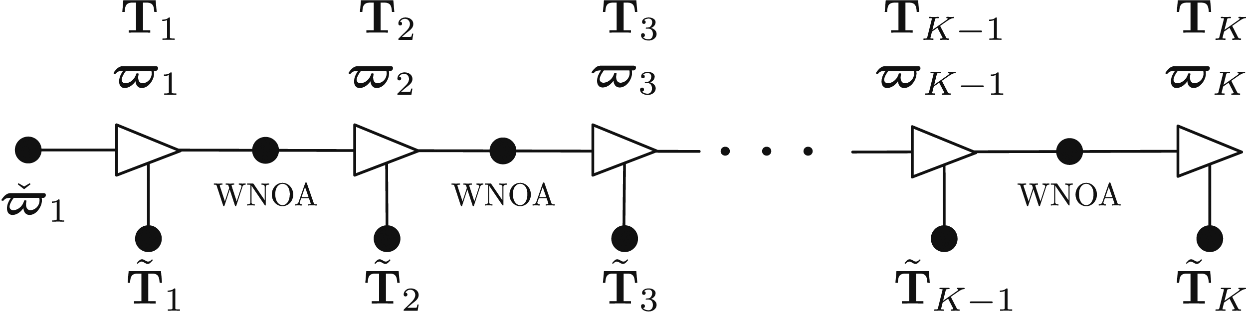
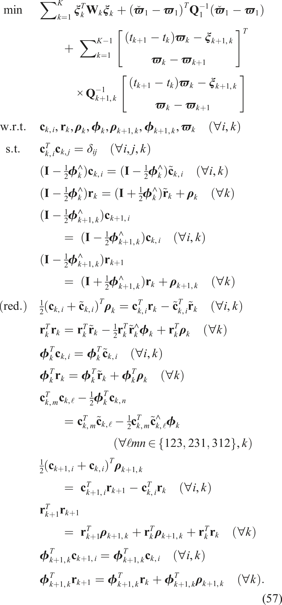
The optimization problem that we want to solve in this case is
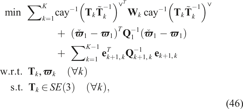
The t
k
are known timestamps of the states,
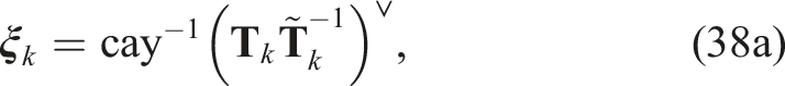
Similarly to the discrete-time trajectory estimation case, we introduce the following substitution variables
8
:
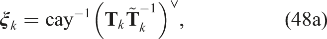

so that the optimization problem can be stated as a QCQP:
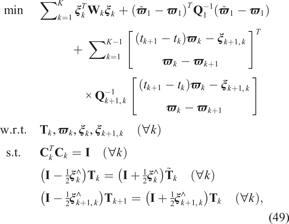


the QCQP optimization problem can be rewritten compactly as
Similarly to the problems above, if we convert this QCQP to a SDP, it is not tight even for low-noise levels. We need to include some redundant constraints to improve tightness. For each of the
We can generate some additional redundant constraints fairly easily. First, we can premultiply the second constraint of (51) by

Premultiplying the fourth and fifth constraints in (51) by


Next, we can exploit the fact that columns of a rotation matrix satisfy

Summarizing, the following QCQP offers a reasonably tight SDP relaxation in practice:
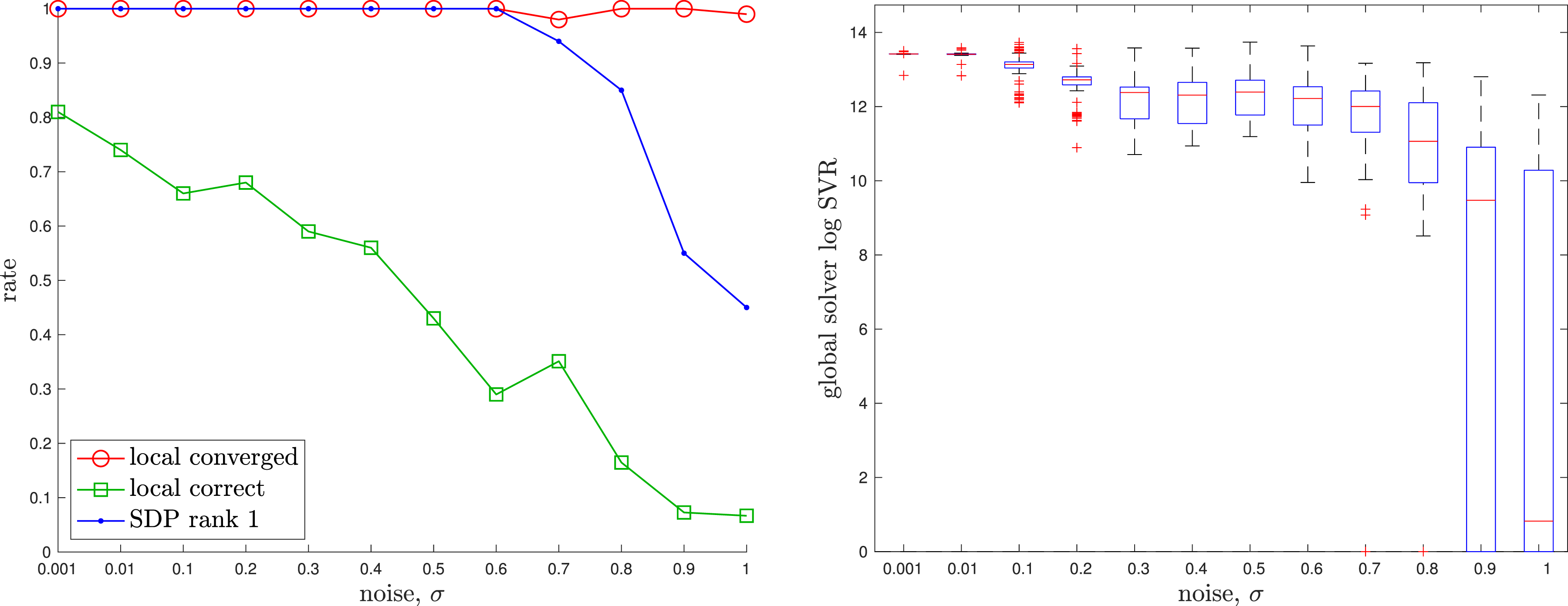
The appendix provides a baseline local solver for this problem. For the global (SDP) solver we used Continuous-time Trajectory Estimation: Four examples of continuous-time trajectory estimation where the randomly initialized local solver (red) becomes trapped in a poor local minimum while the global solver (green) finds the correct solution, which is closer to the groundtruth (blue). The noisy pose measurements (occurring only at the start, middle, and end of each trajectory) are also shown (grey). The local minimum in the leftmost example is very similar to one reported by Lilge et al. (2022). Continuous-time Trajectory Estimation: A quantitative evaluation of the tightness of the continuous-time trajectory estimation problem with increasing measurement noise, σ. At each noise level, we conducted 100 trials with the geometry of the trajectory as in the left example of Figure 11. (left) We see that the local solver (randomly initialized) finds the global minimum with decreasing frequency (green) as the measurement noise is increased, while the SDP solver (blue) successfully produces rank-1 solutions (we consider log SVR of at least 5 to be rank 1) to much higher noise levels. For completeness, we also show how frequently the local solver converges to any minimum (red). (right) Boxplots of the log SVR of the SDP solution show that the global solution remains reasonably rank 1 over a wide range of measurement noise values.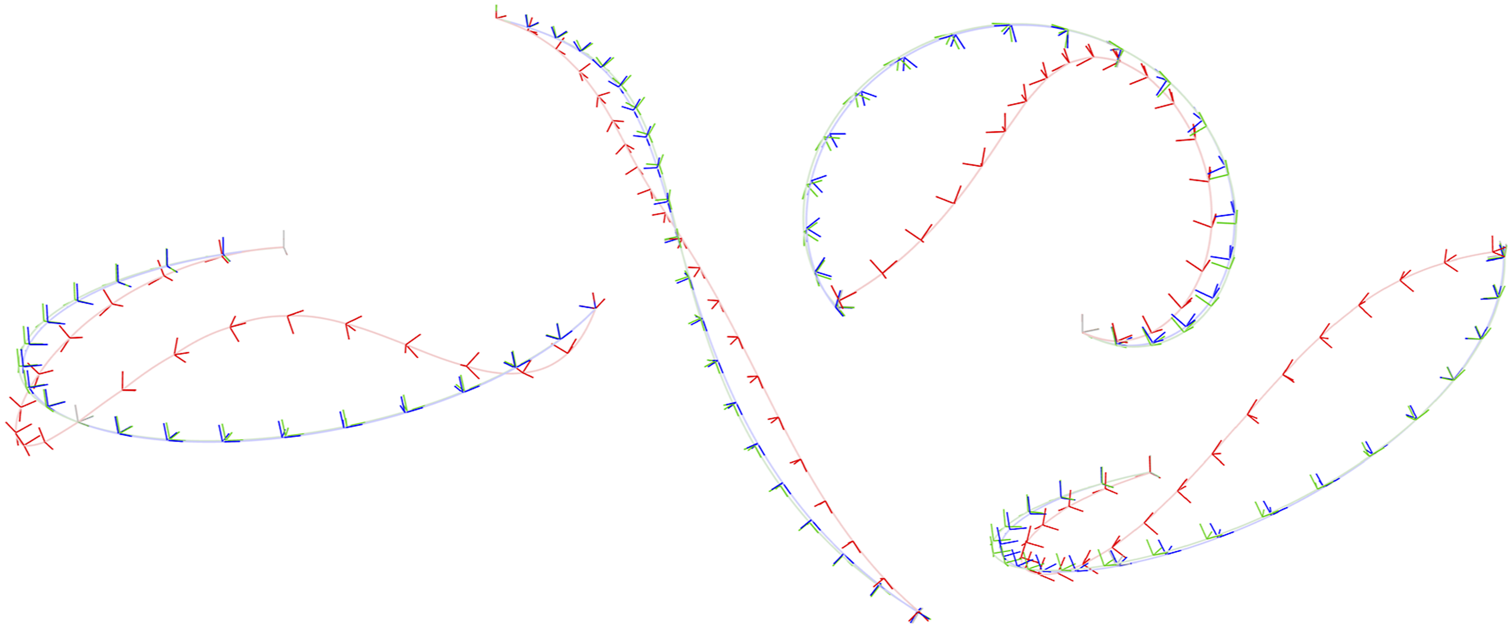
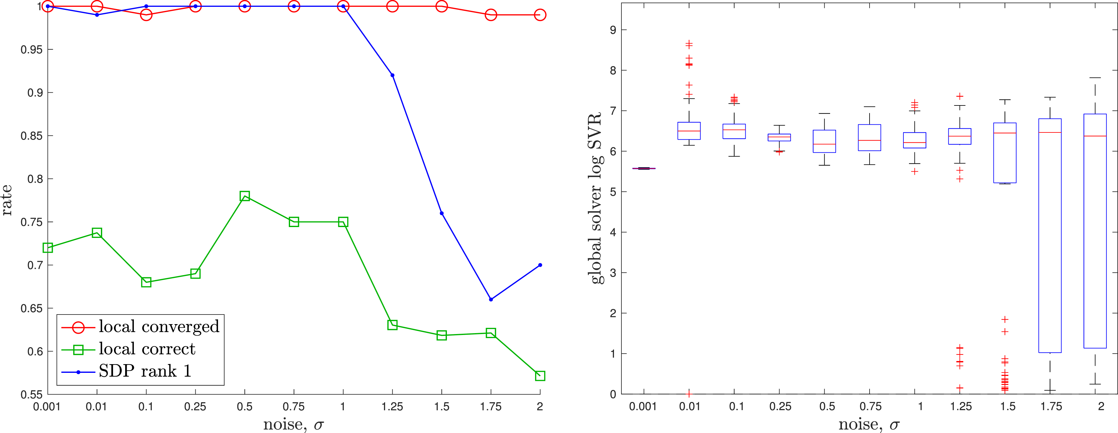
There are also a few noteworthy differences in the continuous-time experiment as compared to the discrete-time case. First, the log SVR values are quite a bit lower in Figure 12 as compared to Figure 9. This seems to be mainly due to the fact that we are now using a sparser set of measurements. Our continuous-time experiments had pose measurements only at the start, middle, and end, whereas the discrete-time case had pose measurements at every timestep. It is known that a sparser measurement graph can impact SDP tightness (Holmes and Barfoot, 2023). Second, the low-noise test cases experienced some numerical issues with getting the SDP solver to reliably converge. It seems this is related to matrix conditioning resulting from the fact that we are marginalizing out the
6. Conclusion and future work
We have presented several new convex relaxations for pose and rotation estimation problems based on the Cayley map. Our results indicate that for small problem sizes, we can successfully achieve global optimality with realistic amounts of noise and even with measurement sparsity in the case of continuous-time trajectory estimation. In each of the experiments, we indicated that covariance of the error associated with each pose measurement cost term is σ2
While our results are promising, we are still relying on off-the-shelf solvers once our problem has been converted to an SDP, which means that we will not be able to scale up to extremely large state sizes. To scale up, there are a few possibilities that we could explore. First, perhaps we might be satisfied with merely certifying our local solver solutions. Other works have focussed on this. The challenge is that in most of the problems of this paper, we require redundant constraints to tighten our SDPs. This means that we do not meet the technical condition of Linearly Independent Constraint Qualification (LICQ) (Boyd and Vandenberghe, 2004). It turns out that this makes it more challenging to calculate an optimality certificate. Yang et al. (2021) is a practical example where a certificate has been constructed for this type of situation, but there are still scaling issues. Another possibility is to solve our problems globally using the approach of Burer and Monteiro (2005) (studied more recently by Boumal et al. (2016)). This was exploited with very impressive results by Rosen et al. (2019); Dellaert et al. (2020); however, these problems enjoyed LICQ. To our knowledge, this approach has not been applied to problems in robotics with redundant constraints. Or, perhaps generic SDP solvers can be made to better exploit problem-specific structure (e.g., chordal sparsity). We plan to explore these and other ways of scaling global optimality for a larger range of state estimation problems.
Footnotes
Declaration of conflicting interests
The author(s) declared no potential conflicts of interest with respect to the research, authorship, and/or publication of this article.
Funding
The author(s) disclosed receipt of the following financial support for the research, authorship, and/or publication of this article: This work was supported by the Swiss National Science Foundation, Postdoc Mobility under Grant 206954 and in part by the Natural Sciences and Engineering Research Council of Canada (NSERC).