
Abstract
Independent robotic manipulation of two large permanent magnets, in the form of the dual External Permanent Magnet (dEPM) system has demonstrated the possibility for enhanced magnetic control by allowing for actuation up to eight magnetic degrees of freedom (DOFs) at clinically relevant scales. This precise off-board control has facilitated the use of magnetic agents as medical devices, including catheter-like soft continuum robots (SCRs). The use of multiple robotically actuated permanent magnets poses the risk of collision between the robotic arms, the environment, and the patient. Furthermore, unconstrained transitions between actuation inputs can lead to undesired spikes in magnetic fields potentially resulting in unsafe manipulator deformation. This paper presents a hybrid approach to trajectory planning for the dEPM platform. This is performed by splitting the planning problem in two: first finding a collision-free physical path for the two robotically actuated permanent magnets before combining this with a path in magnetic space, which permits for a smooth change in magnetic fields and gradients. This algorithm was characterized by actuating each of the eight magnetic DOFs sequentially, eliminating any potential collisions and reducing the maximum undesired actuation value by 203.7 mT for fields and by 418.7 mT/m for gradients. The effect of this planned magnetic field actuation on a SCR was then examined through two case studies. First, a tip-driven SCR was moved to set points within a confined area. Actuation using the proposed planner reduced movement outside the restricted area by an average of 41.3%. Lastly, the use of the proposed magnetic planner was shown to be essential in navigating a multi-segment magnetic SCR to the site of an aneurysm within a silicone brain phantom.
1. Introduction
Magnetic control of robots offers a range of advantages; notably, forces and torques are applied remotely allowing for almost limitless miniaturization. This possibility to reduce robot scale makes magnetic actuation well suited to medical applications. Magnetic actuation has been demonstrated for control of capsules (Kim et al., 2024), surgical tools (Kladko and Vinogradov, 2024), and microrobots (Bozuyuk et al., 2023) amongst others. This offers the potential for navigation (Kim et al., 2019; Jeon et al., 2019) and therefore drug delivery (Wu et al., 2022) or other treatments in previously inaccessible areas (Jeon et al., 2019).
These benefits can be further exploited through magnetically actuated soft continuum robots (SCRs). SCRs have the potential to be transformative in the healthcare field. The physically soft structure of such devices allows for conformity to natural, curvilinear pathways within organs, vessels, and potentially even in extracellular spaces. Minimising disruption of the native anatomy when performing medical procedures has been shown to reduce trauma, pain, and recovery times (Dupont et al., 2021). SCRs have been proven to be effective in applications such as bronchoscopy (Edelmann et al., 2018), cardiovascular interventions (Yang et al., 2021; Jeon et al., 2019; Ali et al., 2016), and insertion of cochlear implants (Bruns et al., 2020).
For applications requiring highly precise and delicate navigation of convoluted anatomical pathways such as neurosurgery (Figure 1), there is a benefit in moving beyond point control (tip-driven SCRs) towards increased controllable degrees of freedom (DOFs). This characteristic has been demonstrated for pneumatic SCRs among others (Whitesides, 2018) but remains elusive in the realm of magnetic actuation. Minimally invasive magnetic robot-assisted surgery allows for access to aneurysms by utilising the brain’s native endovascular structure whilst avoiding injury to the brain parenchyma. This illustration demonstrates how a modified SCR can be navigated to the desired location, through which endovascular coiling can be performed (where microcatheter-delivered coils are deployed into the aneurysm, with the aim of blocking blood flow to the aneurysm). This illustration was created using BioRender.com.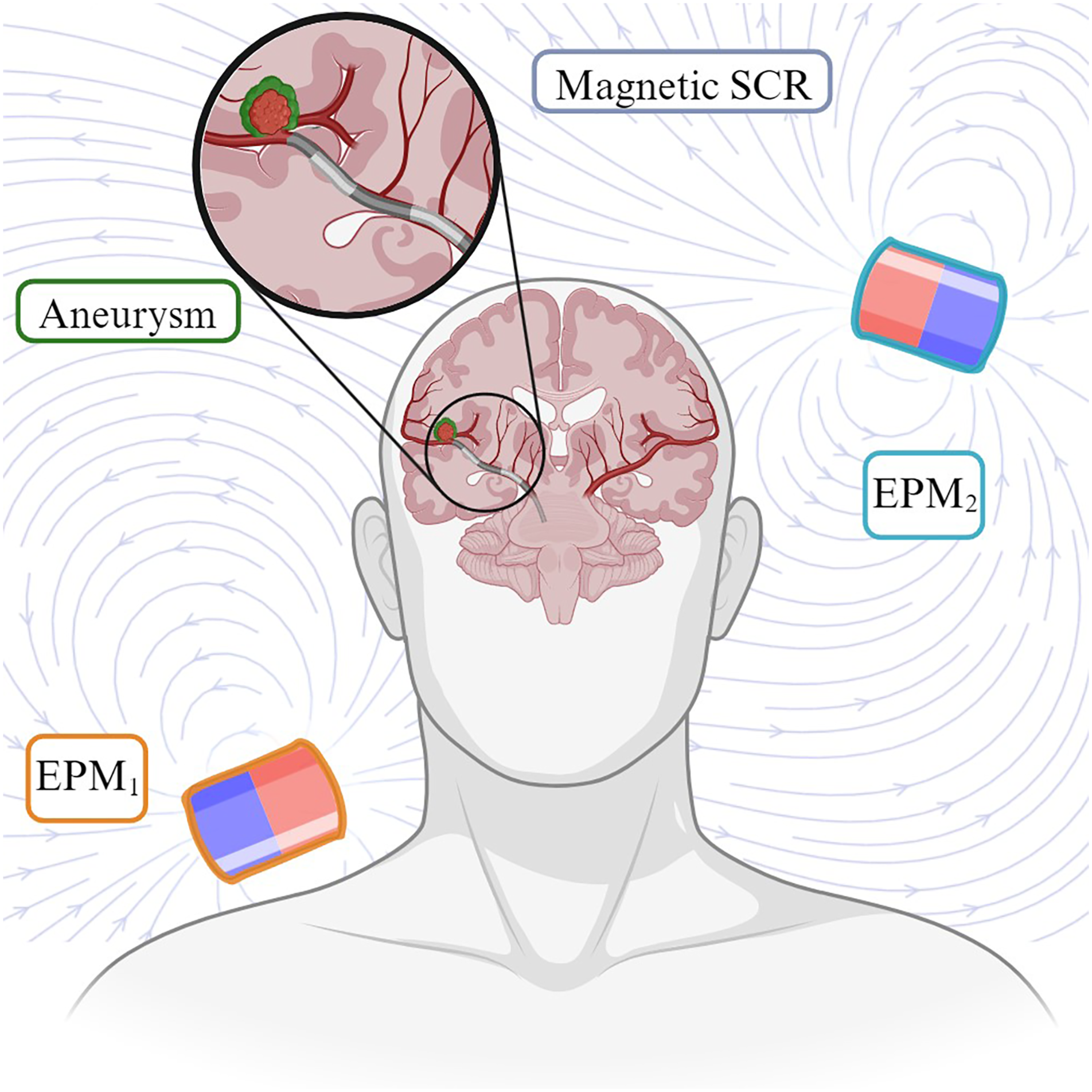
Salmanipour and Diller (2018) show how forces and torques can be independently induced on magnetic agents by controlling the magnetic field and gradient. This multi-DOF actuation can be exploited to achieve full shape and pathway control (important for endovascular navigation). Multi-DOF control of magnetic agents has been shown using systems of coils (Boehler et al., 2023; Bruns et al., 2020; Hoang et al., 2021; Hong et al., 2020; Richter et al., 2021; Salmanipour et al., 2021); however, these systems are typically associated with large, static equipment, small workspaces, up-scaling limitations, and high running costs (da Veiga et al., 2020). The use of External Permanent Magnets (EPMs) allows for the generation of magnetic fields and gradients free from these constraints, thus allowing for a larger workspace (Pittiglio et al., 2022) although a single EPM only allows for a maximum of five DOF control (Kim et al., 2019). Multiple points along a magnetic SCR can be controlled by a single EPM when having each segment oppositely magnetized (Lin et al., 2023); however, the overall independently controllable DOFs are still limited to five.
Multi-EPM actuated systems (Carpi and Pappone, 2009; Ryan and Diller, 2017) have demonstrated five and six DOF control, respectively. However, the dual External Permanent Magnet (dEPM) platform, which uses two robotically actuated EPMs as described in Pittiglio et al. (2023), is the only example of an EPM system that has been shown to actuate the minimum eight magnetic DOFs required to independently control the force and torque on a magnetic object within a confined workspace.
Unlike coil-based systems, the use of robotic manipulators to control the pose of EPMs introduces a non-linear relationship between the robot configuration and the resulting magnetic field. This approach often leads to the production of undesired fields and gradients when transitioning between robot poses. This can lead to an inadvertent change in pose of the SCR, potentially altering its navigation, triggering an unintentional release in payload and/or harming the patient (potentially life-threatening in clinical applications such as neurosurgery). Furthermore, the introduction of robotically actuated EPMs into a sensitive environment such as an operating theatre may bring about additional risks if the movement of these devices is not correctly managed.
Trajectory planning involves finding an ideal route from a start point to an end point while avoiding obstacles. Trajectory planning has been widely used in the field of robotics, from planning for single multi-DOF robotic manipulators (Ataka et al., 2022; Porges et al., 2021), for multiple robots (Yan et al., 2013), as well as for other medical continuum robots (Hoelscher et al., 2021). Furthermore, neuronavigation is routinely used in neurosurgical clinical practice. Thus, translating trajectory planning using existing brain volumetric imaging, hardware and software is eminently feasible. However, planning to reduce undesired magnetic actuation while avoiding obstacles for the dEPM or similar EPM platforms has yet to be addressed.
This paper introduces a hybrid approach for trajectory planning for the dEPM and similar multi-EPM based platforms. The proposed algorithm takes into account the temporal change in magnetic field space as well as generating a collision-free path in the operational space. The efficacy of this trajectory planner was demonstrated on the dEPM platform where two EPMs are each mounted on a seven-DOF robotic manipulator. Here the objective is to minimize the deviation from the desired magnetic field while preventing collision between the manipulators. This was demonstrated by first analyzing the change in magnetic field and gradient with and without the use of the proposed trajectory planner. The effect of controlled and collision-free magnetic actuation delivered by the trajectory planner was subsequently visualized through two case studies. First, through the control of a SCR with single uniform magnetic segment at its tip. The second case study demonstrates the combined safe operation and predicable magnetic field and gradient generation in a clinical context by applying the planner to the navigation of a multi-magnet SCR to the site of an aneurysm within a soft brain phantom.
2. Magnetic actuation
An external magnetic field
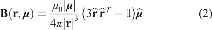
Taking the partial spatial derivative of (2), the magnetic gradients can be calculated as
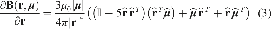
Assuming that the workspace is free from any other magnetic objects and free of currents, Maxwell’s equations will apply as
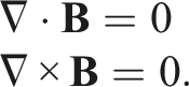
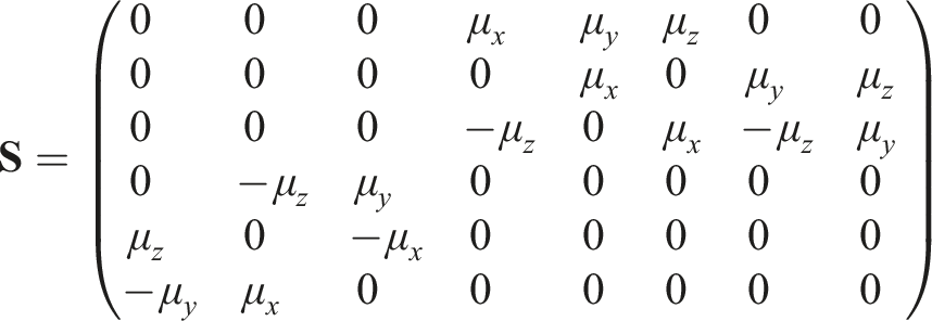
According to these conditions, matrix (3) must be symmetric and have zero trace and therefore can be expanded as
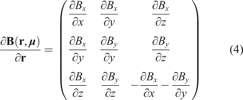
As shown by Petruska and Nelson (2015), the gradient matrix (4) thus has five independent components, these being
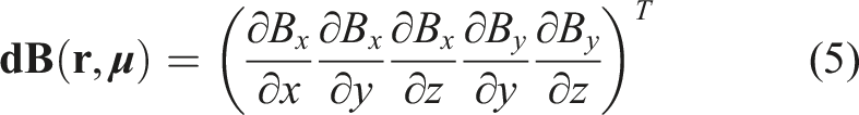
Stacking the field elements with these gradient elements, the eight independently controllable magnetic DOFs can be grouped into the magnetic field vector
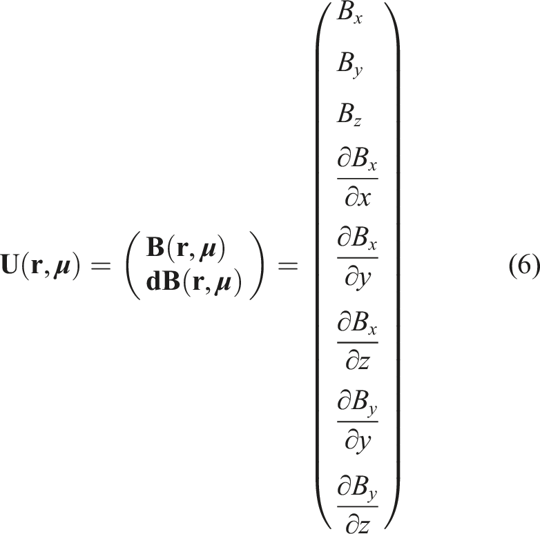
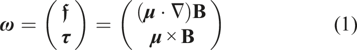
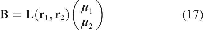
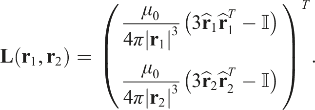
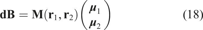
By substituting (6) into (1) and expressing the

where
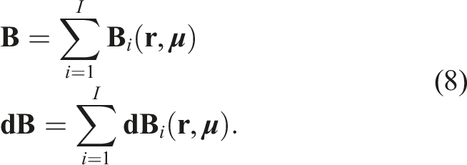
This can be generalized for any number (I) of EPMs by using the superposition principle, such that
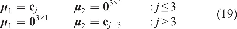
Independent control of each component of
3. Motion planning
Before delving into the trajectory planning algorithm proposed, we first define the terms used. Operational space refers to a coordinate system which defines the position and orientation of an object. Magnetic space is defined as the change of magnetic field and gradient with respect to time and position. A path is a set of points in either operational or magnetic space that we intend to follow. A trajectory is defined as a path on which a timing law is specified, typically by means of velocities or accelerations at each point. A trajectory planner algorithm takes a path description along with any constraints (in any domain) and outputs an end-effector trajectory as a time sequence. Using these definitions, we can move on to defining the trajectory planning problem for the dEPM platform.
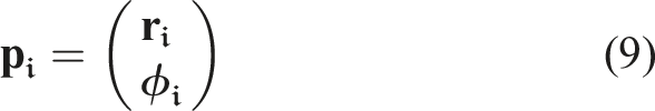
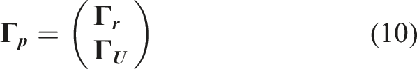
To avoid undesired cross-activation of magnetic DOFs with EPMs, careful planning of their motions is required. The planner will define a series of poses for each EPM such that the path is collision-free and the magnetic field vector generated throughout the EPMs’ trajectory tracks a chosen path in magnetic space. We define the pose of the ith EPM in the operational space as
The challenge of generating trajectories could be solved by formulating as a differential control problem. Here, the input variables would be defined in joint space (the joint angles of the robots actuating the EPMs) and the Jacobian would be calculated with respect to the applied magnetic field vector in the workspace. However, for this platform, this can lead to solutions which suffer from local minima as well as provoking magnetic instability. The consequence of this being that small variations in the EPMs’ position results in large differences in magnetic field.
Another possible approach would be to alter a popular trajectory planning algorithm such as rapidly exploring random trees (Ge et al., 2016; Wei and Ren, 2018), probabilistic road-map planning (Bohlin and Kavraki, 2000; Sánchez and Latombe, 2002; Geraerts and Overmars, 2004) and grid based search methods (Ataka et al., 2022; Sturtevant, 2012) to take into account both a magnetic and positional cost object. However, the exhaustive nature and high time complexity of these algorithms, along with the large number of control variables associated with our system (14 robot joints, 8 magnetic DOFs) combined to make such algorithms inefficient.
Obstacles are easier to describe in operational space than in the corresponding joint space. Additionally, when fidelity to a chosen path in operational space is prioritized, planning directly in task space is suggested (Siciliano et al., 2010). Trajectory planning in operational space ensures the end-effector position is not subject to the non-linear effects introduced by direct kinematics. Thus, we designed our planning algorithm in operational space and applied standard inverse kinematic solvers for generation of joint space trajectories.
3.1. Planning in operational space
The trajectory planner aims to find a operational space path of EPM poses ( The trajectory planning process visualized through a flowchart. Processes taking part in operational space are grouped in the blue box, while those taking place in magnetic space are grouped in the purple box. The start and end EPM poses (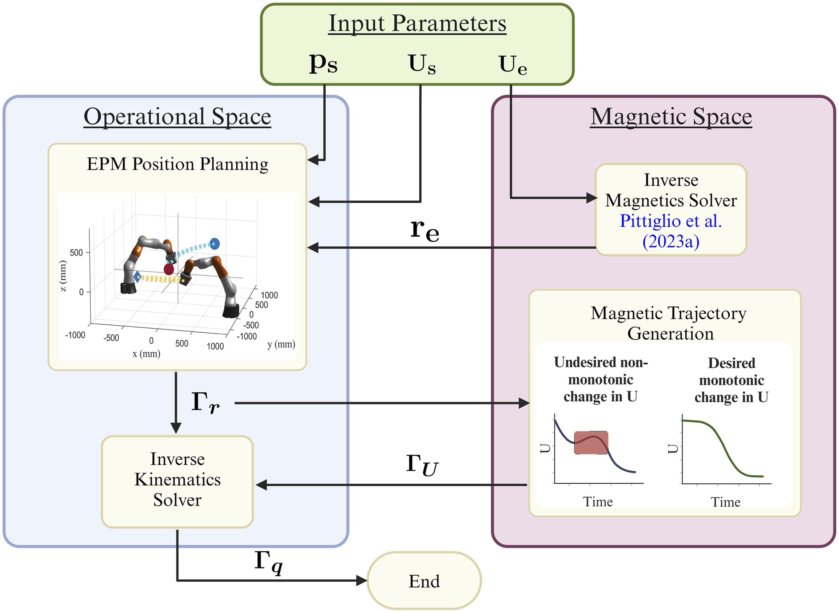
The planning process, along with the transition between spaces can be visualized by the flowchart shown in Figure 2.
3.1.1. EPM position planning
For safe operation of the dEPM platform, two sets of obstacles need to be considered. The first obstacle is a sphere with a radius of 15 cm around the centre of the workspace. This represents the volume in which the magnetically actuated agent will be placed and thus must remain free of both EPMs and robotic manipulators. The second set of obstacles relates to the EPMs themselves. Due to the fact that permanent magnets cannot be ‘switched off’, it is crucial that each EPM is kept out of the path of, and at a safe distance from, the other EPM. If the EPMs are allowed in close proximity, the magnetic forces and torques may overcome the payload of the robotic manipulators, potentially damaging the robots themselves as well as anyone or anything else present in the workspace. A graphical representation of the dEPM platform and the obstacles considered can be seen in Figure 3. Graphical representation of the dEPM platform, generated paths with k = 3 and obstacle in the middle of the workspace. (a) View of platform from above with visualization. (b) View of platform from the Z–Y axis.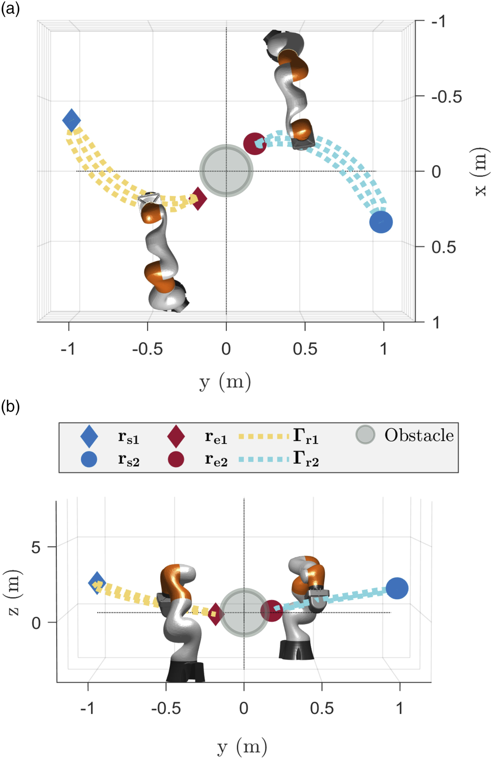
Considering the symmetry of the dEPM platform and the position of obstacles, we generated an operational space trajectory for the EPMs using spherical coordinates. This allows for easy representation of the obstacle in the middle of the workspace. By applying a spherical constraint to each EPM on opposite sides of the workspace, EPM-to-EPM collision could be easily avoided. The planning task begins by calculating the start position (

To create spherical paths between
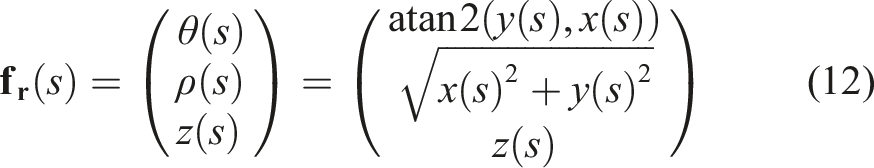
Here, θ, ρ, and z represent the axis of the spherical domain while x, y, and z are the axes of the Cartesian coordinate system, with both these coordinate systems forming part of the operational space. By linearly interpolating between the start and end point in spherical space we ensure that each EPM travels in a circular trajectory around the centre of the workspace, without colliding with the other EPM.
3.1.2. Planning in magnetic space
To allow for a smooth transition in magnetic space, k obstacle-free operational space paths for each EPM are generated with varying values of ρ(s). For every value of s, k different positions are generated. The generation of k different paths gives the opportunity to the motion planning algorithm to choose a waypoint sitting on any one of the generated paths. This allows for a change in EPM position, within a collision-free space, which satisfies the desired change in magnetic actuation. Figure 3 shows the dEPM platform following a trajectory planned to transition between an arbitrary start and end pose with k = 3.
Once k paths containing the potential positions of the EPMs have been generated, optimization of the orientation of the EPMs can begin. The first step involves creating a desired path in magnetic space (

where
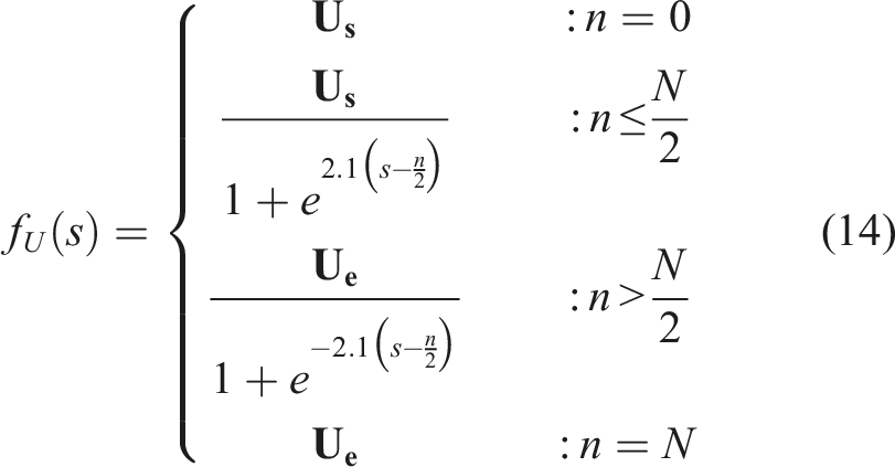
The numerical values shown in (14) were empirically tuned. These values represent how quickly the magnetic field changes across the magnetic path. This is dependent on the speed at which the EPMs are physically able to move, and therefore is a platform specific parameter. This produces a magnetic path where the magnitude of the generated magnetic actuation (|
Having generated the required EPMs positions through


Similarly, by applying (4) and (8) to the magnetic gradients generated by two EPMs
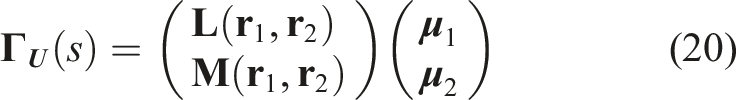
By knowing the position of each EPM at every waypoint as well as
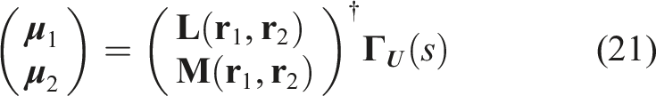
Using (21),

3.2. Joint trajectory generation
By combining operational space and magnetic space planning, optimal trajectories for the EPMs avoiding collisions and producing desired magnetic actuation can be generated. Having found the optimal position and orientation for both EPMs, the next step involves finding the corresponding joint positions for two robots in order to follow the chosen path. Desired joint angles are found via standard inverse kinematic solvers and are constrained to find solutions that avoid collisions between the robot and the central workspace (Robotics Toolbox, MATLAB, MathWorks). Due to the use of a 7 DOF arm to control the 5 DOFs of each EPMs, there is inherent redundancy in kinematic solutions, therefore solutions are constrained to be close in joint space to the previous pose. Once joint space solutions are obtained for the desired poses, they are interpolated using Piece-wise Cubic Hermitean Interpolation Polynomials (PCHIP) (Kahaner et al., 1989) to produce smooth trajectories (
3.3. dEPM Platform
The dEPM platform uses two seven-DOF robots manipulating two axially magnetized, cylindrical N52 EPMs (101.6 mm diameter and length) and can be seen in Figure 4(a). This platform is capable of safely generating fields of up to 200 mT and magnetic gradients of up to 500 mT/m. Pittiglio et al. (2023) show how the dEPM platform is capable of accurately generating different combinations of magnetic fields and gradients with 81.1% random field and gradient combinations. Due to the safety risk presented by the unplanned manipulation of the EPMs, the robotic manipulators were restricted to only operate at 30% of their maximum operating speed. The dEPM platform is equipped with a four-camera optical tracking system (OptiTrack, NaturalPoint, Inc., USA) as seen in Figure 4(a). The tracking setup serves a dual purpose; first, it plays a critical role in calibrating the dEPM platform by determining the centre of actuation. This calibration process involves capturing the position of optical markers strategically placed near the desired centre of actuation. Second, the tracking setup enables real-time monitoring of moving objects (such as SCRs) facilitating the analysis of their positional changes in response to magnetic influence. To make this setup more accommodating for the medical field, these procedures could be replaced by alternative sensing methods such as Fiber Bragg Gratings (FBGs) and magnetic localization. Setup for measuring magnetic fields and gradients. (a) dEPM platform including optical calibration system, with sensor board placed in the middle of the workspace. (b) Sensor board with three 3D Hall effect sensors, used to measure magnetic fields and gradients.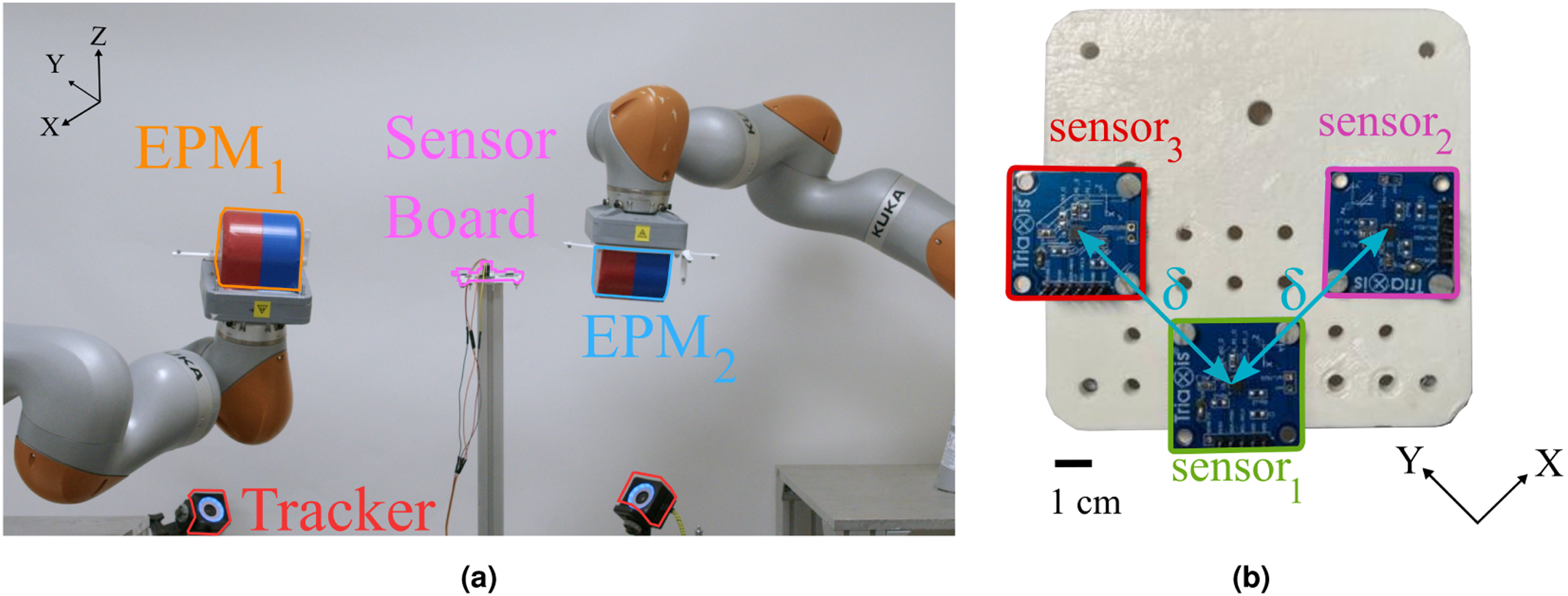
4. Eight DOF actuation
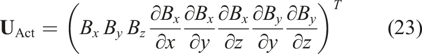
Independent magnetic field and gradient control is a key factor when controlling magnetic agents. This is due to the possibility to induce independent magnetic forces and torques. Therefore, to determine the performance of the proposed planner, the dEPM platform was subjected to the control task of sequentially actuating every component of (6) independently. Eight different values of
4.1. Methods and experimental setup
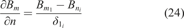
The magnetic fields and gradients were measured using the magnetic sensor arrangement shown in Figure 4(b). This consists of three 3D Hall effect sensors (MLX90395, Melexis, Belgium. Sensing range ±50 mT; Sensitivity 2.5 μT/LSB16, Footprint 3 × 3 × 0.9 mm). The position of sensor1 is considered to be in the centre of the workspace. The other sensors were placed a distance
4.2. Results
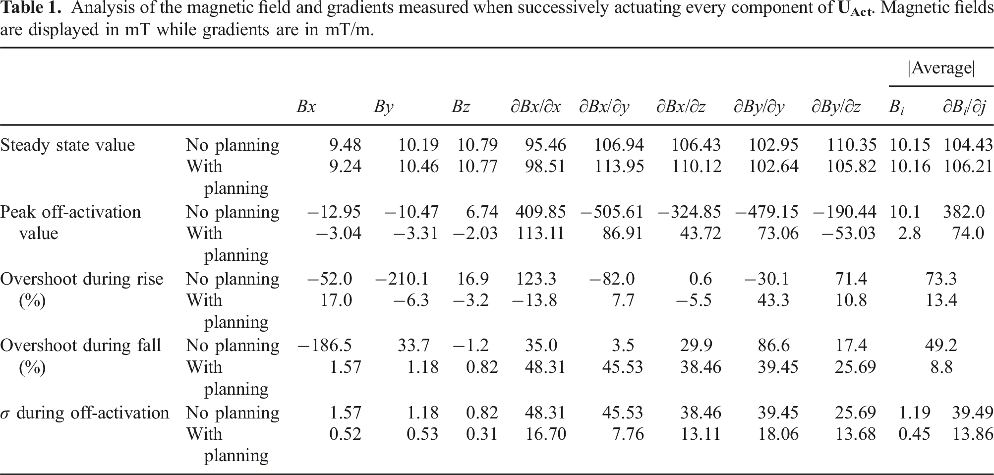
A comparison of the measured magnetic fields and gradients, with and without planning, are presented in Figure 5. For experiments performed without planning, an end pose was specified for each EPM and the default trajectory controller within each robotic manipulator was allowed to formulate the required trajectory. Throughout this paper, this approach is referred to interchangeably by the term magnetic agnostic planning. A quantitative analysis of these results can be found in Table 1. The difference in EPMs movement between the two experiments can be seen in Supplemental Video 1. The results between the no planning and the planning experiments were compared by taking an average of the absolute value of the magnetic fields and gradients (where applicable). Magnetic fields and gradients using the default magnetic agnostic planning and with the presented hybrid planner. The first row shows the actuation sequence Analysis of the magnetic field and gradients measured when successively actuating every component of 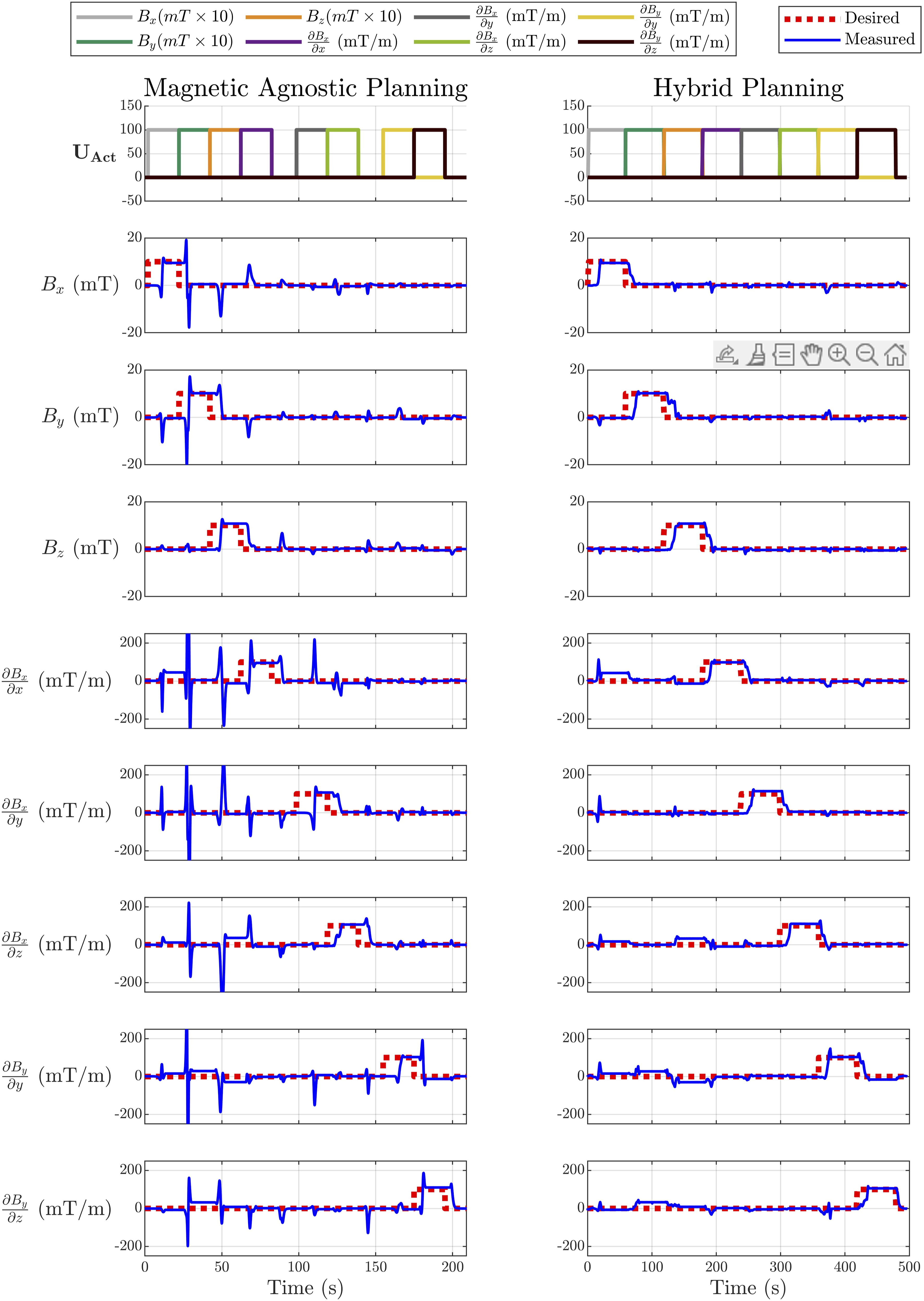
Through the use of the trajectory planner, every component of
By further analysing the field and gradients recorded, we can see that the steady state value, that is, the magnetic field or gradient value measured once the EPMs reached their final pose, matched the value set out at the beginning of this experiment for both the no planning and planning scenarios. The error associated with the steady state value (magnetic agnostic planning; 1.5% for fields, 4.4% for gradients, planning; 1.6% for fields, 6.21% for gradients) can be attributed to the errors related to the optical calibration method used.
The peak off-activation value refers to the maximum magnetic field and gradient measured when no actuation was requested. Table 1 shows that by using the proposed path planner the average peak off-activation can be reduced from 10.1 mT to 2.8 mT for fields and from 382.0 mT/m to 74.0 mT/m for gradients.
The maximum amount by which the magnetic field and gradient overshot or undershot the desired value during the rise and fall times was also analysed. The rise time is defined as the time from when the change of magnetic field was requested, until steady state activation was recorded. The fall time is defined as the time between when the desired actuation of (23) is set to 0, until a constant value close to 0 (± 0.5 mT or ± 5 mT/m for gradients) was measured. Overshoots are defined as the amount the field or gradient surpassed the desired value, as a percentage of the desired value, while undershoots are the amount by which the magnetic field or gradient was actuated to a negative value, as a percentage of the desired value. In Table 1, undershoots are represented by a ‘−’ sign. The use of the proposed path planner was shown to drop the average overshoot/undershoot value from 73.3% to 13.4% during the rise time, and from 49.2% to 8.8% during the fall time.
The standard deviation (σ) during the off-activation period was also compared. This represents how much the magnetic field and gradient differ from the zero value when no activation is requested. Therefore, a σ of 0 is desired for the optimal case. The magnetic planner reduced the σ from 1.19 mT to 0.45 mT for fields and from 39.49 mT/m to 13.86 mT/m for gradients.
Information on how the activation of a single DOF affects the other DOFs is shown in Figure 6. This figure shows the maximum field or gradient measured during the rise time of each actuation, referred to as cross-activation. This time period was analyzed as it portrays the time when the EPMs are in transition from one pose to another. The measured values are represented as percentages of the desired field or gradient. Two DOFs are shown to be active for each component of Cross-activation of each 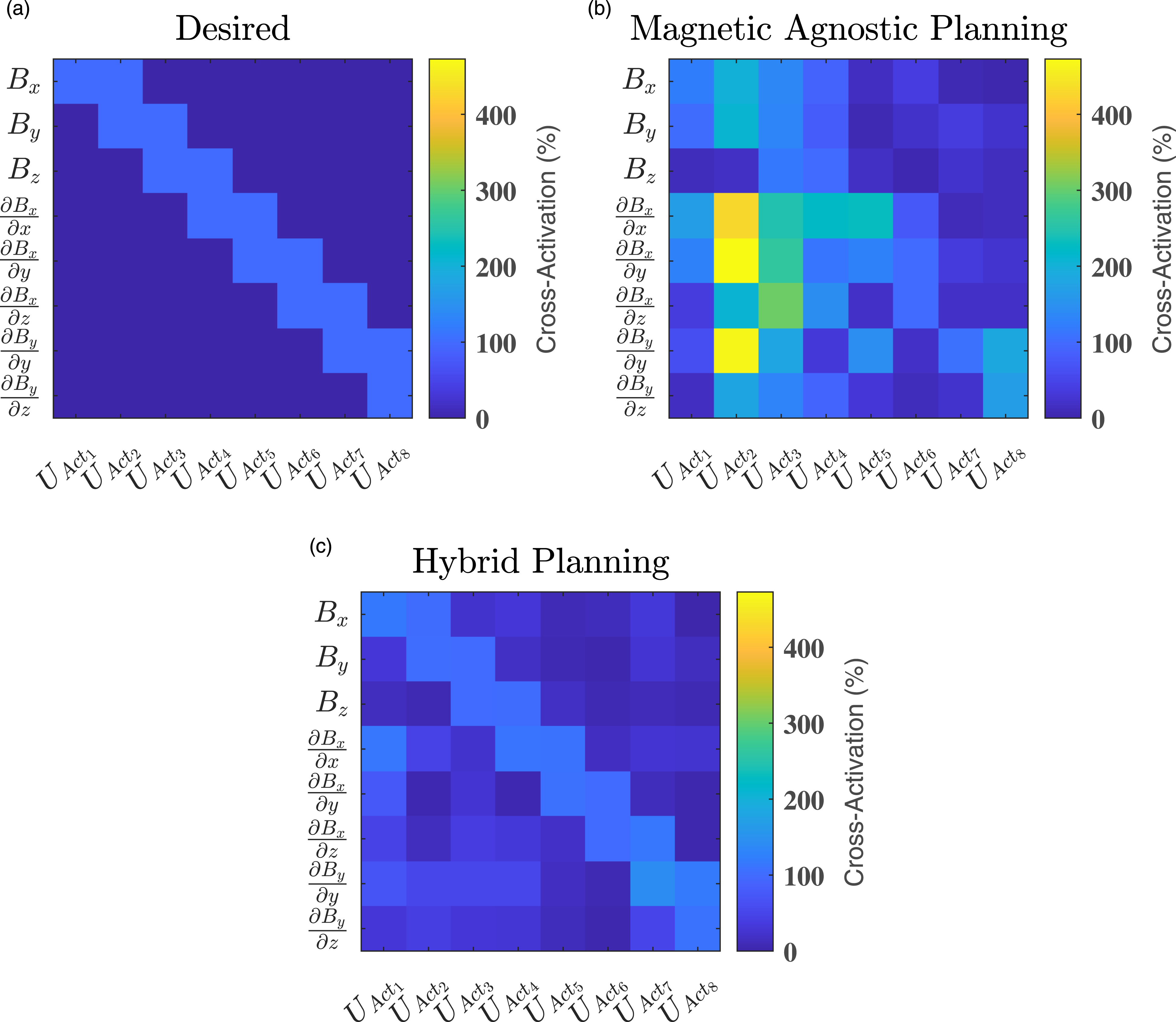
4.3. Discussion: Hybrid planning approach
In order for the dEPM platform to become a feasible source of actuation in healthcare, effective path planning algorithms will be necessary, in particular, for the actuation of multiple magnetic fields and gradients in succession while having a deterministic change in magnetic field. The importance of this stems from the fact that, particularly in the medical field, the device’s movements need to be carried out in a precise manner – any undesired actuation may have potentially harmful results. The algorithm presented in this paper aims to improve robustness and repeatability for magnetically actuated robotic interventions.
This is non-intuitive when using EPMs, due to the highly non-linear relationship between the EPMs’ position and the change of magnetic field. The efficiency of the presented algorithm can be expressed in Big O notation as O(n), where n is the number of waypoints. Therefore, the run-time of the hybrid planner is linearly dependent on the number of waypoints. This method is often considered to be the gold standard for performance approximation of an algorithm in terms of the size of the input.
Figure 5 demonstrates how with the presented path planner different magnetic fields and gradients can be actuated successively with minimal undesired actuation. The difference between actuation using the proposed planner compared to classical EPM based actuation techniques is highlighted by Figure 6. It is also important to note that for these experiments, the final EPM pose related to the actuation of each field or gradient at steady state is the same for the planning and no planning case. The path planning algorithm finds a suitable EPM path which reduces undesired actuation while preventing any collisions.
Our trajectory planning algorithm features two key improvements for managing the operation of magnetically actuated SCR. First, it allows seamless, collision-free, consecutive actuation of fields and gradients, eliminating the need to manually reposition the EPMs to a safe pose between individual actuation steps. Second, despite not completely eliminating undesired actuation, our algorithm minimizes unwanted actuation spikes (shown in Figure 5) which, if unrestricted, could cause notable discrepancies in the movement of a SCR.
The steady state errors highlighted in Table 1 are due to calibration errors in the optical tracking system which reports the position of the magnetic sensors relative to the EPMs. These errors could be reduced through the introduction of a closed loop controller between the magnetic field and gradient generated and the position of the EPMs. The variations in rise and fall phase lags in Figure 5 stem from the requirement for the EPMs to cover differing distances during the actuation of each magnetic field and gradient. Ensuring greater uniformity in the rise and fall times represents a significant focus for the continued development of this algorithm. The use of the trajectory planner significantly reduced the peak off-activation levels, as well as the overshoot during the rise and fall times. These errors were not completely eliminated however with remaining errors attributed to the joint generation section of the proposed trajectory planner. Here, the optimal EPM poses could leave the robotic manipulators in singular positions so slight variations were noted from the expected results.
5. Case study 1: Single-segment SCR
A significant proportion of magnetically actuated SCRs typically consist of a single magnetic section with uniform magnetization (da Veiga et al., 2020). Here, we demonstrate the efficacy of our dEPM planning approach for actuation of an axially magnetized single-segment SCR. The experiment (Supporting Video 2) shows the the precise positioning of the tip of the SCR at four locations, and closely emulates the path taken by a SCR embedded with a laser fibre when ablating a tumour, as previously demonstrated by Kim et al. (2019).
5.1. Single-segment SCR fabrication
For this experiment, we used a cylindrical SCR assembled of two sections; a magnetic tip of length 20 mm and diameter 2 mm, and a silicone overmold (that encapsulates the magnetic tip) of length 70 mm and diameter 2.5 mm. The fabrication process of this SCR is as follows. First, neodymium-iron-boron (NdFeB) micro particles (5 µm diameter, MQFP-B+, Magnequench GmbH, Germany) were mixed with a silicone-based elastomer (Dragon SkinTM 30, Smooth-On, Inc., USA) in a 1.5:1 mass ratio. The mixture was degassed and mixed in a high vacuum mixer (ARV-310, THINKYMIXER, Japan) at 1400 r/min, 20.0 kPa for 90 s. The degassed material was injection molded into a 3D printed (Tough PLA, Ultimaker S5, USA) 20 mm length, 2 mm diameter cylindrical mold, to make the magnetic tip segment. This was cured in a UV oven for 30 min at 40°C (Form Cure, Formlabs, USA). The cured magnetic agent was then magnetized axially by subjecting it to a uniform saturating magnetic field of 4.644 T (ASCIM-10-30, ASC Scientific, USA). The now magnetized tip was placed into the full 70 mm length, 2.5 mm diameter 3D printed cylindrical overmold. The magnetic tip was held at the distal end of the mold using two, 0.2 mm diameter nitinol (NiTi) wire pieces as shown in Figure 7(a). Silicone was mixed with red silicone die (Silc PigTM, PMS 186C, Smooth-On, Inc., USA), with a 1% by weight die-to-silicone ratio. The previous mixing and degassing procedure was repeated before injecting silicone mixture into the 3D printed mold. The injected mold was cured in a UV oven for 30 min at 40°C. The mechanical and elastic properties of the single-segment SCR can be characterized as follows. The magnetic tip has an estimated magnetization vector of 145 kA/m (da Veiga et al., 2021) while the silicone overmold has a linear Elastic Modulus of 593 kPa (Ranzani et al., 2015). We then attached three, 3 mm optical markers (OptiTrack, NaturalPoint, Inc., USA) to the cured SCR using a fast-bonding, high-strength, instant adhesive, to produce the single-segment magnetic SCR shown in Figure 7(b). (a) Fabrication of the single-segment SCR. The magnetic tip was held in place with two pieces of NiTi wire whilst a silicone based elastomer (shown in red) was injected into the closed 3D printed mold. (b) Final single-segement SCR after curing. The magnetic tip was facing downwards such that its magnetization is equal to 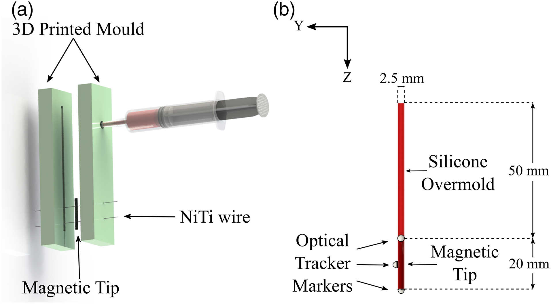
5.2. Experimental setup
With the single-segment SCR hanging vertically as shown in Figure 7(b) and in Supporting Video 2, the norm of the magnetic moment can be described as
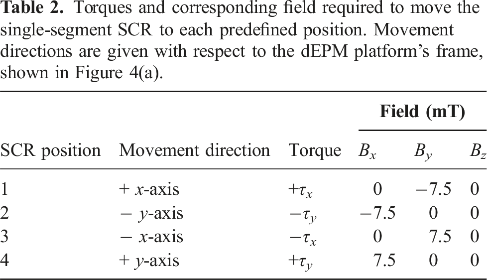
Knowing the magnetic moment of the SCR, the magnetic fields required to produce the desired deflection direction could be calculated using (7). The demonstration chosen for this experiment required the SCR to reach four spots as shown in Figure 8, following the points in the order 0,1, 2, 3, 4, 1, with position 0 being the start position. The magnetic field required for the tip of the SCR to reach each point is found in Table 2. Once the desired field combination had been derived, the dEPM platform was tasked with producing the required fields. This was first done by calculating the required poses as described by Pittiglio et al. (2023), then again using the trajectory planning algorithm, described in Section 3 with 10 waypoints between each desired SCR position. Tip position of a single-segment magnetic SCR in response to the same magnetic fields (a) using the default magnetic agnostic planning (without path planning) and (b) with the hybrid path planner. The tip position measured using the OptiTrack system represented as a coloured line. The colour bar on the right of each figure relates the change in colour to time. Goal points are shown as red dots, and the boundary zone is shown as a black dashed line. Despite using the same desired sequence of magnetic fields in both experiments, the goal points reached in each experiment differ slightly. This is due to undesired torsion in the SCR due to path taken when not using the trajectory planner. A comparison of the different paths taken in the two experiments can be seen in Supplemental Video 2. Torques and corresponding field required to move the single-segment SCR to each predefined position. Movement directions are given with respect to the dEPM platform’s frame, shown in Figure 4(a).
5.3. Results
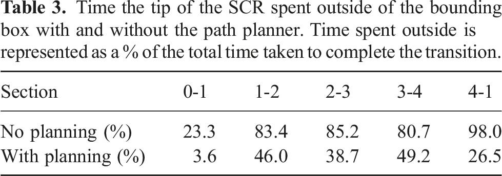
Time the tip of the SCR spent outside of the bounding box with and without the path planner. Time spent outside is represented as a % of the total time taken to complete the transition.
5.4. Discussion
This experiment highlights the difference between planned magnetic actuation and an arbitrary magnetic transition. The path planner, as observed in Figure 8, helped SCR maintain accurate paths and minimized its tendency to deviate from the estimated trajectory. The data strongly suggests the effectiveness of the path planner in controlling and modulating the SCR’s movement, by reducing the time spent outside the predefined area from 74.1% to 32.8%. This is a key feature that can significantly enhance the accuracy and safety of such robots in medical applications such as tumour ablation procedures, where precision and control are paramount. The present algorithm aims to be a first step in the accurate, closed loop control of SCRs’s motion.
The trajectories of the SCR, as illustrated in Figure 8, demonstrate a stark contrast in the path taken. Without the trajectory planner, the SCR was affected by torsion, resulting in a substantial deviation from the planned route and potentially posing a risk in sensitive medical procedures. However, with the trajectory planner, the SCR’s movements were significantly more concise and predictable. Methods to compensate for torsion of SCR when using EPM based actuation without planning have been proposed. These techniques typically require the insertion of a stiffer material through the centre of the SCR (Lloyd et al., 2022) or alter the mechanical design of the SCR (Koszowska et al., 2023) to compensate for torsion in specific directions. This can result in an overall increase in stiffness or diameter of the SCR. In addition, these methods try to eliminate rotation of the SCR around its own axis as a possible DOF. Removing this DOF reduces the possible applications for which SCR could be used, for example, the use of an ultrasound probe where rotation around the long axis may be necessary. The use of the proposed trajectory planning algorithm presents the opportunity to reduce the undesired torsion during magnetic steering of SCRs whilst still maintaining flexibility about this DOF.
6. Case study 2: Navigation of a multi-segment SCR in a soft brain phantom
The capability of independently actuating eight magnetic DOFs, coupled with a non-uniform magnetization profile, allows for the control of multiple points of a magnetic SCR. An example would be a two-segment SCR with orthogonally magnetized segments. Here, we assume that the two magnetic segments are sufficiently close that the local field experienced by each segment can be assumed to be equal. This two segment control enables lengthwise shape forming of the SCR rather than control of the robot’s tip alone. The trajectory planner presented in this paper is applicable to any form of EPMs based actuation. Therefore, we demonstrate the navigational capability of a multi-segment magnetic SCR, actuated using the dEPM platform incorporating the proposed planner. We demonstrate navigation through a complex environment, in this case, a soft phantom of a sample of the vasculature of the brain.
6.1. Soft brain phantom
To demonstrate the enhanced navigational ability of the path planner, a soft brain phantom was manufactured using volumetric Computed Tomography Angiographic (CTA) data from a 47-year-old female with cerebrovascular aneurysms. A segment of the CTA data starting from the middle cerebral artery (MCA) up until the internal carotid artery (ICA) containing terminal ICA aneurysm was selected (Figure 9). The chosen segment of the CTA data was 3D printed (Tough V5 resin, Formlabs II, USA), suspended in a 90 mm by 65 mm acrylic box and then cast in silicone (EcoflexTM Gel, Smooth-On, Inc., USA). This material was chosen due to its Shore hardness of 000-35 closely resembling the bulk behaviour of the brain tissue (Navarro-Lozoya et al., 2019). The silicone was mixed with cure retarder (SLO-JOTM, Smooth-On, Inc., USA) with a ratio of 5% by weight then placed within a vacuum chamber (Renishaw 5/01 vario vacuum casting machine, Renishaw, United Kingdom) to remove any air bubbles. This was cured at 40°C for 40 min (Genlab Prime, Genlab, United Kingdom). On removal, we had a clear, soft and hollow brain phantom of the cerebral vasculature containing an aneurysm as shown in Figure 9. Optical tracking markers were attached to the base of the acrylic box to aid in the calibration of the dEPM platform. Section of the human brain starting from the middle cerebral artery (MCA) to the internal carotid artery (ICA) containing an aneurysm. Each path of the 3D navigation is shown in a different colour. Seen from the (a) side and (b) top. (c) Multi-segment SCR with orthogonally magnetized segments made for navigation of the soft brain phantom.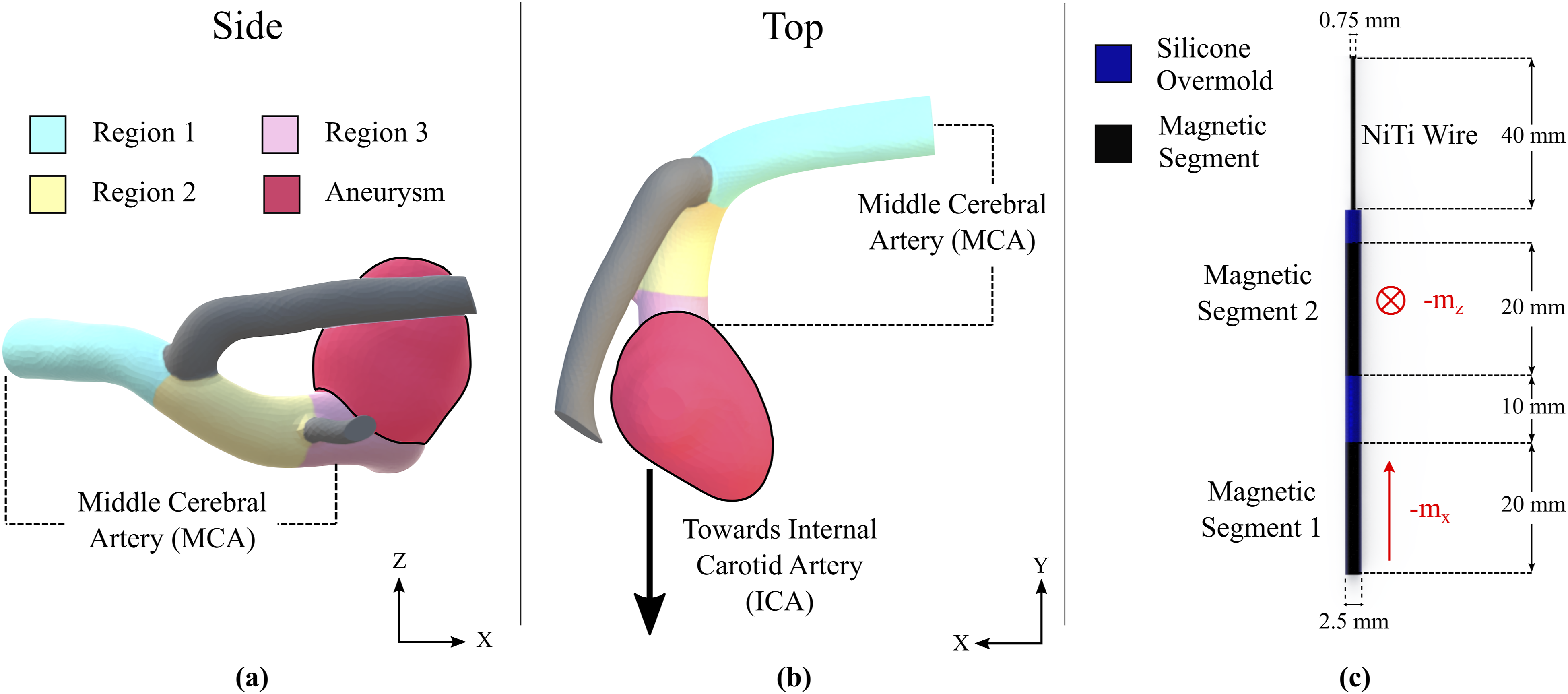
6.2. Multi-segment SCR fabrication
The SCR used in this demonstration is a cylinder of length 50 mm and diameter 2.5 mm containing two magnetic sections with orthogonal magnetic moments. Each magnetic segment is 20 mm long with a separation of 10 mm between each segment. Fabrication was as described in Section 5.1 until the cured magnetic segments were magnetized, with segment 1 magnetized axially, thus having magnetization −
To enable insertion of the SCR into the soft brain phantom, a 40 mm long, 0.75 mm diameter Nitinol wire was attached to the SCR. The base of the Nitinol wire was attached to a Bowden cable passing through a mechanical introducer (Hybrid Stepper Motor MT-1703HSM168RE, MOTECH MOTOR Co. LTD, China). This was used to introduce the SCR into the brain phantom at a speed of 1 mm/s. The final multi-segment SCR can be seen in Figure 9(c).
6.3. Experimental setup
Magnetic wrench applied to each segment of the multi-segment SCR to navigate the soft brain phantom along with the required field and gradient needed to generate the required wrench. Undesired wrenches are shown in bold. The magnitude of the fields and gradients generated by the dEPM at r o are shown in the last column, with fields in mT and gradients in mT/m.
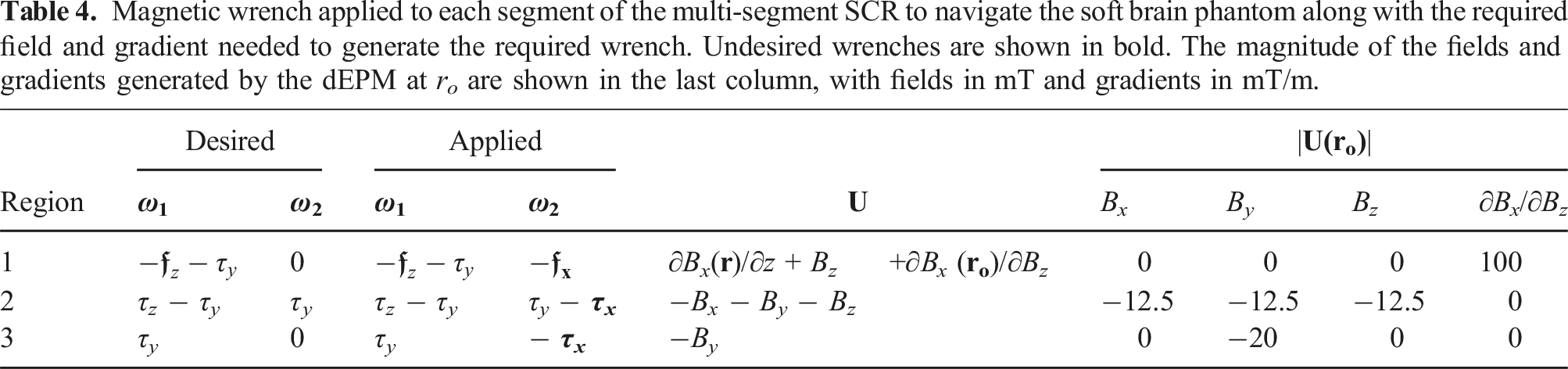
Table 4 shows how some undesired wrenches (shown in bold) are applied during navigation. In path 1, undesired force in the negative x-direction is applied on segment 2; however, this force is countered by the mechanical introducer. In paths 2 and 3, undesired negative torques around the x-axis are applied to the segment 2. This can result in undesirable twisting of the SCR. A point discussed in Section 5.4.
6.4. Results
The first demonstration of this section involved inserting the multi-segment SCR into the soft brain phantom without any magnetic actuation as shown in Supplemental Video 3. Despite the inherent flexibility and softness of the SCR, when no magnetic fields are applied, the SCR collides with the walls of the phantom and starts to deform the structures within the phantom as well as buckling on itself.
Using the magnetic fields and gradients in Table 4 along with the trajectory planner (as shown in Supplemental Video 3) the multi-segment SCR was successfully navigated through the brain phantom to the base of the aneurysm. Figure 10 shows the progression of the SCR through each section of the 3D navigation. Time series showing the multi-segment magnetic SCR’s navigation into the soft brain phantom from three different angles. Using the presented trajectory planner, the SCR (in blue) can be seen to start at the MCA (t = 59 s), navigate through the 3D soft phantom and arrive at the base of the aneurysm (t = 132 s), replicating the path taken by a microcatheter-delivered stent during conventional surgery. Without the use of the trajectory planner, the EPMs collided with the phantom setup. The full 3D navigation with and without the use of the trajectory planner can be seen in Supplemental Video 3.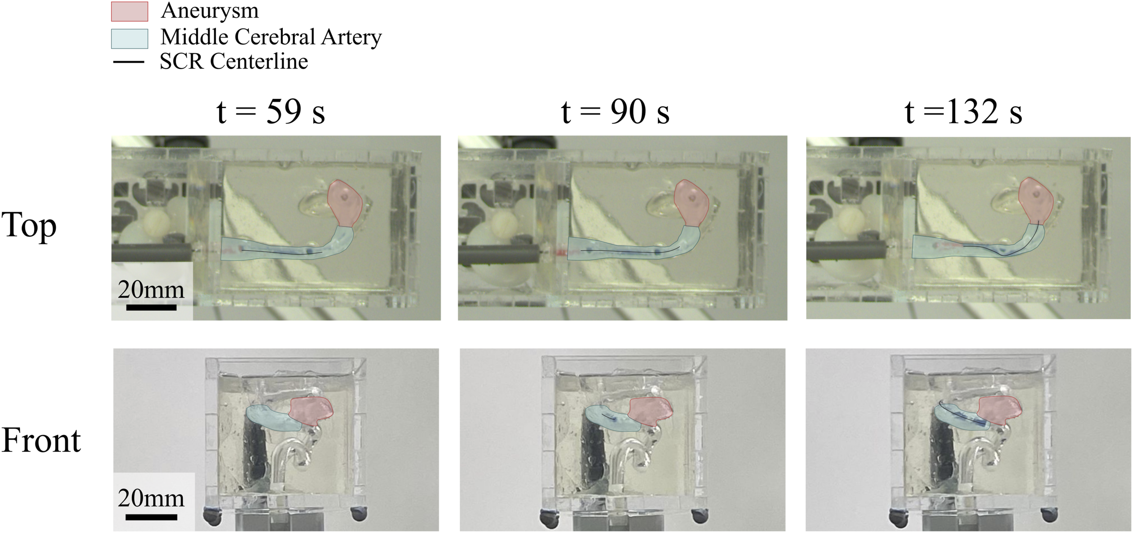
In order to successfully perform the navigation without the use of the trajectory planner (as per the convention developed in Pittiglio et al. (2022)), the EPMs were moved to known ‘zero’ positions between each actuation phase to avoid collisions. Movement to zero positions is not intuitive and often still requires manual planning. This point is highlighted by Supplemental Video 3 where the EPMs inadvertently collided with the phantom, necessitating the activation of the emergency stop button. This shows how the use of the proposed planner will be vital in the safe automation of magnetic SCRs for any practical, medical use.
6.5. Discussion
The rupture of cerebral aneurysms that form along the major arteries within the brain are responsible for approximately 5%–15% of stroke cases (Brisman et al., 2006). Unprompted rupture of intracranial aneurysms typically leads to subarachnoid hemorrhage. This is a subtype of hemorrhagic stroke with a high mortality rate. Even when non-fatal, the reduction in quality of life associated with subarachnoid hemorrhage remains a cause of physical, psychological, and financial damage in both developing and developed nations (Chen et al., 2014). One potential solution to re-rupture of aneurysms is endovascular coiling, where microcatheter-delivered coils are deployed into the aneurysm, with the aim of blocking the blood flow to the aneurysm (Brisman et al., 2006). The coiling mechanism can be stored within the body of the SCR and then be deployed once the navigation process is complete. Alternatively, a magnetic SCR be used as a magnetic guide-wire to navigate standard microcatheter to a position where such coils could deployed, as described by Kim et al. (2022).
Navigating delicate and tortuous pathways such as those in the brain, with minimal rates of error, necessitates more comprehensive shape control than mere tip control. Control of multiple points along the SCR’s body mitigates potentially painful and damaging contact and deformation along the pathway. This is particularly true when operating in the brain. Here, rupture of any blood vessels can cause hemorrhage which can be potentially fatal. The demonstration presented in this paper illustrates how a trajectory planner that considers both magnetic and Cartesian space-based obstacles can assist in such an environment. The ability to navigate 3D pathways with such precision opens up the possibility to introduce magnetically guided solutions for the treatment of intracranial aneurysms.
7. Conclusions and future work
A trajectory planning algorithm has been developed and implemented on the dEPM platform. The same trajectory planning algorithm could be applied to similar robotically actuated EPM systems with minor adjustments, such as altering the kinematic constraints for the particular manipulator used. This algorithm allows for collision-free operation of two robotically actuated permanent magnets, as well as providing a smooth transition through time variant magnetic fields and gradients.
Experimental deployment of the planner revealed high efficacy, acting on each of the eight magnetic DOFs sequentially to avoid potential collisions, the planner reduced the peak off-activation value by an average of 7.3 mT for fields and by a significant 308 mT/m for gradients relative to the absence of path planning.
To further re-enforce the values of the proposed algorithm in a medical context two case studies were carried out. First, the impact of the planned magnetic fields on the actuation of a SCR was analyzed. Second, a single-segment magnetic SCR was assigned to move towards specific points whilst staying within a prescribed boundary. The proposed planner improved the control on movement of the SCR in the restricted area by an average rate of 41.3%. This is particularly significant where precision is paramount, such as in various surgical procedures. In our final experiment, we demonstrated the medical significance of the proposed path planner by guiding a multi-magnetic segment SCR inside a silicone brain phantom. The results show its effectiveness in the control and navigation of the multi-segment SCR, particularly through such complex environments. This underscores the potential of planned magnetic actuation in steering soft robots without causing collateral damage or deformation of surrounding structures.
This work contributes to the advancement of SCR control, setting a foundation for its automation and broadening its applications in the medical field where precision and safety are crucial. Precise control of a SCR would call for a control system that encompasses both the SCR’s physical properties and the proposed trajectory planning algorithm. The development of this controller extends beyond the boundaries of this study and is earmarked for future work. Future studies could also further enhance this planning algorithm, potentially expanding its application across a broader range of scenarios and systems. The same principles used for the algorithm presented could be scaled for systems with more than two EPMs. Here, the same algorithm may be used with slight adjustments to accommodate a greater number of EPMs and other alterations to the workspace. A further improvement could include adapting the planner to consider mobile obstacles and obstacles not in the centre of the workspace. This would be achieved by dynamically altering the planned route. Once the complexity of the system has been increased, the presented algorithm could be altered to no longer be strictly confined to a spherical shape. Finally, it would be highly desirable to incorporate the planned magnetic actuation into a closed loop shape control algorithm, such as that proposed by Edelmann et al. (2017), modified for multi-segment magnetically actuated SCRs with non-uniform magnetization profiles.
Supplemental Material
Supplemental Material
Supplemental Material
Footnotes
Author’s note
Acknowledgements
Special thanks to Mr Samwise Wilson and Dr Dominic Jones for help with experimental arrangements, along with the rest of STORM Lab UK.
Declaration of conflicting interests
The author(s) declared no potential conflicts of interest with respect to the research, authorship, and/or publication of this article.
Funding
The author(s) disclosed receipt of the following financial support for the research, authorship, and/or publication of this article: Research reported in this article was supported by the European Research Council (ERC) under the European Union’s Horizon 2020 research and innovation programme (grant agreement No. 818045), by the Engineering and Physical Sciences Research Council (EPSRC) under grant numbers EP/R045291/1, EP/V009818/1 and EP/S009000/1, and by the National Institute for Health and Care Research (NIHR) Leeds Biomedical Research Centre (BRC) (NIHR203331). The views expressed are those of the authors and not necessarily those of the ERC, EPSRC, NIHR or the Department of Health and Social Care.
ORCID iDs
Supplemental Material
Supplemental material for this article is available online.
References
Supplementary Material
Please find the following supplemental material available below.
For Open Access articles published under a Creative Commons License, all supplemental material carries the same license as the article it is associated with.
For non-Open Access articles published, all supplemental material carries a non-exclusive license, and permission requests for re-use of supplemental material or any part of supplemental material shall be sent directly to the copyright owner as specified in the copyright notice associated with the article.