Optimal potential shaping on SE(3) via neural ordinary differential equations on Lie groups

Abstract

This work presents a novel approach for the optimization of dynamic systems on finite-dimensional Lie groups. We rephrase dynamic systems as so-called neural ordinary differential equations (neural ODEs), and formulate the optimization problem on Lie groups. A gradient descent optimization algorithm is presented to tackle the optimization numerically. Our algorithm is scalable, and applicable to any finite-dimensional Lie group, including matrix Lie groups. By representing the system at the Lie algebra level, we reduce the computational cost of the gradient computation. In an extensive example, optimal potential energy shaping for control of a rigid body is treated. The optimal control problem is phrased as an optimization of a neural ODE on the Lie group SE(3), and the controller is iteratively optimized. The final controller is validated on a state-regulation task.

1. Introduction

Many physical systems are naturally described by the action of Lie groups on their configuration manifolds. This can range from finite-dimensional systems such as rigid bodies, where poses are acted on by the special Euclidean group SE(3) (Murray et al., 1994), towards infinite-dimensional systems such as flexible bodies or fluid dynamical systems, where the diffeomorphism group acts on the configuration of the continuum (Schmid, 2010).

Geometric control systems on Lie groups (Brockett, 1973; Jurdjevic, 1996) exploit the Lie group structure of the underlying physical systems to provide numerical advantages (Marsden and Ratiu, 1999). For example, PD controllers for rigid bodies were defined on SO(3) and SE(3) by Bullo and Murray (1995), and more recently geometric controllers were applied in the context of UAV’s (Goodarzi et al., 2013; Lee et al., 2010; Rashad et al., 2019). Examples for efficient optimal control formulations on Lie groups include linear (Ayala et al., 2021) and nonlinear systems (Spindler, 1998), as well as efficient numerical optimization methods (Kobilarov and Marsden, 2011; Saccon et al., 2013; Teng et al., 2022).

In an orthogonal development over the recent years, there has been a surge of machine learning applications in control (Dev et al., 2021) and robotics (Ibarz et al., 2021; Soori et al., 2023; Taylor et al., 2021). This surge is driven by the need for controllers that work in high-dimensional robotic systems and approximate complex decision policies that require the use of data. The implementation of such controllers through classical control theoretic approaches is prohibitive, and it led to a paradigm shift towards data-driven control (Taylor et al., 2021). Examples of machine learning within high-dimensional systems extend to soft robotics (Kim et al., 2021) and control of fluid systems (Paris et al., 2021). The literature also aims to address common concerns of safety (Brunke et al., 2022; Hewing et al., 2020) both during the training process and in the deployment of systems with machine learning in the loop.

The so-called Erlangen program of machine learning by Bronstein et al. (2021) stresses the importance of geometric machine learning methods: symmetries of data sets can restrict the complexity of functions that are to be learned on them, and thus increase the numerical efficiency of learning frameworks. This rationale also led to extensions of machine learning approaches to Lie groups (Fanzhang et al., 2019; Lu and Li, 2020), with recent applications by Huang et al. (2017); Chen et al. (2021); Forestano et al. (2023).

Indeed, the fundamental symmetry groups in robotics are naturally represented by Lie groups (Marsden and Ratiu, 1999). As such, Lie group-based learning methods are of interest to the robotics community. In an excellent example of a control application Duong and Atanasov (2021b) extended neural ODEs to SE(3) and applied it to the adaptive control of a UAV in Duong and Atanasov (2021a). In their recent work Duong et al. (2024) also highlight the practical use of neural ODEs on Lie groups.

However, a general approach for geometric machine learning in the context of dynamic systems on Lie groups is missing. We believe that such an approach would be of high interest, especially for control applications. In this paper, we address this issue by formalizing neural ODEs on Lie groups.

Our contributions are

1. the formulation of neural ODEs on any finite-dimensional Lie group, with a particular focus on matrix Lie groups;

2. computational simplifications with respect to manifold neural ODEs through use of a compact equation to compute gradients on Lie groups, and reduced dimension with respect to non-intrinsic approaches on Lie groups

3. a pytorch & torchdyn compatible algorithm for the optimization of a general potential energy shaping and damping injection control on SE(3), for which stability is implemented as a design requirement; available at github.com/YPWotte/Lie_nODEs.

4. the formulation of a minimal exponential Atlas on the Lie group SE(3).

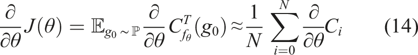
The article is divided into two parts (see also Figure 1): first the formulation of neural ODEs on finite-dimensional matrix Lie groups, and second an extensive example of optimal potential energy shaping on SE(3).

Figure 1.

Overview of the main contribution and structure of the article. Given a parameterized dynamical system on a Lie group, the generalized adjoint method on Lie groups lets us compute the parameter gradient of a cost-functional over system trajectories by solving a set of differential equations. This parameter gradient can then be used to iteratively update parameters by gradient descent. In practice, we sample multiple initial conditions and approximate the parameter gradient of the expected cost 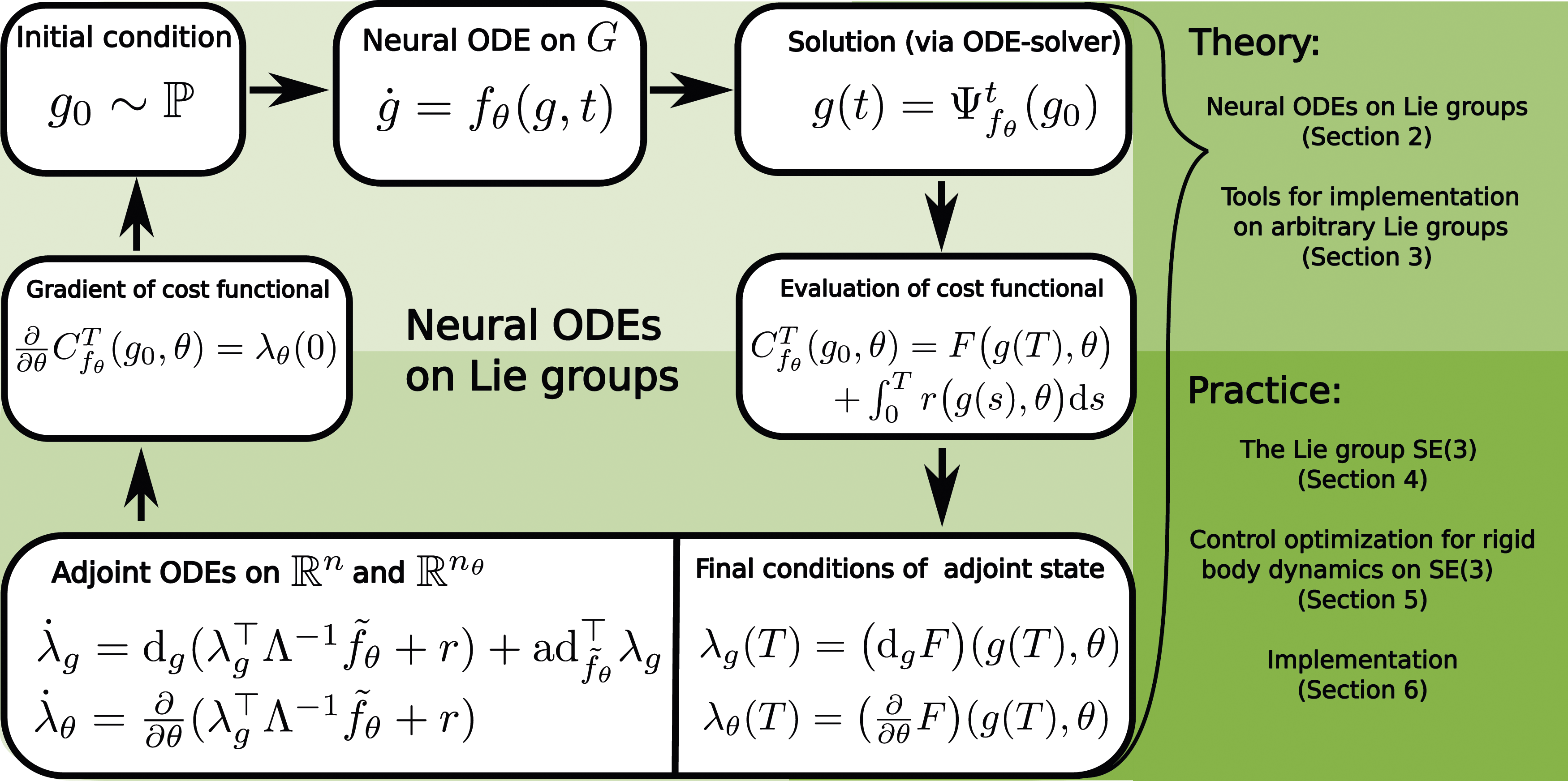$C_{f_{\theta }}^T\left(\theta \right):={\mathbb{E}}_{g_0\mathbb{\sim }\mathbb{P}}{C}_{f_{\theta }}^T\left(g_0,\theta \right)$ .

Section 2 presents the main technical contribution of the article: the generalized adjoint method on Lie groups, which is at the heart of a gradient descent algorithm for dynamics optimization via neural ODEs on Lie groups.

A number of technical tools are required to apply this algorithm on a given matrix Lie group, which are introduced in Section 3. The exponential Atlas allows to implement a numerical procedure for exact integration on Lie groups, while a compact formula for the gradient of a function on a Lie group reduces complexity of the gradient computation.

Section 4 presents the Lie groups SO(3) and SE(3), and gives concrete examples of the technical tools presented in the previous section. One aspect of this is the formulation of a minimal exponential Atlas on SE(3), which is used to formulate an integration procedure on SE(3). This treatment prepares the stage for control optimization of a rigid body on SE(3).

Section 5 introduces the example of optimizing potential energy and damping injection controllers for rigid bodies on SE(3). The class of controllers is defined and it is shown that it guarantees stability by design. Afterward, the optimization of a cost-functional over the defined class of controllers is derived from the general procedure in Section 2.

Finally, Section 6 provides two examples of optimizing controllers for a rigid body on SE(3). The first example concerns pose control, without gravity, and results are compared to a quadratic controller of the type presented by Rashad et al. (2019). In the second example, the controller’s performance is investigated in the presence of gravity.

The article ends with a discussion in Section 7 and a conclusion in Section 8.

1.1 Neural ODEs and relation to existing works

Neural ODEs were first introduced by Chen et al. (2018), who derived them as the continuous limit of recurrent neural nets, taking inputs on ${\mathbb{R}}^n$ . Their cost-functionals only admitted intermediate and final cost terms, for which they showed that the so-called adjoint method allows a memory-efficient computation of the gradient.

Massaroli et al. (2022) introduced a more general framework of neural ODEs, showing the power of state-augmentation and connections to optimal control, while also showing that the cost-functional can include integral cost terms. To this end, they presented the generalized adjoint method.

There are two highly relevant examples in the recent literature that extend neural ODEs to manifolds. The so-called extrinsic picture is presented by Falorsi and Forré (2020), who show that neural ODEs on a manifold $\mathcal{M}$ can be optimized as classical neural ODEs on an embedding ${\mathbb{R}}^n$ . Given an extension of the manifold neural ODE to ${\mathbb{R}}^n$ , they show that the adjoint method on ${\mathbb{R}}^n$ can be applied for optimization of the manifold neural ODE.

An intrinsic picture is presented by Lou et al. (2020), who show that neural ODEs on a manifold $\mathcal{M}$ can be expressed in local charts on the manifold, where the adjoint method holds locally. They use exponential charts on Riemannian manifolds, and achieve a dimensionality-reduction and geometric exactness with respect to Falorsi et al. Both Falorsi and Forré (2020) and Lou et al. (2020) carefully extend neural ODEs to manifolds, and consider neural ODE on Lie groups to be a sub-class of the presented manifold neural ODEs. With respect to their work, we show how to include integral costs in a generalized adjoint method on manifolds and Lie groups, and show the advantages of considering neural ODEs on Lie groups as a specialized class of algorithms.

An example of neural ODEs to control of robotic systems described on ${\mathbb{R}}^n$ is described in Massaroli et al. (2020), where an IDA-PBC controller is optimized.

Duong and Atanasov (2021a,b) apply neural ODEs to control optimization for a rigid body on SE(3). The work focuses on the formulation of an IDA-PBC controller, uses it for dynamics learning and trajectory tracking, and uses neural ODEs as a tool for this optimization. While the integration procedure used is not geometrically exact and the Lie group constraints are violated, the approach is highly successful. However, Duong et al. do not connect their contribution to geometric machine learning literature such as neural ODEs on manifolds. In recent work Duong et al. (2024), steps are made to extend the extrinsic approach to general matrix Lie groups, however without making full use of the geometric structure given by Lie groups.

With respect to Duong et al. (2024), we present neural ODEs on arbitrary finite-dimensional Lie groups. By extending the intrinsic formulation to Lie groups, our example on SE(3) has a reduced number of dimensions (24 instead of 36), and the use of local charts allows geometrically exact integration.

1.2 Notation

While the main results are accessible with a background of linear algebra and vector calculus, the derivations heavily rely on differential geometry and Lie group theory, see, for example, Isham (1999) and Hall (2015) for a complete introduction, or Solà et al. (2021) for a brief introduction with examples in robotics.

Calligraphic letters $\mathcal{M},\mathcal{N},\mathcal{U},\mathcal{P}$ denote smooth manifolds. Respectively, $T_x\mathcal{M}$ and $T_x^{\ast }\mathcal{M}$ denote the tangent and cotangent space at $x\in \mathcal{M}$ , $T\mathcal{M}$ , and $T^{\ast }\mathcal{M}$ denote the tangent bundle and cotangent bundle of $\mathcal{M}$ , and $\mathrm{\Gamma }\left(T\mathcal{M}\right)$ and $\mathrm{\Gamma }\left(T^{\ast }\mathcal{M}\right)$ are the sets of sections that collect vector fields and co-vector fields over $\mathcal{M}$ . Curves $x:\mathbb{R}\to \mathcal{M}$ are evaluated as x(t), and their tangent-vectors are denoted as $\dot{x}\in T_{x\left(t\right)}\mathcal{M}$ .

Upper case letters G, H denote Lie groups, while lower case letters g, h denote their elements. A lower case e denotes the group identity e ∈ G, an upper case I denotes the identity matrix. The Lie algebra is $\mathfrak{g}$ , and its dual is ${\mathfrak{g}}^{\ast }$ . Letters $\stackrel{\sim }{A},\stackrel{\sim }{B}$ denote vectors in the Lie algebra, while letters A, B denote vectors in ${\mathbb{R}}^n$ .

Furthermore $C^k\left(\mathcal{M},\mathcal{N}\right)$ denotes the set of continuous, k-times differentiable functions between $\mathcal{M}$ and $\mathcal{N}$ . For $\varphi \in C^k\left(\mathcal{M},\mathcal{N}\right)$ , let ${\varphi }_{*}:\mathrm{\Gamma }\left(T\mathcal{M}\right)\to \mathrm{\Gamma }\left(T\mathcal{N}\right)$ and ${\varphi }^{\ast }:\mathrm{\Gamma }\left(T^{\ast }\mathcal{N}\right)\to \mathrm{\Gamma }\left(T^{\ast }\mathcal{M}\right)$ denote the push-forward and pullback, respectively.

For $V\in C^1\left(\mathcal{M},\mathbb{R}\right)$ , let $\mathrm{d}V\in \mathrm{\Gamma }\left(T^{\ast }\mathcal{M}\right)$ denote the gradient co-vector field. When $\mathcal{M}={\mathbb{R}}^k$ , the gradient at $x\in {\mathbb{R}}^k$ is denoted by $\partial V/\partial x\in {\mathbb{R}}^k$ .

When coordinate expressions are concerned, the Einstein summation convention is used, that is, the product of variables with lower and upper indices implies a sum a _i b ⁱ ≔ ∑ _i a _i b ⁱ .

Let $\left(X,D,\mathbb{P}\right)$ denote a probability space with X a topological space, D the Borel σ-algebra and $\mathbb{P}:D\to \left[0,1\right]$ a probability measure. Given a vector space L and a random variable C: X → L, denote by ${\mathbb{E}}_{x\mathbb{\sim }\mathbb{P}}\left(C\right):={\int }_{X}C\left(x\right)\mathrm{d}\mathbb{P}\left(x\right)$ the expectation of C w.r.t. $\mathbb{P}$ .

2. Main result

After a brief introduction to Lie groups in Section 2.1, the optimization problem is introduced on abstract Lie groups in Section 2.2. A gradient descent optimization algorithm is presented in Section 2.3. Our main technical result, the generalized adjoint method on Lie groups, lies at the core of the gradient computation. For the sake of exposition, we present it in the context of matrix Lie groups, and relegate the derivations and the formulation on abstract Lie groups to Appendix A.

2.1 Lie groups

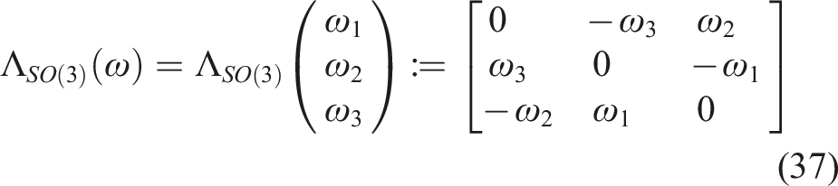
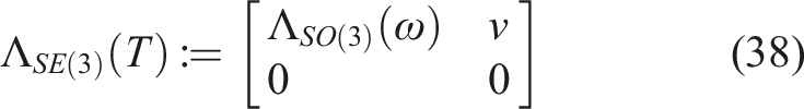
A finite-dimensional Lie group G is an n-dimensional manifold together with a group structure, such that the group operation is a smooth map on G (Isham, 1999). G is a real matrix Lie group if it is a subgroup of the general linear group $GL\left(m,\mathbb{R}\right)$ ¹

$GL\left(m,\mathbb{R}\right):=\left\{g\in {\mathbb{R}}^{m\times m}|\det \left(g\right)\ne 0\right\}$

(1)

where the group operation for a matrix Lie group is given by matrix multiplication (Hall, 2015). For g, h ∈ G the left-translation by h is defined as

$L_h:G\to G;L_h\left(g\right):=hg$

(2)

We denote the Lie algebra of G as $\mathfrak{g}:=T_{e}G$ , and its dual as ${\mathfrak{g}}^{\ast }:=T_e^{\ast }G$ .

Define a basis $E:=\left\{{\stackrel{\sim }{E}}_1,\dots ,{\stackrel{\sim }{E}}_n\right\}$ with ${\stackrel{\sim }{E}}_i\mathfrak{\in }\mathfrak{g}$ , and define the (invertible, linear) map $\mathrm{\Lambda }:{\mathbb{R}}^n\to \mathfrak{g}$ as ²

$\mathrm{\Lambda }:{\mathbb{R}}^n\to \mathfrak{g};\left(x^1,\dots ,x^n\right)\mapsto {\displaystyle \sum }_i{x}^i {\stackrel{\sim }{E}}_i$

(3)

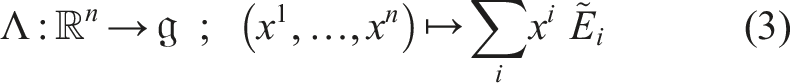
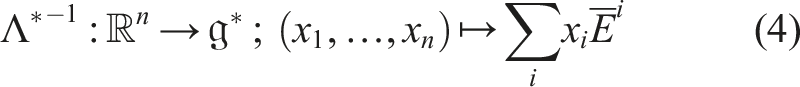
The dual of Λ is the map ${\mathrm{\Lambda }}^{\ast }:{\mathfrak{g}}^{\ast }\to {\mathbb{R}}^n$ . Define the dual basis $\left\{{\overline{E}}^1,\dots ,{\overline{E}}^n\right\}$ with ${\overline{E}}^i\in {\mathfrak{g}}^{\ast }$ by ${\overline{E}}^i\left({\stackrel{\sim }{E}}_j\right)={\delta }_j^i$ with ${\delta }_j^i$ the Kronecker delta. Then ${{\mathrm{\Lambda }}^{\ast }}^{-1}$ is explicitly given by

${{\mathrm{\Lambda }}^{\ast }}^{-1}:{\mathbb{R}}^n\to {\mathfrak{g}}^{\ast };\left(x_1,\dots ,x_n\right)\mapsto {\displaystyle \sum }_i{x}_i{\overline{E}}^i$

(4)

For a matrix Lie group the Lie algebra $\mathfrak{g}$ is a subspace of the Lie algebra $gl\left(m,\mathbb{R}\right)$ of $GL\left(m,\mathbb{R}\right)$ . Here $gl\left(m,\mathbb{R}\right)$ is defined as

$gl\left(m,\mathbb{R}\right):={\mathbb{R}}^{m\times m}$

(5)

For $\stackrel{\sim }{A},\stackrel{\sim }{B}\mathfrak{\in }\mathfrak{g}$ the adjoint map ${\text{ad}}_{\stackrel{\sim }{A}}\left(\stackrel{\sim }{B}\right)$ is a bilinear map defined in terms of the (left) Lie bracket

$\text{ad}:\mathfrak{g}\times \mathfrak{g}\to \mathfrak{g};{\text{ad}}_{\stackrel{\sim }{A}}\left(\stackrel{\sim }{B}\right)=\stackrel{\sim }{A}\stackrel{\sim }{B}- \stackrel{\sim }{B}\stackrel{\sim }{A}$

(6)

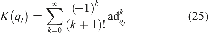
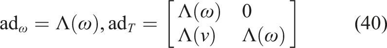
Using the operator Λ, a matrix representation of ad is obtained as ${\mathrm{\Lambda }}^{-1}\left({\text{ad}}_{\mathrm{\Lambda }\left(A\right)}\mathrm{\Lambda }(·)\right)\in {\mathbb{R}}^{n\times n}$ , called the adjoint representation. By an abuse of notation, we denote the adjoint representation as ad _A , without a tilde in the subscript.

On matrix Lie groups and for functions $V\in C^1\left(G,\mathbb{R}\right)$ the gradient ${\mathrm{d}}_{g}V\in {\mathbb{R}}^n$ (see Section 3.4 for details) is found as

${\mathrm{d}}_{g}V=\frac{\partial }{\partial q}V{\left(g\left(I+\mathrm{\Lambda }\left(q\right)\right)\right)}_{|q=0}$

(7)

2.2 Optimization problem

We consider a variant of the optimal control problem on a Lie group (Jurdjevic, 1996) with a finite horizon T. Given parameters $\theta \in {\mathbb{R}}^{n_{\theta }}$ , denote the parameterized dynamics on a Lie group as f _θ (g, t)≔f(g, t, θ). Then, given the dynamic system

$\dot{g}=f_{\theta }\left(g,t\right),g\left(0\right)=g_0$

(8)

denote the solution operator (also called the flow) as

${\mathrm{\Psi }}_{f_{\theta }}^t:G\to G;g\left(0\right)\mapsto g\left(t\right)$

(9)

and define the real valued cost function

$C_{f_{\theta }}^T\left(g_0,\theta \right)=F\left({\mathrm{\Psi }}_{f_{\theta }}^T\left(g_0\right),\theta \right)+{\int }_0^{T}r\left({\mathrm{\Psi }}_{f_{\theta }}^s\left(g_0\right),\theta ,s\right)\mathrm{d}s$

(10)

where we call F the final cost term and r the running cost term.

Indicating a probability space $\left(G,D,\mathbb{P}\right)$ , we are interested in solving the minimization problem

$\underset{\theta }{\min }{\mathbb{E}}_{g_0\mathbb{\sim }\mathbb{P}}{C}_{f_{\theta }}^T\left(g_0,\theta \right)$

(11)

Remark 2.1

The chief reason for our interest in this optimization problem is that it includes, as a sub-class, the optimization of state-feedbacks $u_{\theta }:G\times \left[0,T\right]\to \mathcal{U}$ by considering dynamics of the form f(g, t, u _θ (g, t)), where u _θ denotes the control input of the system.

Remark 2.2

The dynamics f _θ (g, t) can also be parameterized with neural nets, in which case f _θ (g, t) is referred to as a neural ODE on a Lie group. Indeed, for the Lie group $\left({\mathbb{R}}^n,+\right)$ , the formulation agrees with the definition of a neural ODE given in Massaroli et al. (2022) who define them as dynamics $\dot{x}=f_{\theta }\left(x,t\right)\hspace{0.17em}with\hspace{0.17em}x\in {\mathbb{R}}^n$ .

2.3 Optimization algorithm

We use a stochastic gradient descent optimization algorithm (Robbins and Monro, 1951) to approximate a solution to the optimization problem (11) on a matrix Lie group.

Denote the total cost in (11) as

$J\left(\theta \right):={\mathbb{E}}_{g_0\mathbb{\sim }\mathbb{P}}{C}_{f_{\theta }}^T\left(g_0,\theta \right)$

(12)

Additionally, denote by ${\theta }_k\in {\mathbb{R}}^{n_{\theta }}$ the parameters at the k-th iteration, and by η _k a positive scalar learning rate at the k-th iteration. Then a standard gradient descent algorithm computes the parameters θ_k+1 by an application of the update rule

${\theta }_{k+1}={\theta }_k-{\eta }_k\frac{\partial }{\partial \theta }J\left(\theta \right)$

(13)

In stochastic gradient descent N initial conditions g _i are sampled from the probability distribution corresponding to the probability measure $\mathbb{P}$ . The expectation in (13) is approximated by averaging the gradients of costs $C_i=C_{f_{\theta }}^T\left(g_i,\theta \right)$ of the individual trajectories starting at g _i as

$\frac{\partial }{\partial \theta }J\left(\theta \right)={\mathbb{E}}_{g_0\mathbb{\sim }\mathbb{P}}\frac{\partial }{\partial \theta }{C}_{f_{\theta }}^T\left(g_0\right)\approx \frac{1}{N}{\displaystyle \sum }_{i=0}^N\frac{\partial }{\partial \theta }{C}_i$

(14)

For convex cost-functions J(θ) and a sufficiently small η _k , the parameter θ _k approaches the optimal parameters θ^⋆ as k increases (Robbins and Monro, 1951). For non-convex cost-functions stochastic gradient descent does not have a guarantee of global optimality, but it is still widely used as a light and scalable algorithm (Ruder, 2017) that results in robust local optima (Xie et al., 2021).

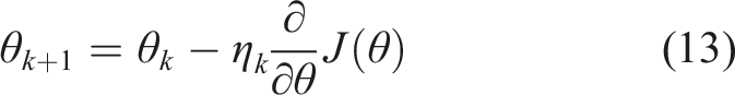
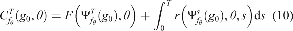
In order to compute the gradient ∂/∂θC _i of the cost for a single trajectory (10), we derived the generalized adjoint method on matrix Lie groups. It is the main technical result of this paper, and it is stated in the following:

Theorem 2.1

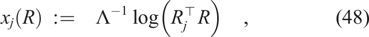
Generalized Adjoint Method on Matrix Lie Groups. Given are the dynamics (8) and the cost (10). Denote by ${\stackrel{\sim }{f}}_{\theta }\left(g,t\right):=g^{-1}{f}_{\theta }\left(g,t\right)\mathfrak{\in }\mathfrak{g}$ . Then the parameter gradient $\partial /\partial \theta C_{f_{\theta }}^T\left(g_0\right)$ of the cost is given by the integral equation

$\frac{\partial }{\partial \theta }{C}_{f_{\theta }}^T\left(g_0\right)=\frac{\partial F}{\partial \theta }+{\int }_0^T\frac{\partial }{\partial \theta }\left({\lambda }_g^{\top }{\mathrm{\Lambda }}^{-1}\left({\stackrel{\sim }{f}}_{\theta }\right)\right)+\frac{\partial r}{\partial \theta }dt$

(15)

where the state g(t) ∈ G and adjoint state ${\lambda }_g\left(t\right)\in {\mathbb{R}}^n$ are the solutions of the system of equations

$\begin{array}{l}\dot{g}=f_{\theta },g\left(0\right)=g_0,\end{array}$

(16)

$\begin{array}{ll}{\stackrel{.}{\lambda }}_g& =-d_g\left({\lambda }_g^{\top }{\mathrm{\Lambda }}^{-1}\left({\stackrel{\sim }{f}}_{\theta }\right)+r\right)+{ad}_{{\stackrel{\sim }{f}}_{\theta }}^{\top }{\lambda }_g,{\lambda }_g\left(T\right)=d_{g}F\end{array}$

(17)

Proof. For a derivation of Theorem 2.1 via neural ODEs on manifolds, refer to Appendix A.

The generalized adjoint method (Massaroli et al., 2022) on ${\mathbb{R}}^n$ is recovered as a special case for the Lie group $\left({\mathbb{R}}^n,+\right)$ , for which the adjoint term ad _T = 0 such that equation (17) agrees with the adjoint equation on ${\mathbb{R}}^n$ .

Just as the generalized adjoint method on ${\mathbb{R}}^n$ , the generalized adjoint method on Lie groups has a constant memory efficiency with respect to the network depth T. This makes it an advantageous choice for the gradient computation compared to, for example, back-propagation through an ODE-solver.

Various technical tools are required to apply Theorem 2.1 in practice. This includes the exponential Atlas for exact integration of $\dot{g}$ , a tractable expression of the gradient operator ${\mathrm{d}}_g:C^1\left(G,\mathbb{R}\right)\to {\mathbb{R}}^n$ , and the composition of matrix Lie groups to create new matrix Lie groups from old ones. These tools are the subject of Section 3.

Remark 2.3

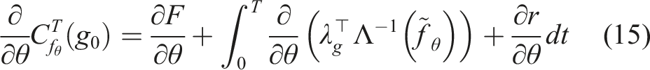
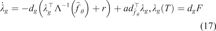
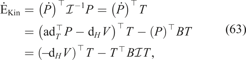
Equations (16) and (17) are solved by integrating (16) forward in time, computing d _g F at g = g(T), and integrating (17) backwards in time, reusing g(t) from the forward integration. Equation (15) is solved by integrating its differential alongside Equation (17). See especially Figure 1. The memory efficiency of neural ODEs stems from the fact that trajectories g(t) and λ _g (t) do not need to be stored, apart from a few way-points of g(t), and that the dependency of g(t) on parameters is largely ignored in the forward pass - this avoids overheads that arise, for example, through automatic differentiation over an ODE-solver.

Remark 2.4

The choice of group action for $\left({\mathbb{R}}^n,•\right)$ plays an important role in recovering the adjoint equation on ${\mathbb{R}}^n$ . This choice is a nontrivial degree of freedom of the optimization (see also Remark 5.3).

3. Technical tools

A number of technical tools are presented in the context of matrix Lie groups. Given mild adaptations of the definitions these tools also apply to abstract finite-dimensional Lie groups (see Appendix A.4).

3.1 Atlas and minimal atlas on Lie groups

In this section the exponential map and logarithmic maps will be used to construct an atlas of exponential charts for finite-dimensional Lie groups, and the concept of a minimal exponential atlas will be defined. Here an atlas is defined as follows:

Definition 3.1

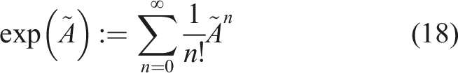
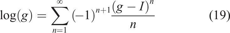
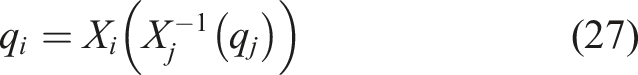
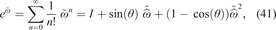
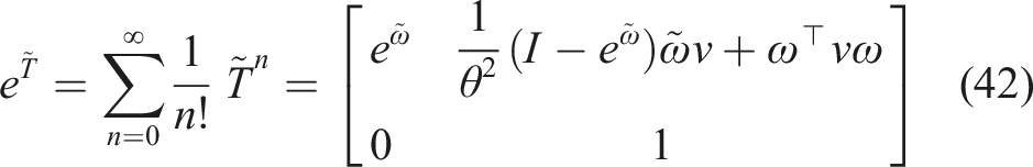
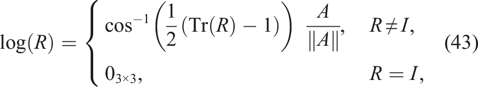
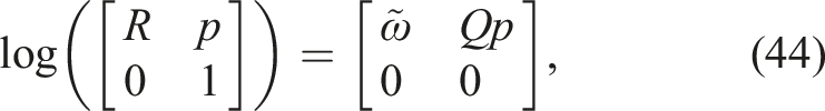
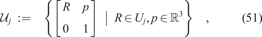
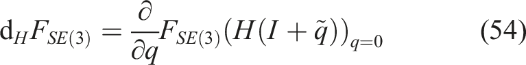
Atlas and Charts. An atlas $\mathcal{A}$ for an n-dimensional smooth manifold $\mathcal{M}$ is a collection of charts (U, X), where $U\subseteq \mathcal{M}\hspace{0.17em}is\hspace{0.17em}an\hspace{0.17em}open\hspace{0.17em}set,X:U\to {\mathbb{R}}^n$ is a diffeomorphism called a chart map , and the chart domains satisfy $\underset{\left(U,X\right)\in \mathcal{A}}{\cup }U=\mathcal{M}$ .

For finite-dimensional Lie groups the exponential map $\exp :\mathfrak{g}\to G$ is a local diffeomorphism (Isham, 1999: Chapter 4.2.3). Its inverse $\log :U\to \mathfrak{g}$ is defined by exp ◦ log  = id _U , for a neighborhood U of the identity e ∈ G, and id _U is the identity map on U.

For a matrix Lie group, the exponential map is given by the infinite sum (Hall, 2015: Chapter 3.7):

$\exp \left(\stackrel{\sim }{A}\right):={\displaystyle \sum }_{n=0}^{\infty }\frac{1}{n!}{\stackrel{\sim }{A}}^n$

(18)

Conversely, the log map for matrix Lie groups is given by the matrix logarithm, when it is well-defined (Hall, 2015: Chapter 2.3):

$\log \left(g\right)={\displaystyle \sum }_{n=1}^{\infty }{\left(-1\right)}^{n+1}\frac{{\left(g-I\right)}^n}{n}$

(19)

On a case-by-case basis the infinite sums in (18) and (19) can further be reduced to a finite sum by use of the Cayley-Hamilton theorem (Visser et al., 2006), which often allows one to find a closed-form expression of the exp and log maps.

The logarithmic map (19) and Λ in equation (3) can then be used to construct a local exponential chart (U, X) for G, where

$X:U\to {\mathbb{R}}^n;g\mapsto {\mathrm{\Lambda }}^{-1}\hspace{0.17em}\log \left(g\right)$

(20)

assigns so-called coordinates $q\in {\mathbb{R}}^n$ to group elements g ∈ U ⊆ G, with the zero coordinates assigned to the group identity e.

To create a chart “centered” on any h ∈ G (i.e., the zero coordinates are assigned to h), both the region U and the chart map X can be left-translated ³ by L _h to define the chart (U _h , X _h ) with

$\begin{array}{l}{U}_h=\left\{hg|g\in U\right\},\end{array}$

(21)

$\begin{array}{l}{X}_h:U_h\to {\mathbb{R}}^n;g\mapsto {\mathrm{\Lambda }}^{-1}\hspace{0.17em}\log \left(h^{-1}g\right),\end{array}$

(22)

$\begin{array}{l}{X}_h^{-1}:{\mathbb{R}}^n\to G;q\mapsto h\hspace{0.17em}\exp \left(\mathrm{\Lambda }\left(q\right)\right)\end{array}$

(23)

The collection $\mathcal{A}$ of charts (U _h , X _h ) is then called an exponential atlas. This atlas covers the Lie group G, and is fully determined by the choice of basis $E\mathfrak{\subset }\mathfrak{g}$ and chart region U ⊂ G.

In order to use a finite number of charts, we are interested in constructing a minimal exponential atlas. A minimal atlas is defined as follows:

Definition 3.2

Minimal Atlas. An atlas $\mathcal{A}$ is minimal if it covers the manifold, that is, $\mathcal{M}=\underset{\left(U,X\right)\in \mathcal{A}}{\cup }U$ , and if it does so with the minimum number of charts.

Remark 3.1

Given a manifold $\mathcal{M}$ , the size of a minimal atlas is determined by a topological invariant, the integer $Cat\left(\mathcal{M}\right)$ (the Lusternik-Schnirrelmann category, see Grafarend and Kühnel (2011); Oprea (2014)). Given a Lie group G, Cat(G) provides a lower bound on the size of a minimal exponential atlas.

Remark 3.2

Given a minimal exponential atlas (which can be seen to be always countable) we use integers j to number the relevant chart-centers as g _j , the corresponding charts as (U _j , X _j ), and denote the chart-coordinates in the j-th chart as $q_j\in {\mathbb{R}}^n$ .

3.2 Vectors on Lie groups

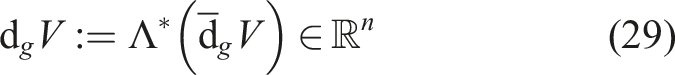
Given a curve $g:\mathbb{R}\to G$ and its coordinate representation q _j (t) = X _j (g(t)) through (22), one can relate the tangent-vector ${\dot{q}}_j\in T_{q_j}{Q}_j$ of $q_j\in Q_j\subseteq {\mathbb{R}}^n$ to an element $\stackrel{\sim }{A}\mathfrak{\in }\mathfrak{g}$ , and further to an element $A={\mathrm{\Lambda }}^{-1}\left(\stackrel{\sim }{A}\right)\in {\mathbb{R}}^n$ (see Figure 2) by

$A=K\left(q_j\right){\dot{q}}_j$

(24)

The map $K:{\mathbb{R}}^n\to {\mathbb{R}}^{n\times n}$ is called the derivative of the exponential map, and it is given by the power series (Rossmann, 2006)

$K\left(q_j\right)={\displaystyle \sum }_{k=0}^{\infty }\frac{{\left(-1\right)}^k}{\left(k+1\right)!}{\text{ad}}_{q_j}^k$

(25)

Figure 2.

Commutative diagram of a generic Lie group G. Boxes represent sets, while arrows represent functions between sets. Relevant variables in a given set are indicated in red.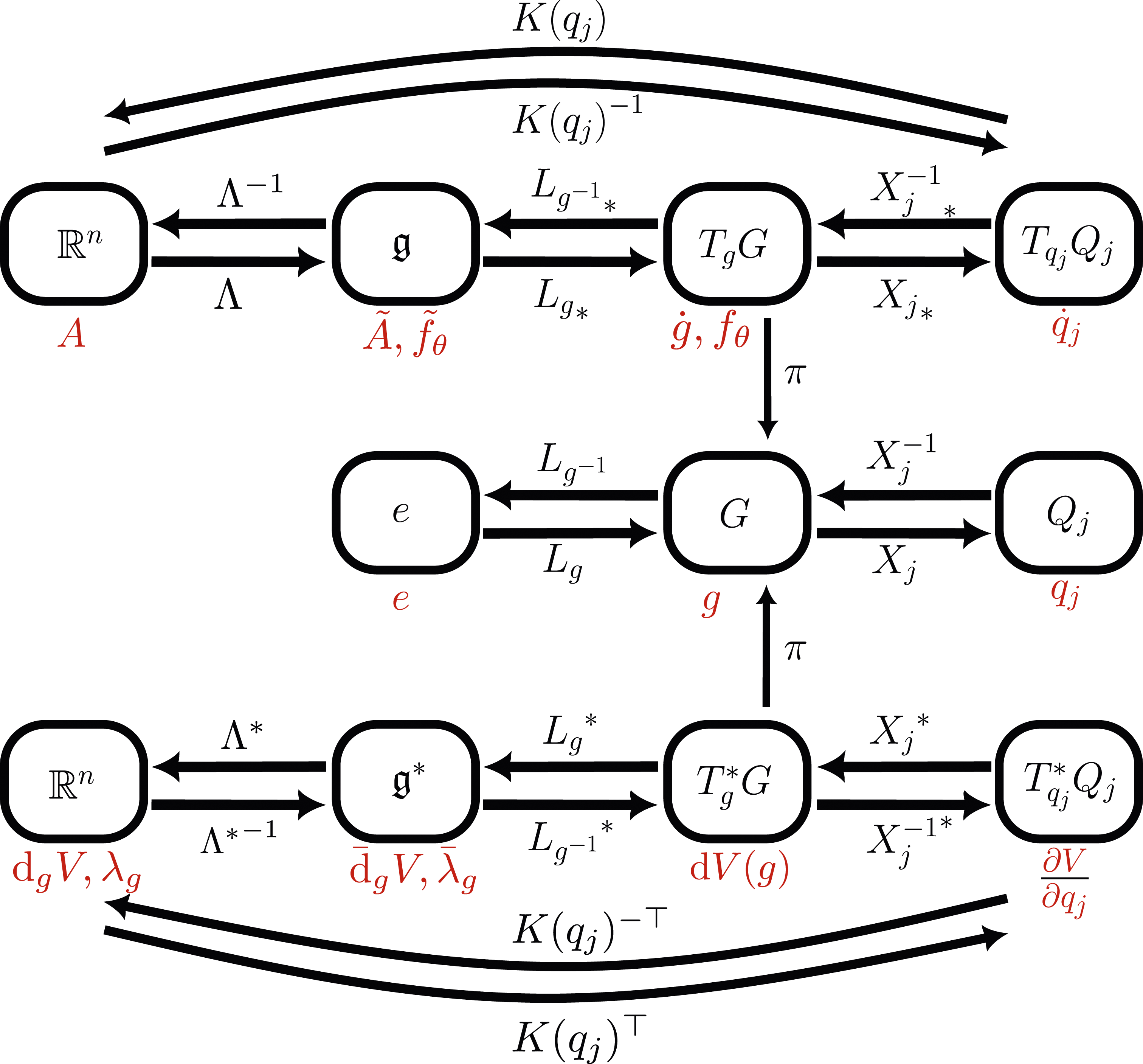

Recall that ${\text{ad}}_{q_j}$ is an n-by-n matrix, and ${\text{ad}}_{q_j}^k$ is the k-th power of such matrices. As with the matrix exponential (18), the infinite sum can then be reduced to a finite sum by use of the Cayley-Hamilton theorem (Visser et al., 2006).

Remark 3.3

The expression (24) is invariant under choice of exponential chart, that is, for any charts (U _j , X _j ) and (U _k , X _k ) one has that $K\left(q_j\right){\dot{q}}_j=K\left(q_k\right){\dot{q}}_k$ (see Appendix B.1).

3.3 Lie group integrators

We adapt the Runge-Kutta-Munthe-Kaas (RKMK) method (Munthe-Kaas, 1999) for exact integration of the dynamics (8). The RKMK method uses the Runge-Kutta scheme on Lie groups—we instead allow for arbitrary numerical integration schemes. For an overview of Lie group integrators, see, for example, Iserles et al. (2000); Celledoni and Owren (2003); Celledoni et al. (2014).

Using equation (24), the dynamics (8) can be represented in a local exponential chart as (Celledoni et al., 2014)

${\dot{q}}_j=K{\left(q_j\right)}^{-1}{\mathrm{\Lambda }}^{-1}{\stackrel{\sim }{f}}_{\theta }\left(X_j^{-1}\left(q_j\right),t\right)$

(26)

where we denote ${\stackrel{\sim }{f}}_{\theta }\left(g,t\right):=g^{-1}{f}_{\theta }\left(g,t\right)\mathfrak{\in }\mathfrak{g}$ . An arbitrary numerical integration scheme can then be used to integrate the dynamics, as long as the state q _j remains in the chart region $Q_j=X_j\left(U_j\right)\subseteq {\mathbb{R}}^n$ .

Remark 3.4

Note that the chart-dynamics (26) are not necessarily well-defined for all $q_j\in {\mathbb{R}}^n$ , since K(q _j ) can have singularities. Yet, the chart-dynamics are well-defined for q _j in the chart region Q _j , where K(q _j ) is guaranteed to be of full rank.

To make sure the state remains within the chart region we switch charts when needed by application of

$q_i=X_i\left(X_j^{-1}\left(q_j\right)\right)$

(27)

Here the conditions for chart switches are a degree of freedom. It is possible to always choose the chart (X _h , U _h ) with $h=X_j^{-1}\left(q_j\left(t\right)\right)$ , that is, to switch charts after every step of the numerical integrator as in Munthe-Kaas (1999); Celledoni et al. (2014).

Given a minimal exponential atlas, we choose to reduce the amount of chart switches. To this end, we introduce indicator functions ${\sigma }_j:G\to \mathbb{R}$ s.t. σ _j (g) > 0 if g ∈ U _j , and switch charts when σ _j (g) is smaller than a threshold-value (see Appendix B.2).

Remark 3.5

The use of a minimal exponential atlas allows to store way-points of a trajectory $g\left(t\right)\in G\subset GL\left(m,\mathbb{R}\right)$ in terms of the n + 1 numbers (q _j (t), j), rather than storing the m × m entries of g. In principle, this more memory-efficient storing does not require an integration procedure based on a minimal atlas, since it can be implemented as a post-processing step given the trajectory g(t). While not done in this work, it is worth consideration to use standard numerical integrators such as RKMK, which come with well-known error-bounds (Munthe-Kaas, 1999).

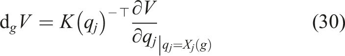
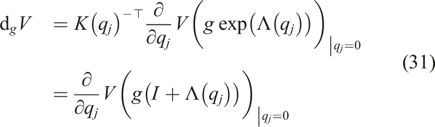
3.4 Gradients on Lie groups

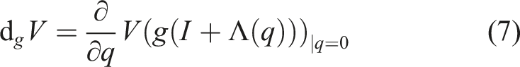
The gradient of a function $V\in C^1\left(G,\mathbb{R}\right)$ is the co-vector field dV ∈ Γ(TG). For any given g ∈ G the gradient $\mathrm{d}V\left(g\right)\in T_g^{\ast }G$ is a co-vector, and transforms in a dual manner to a vector $\dot{g}\in T_{g}G$ . With reference to Figure 2, the gradient can be represented as

${\overline{\mathrm{d}}}_{g}V:={\left(L_g\right)}^{\ast }\mathrm{d}V\left(g\right)\in {\mathfrak{g}}^{\ast }$

(28)

and as

${\mathrm{d}}_{g}V:={\mathrm{\Lambda }}^{\ast }\left({\overline{\mathrm{d}}}_{g}V\right)\in {\mathbb{R}}^n$

(29)

Equivalently, d _g V can be found from the computation in a chart (U _j , X _j ) as (indeed, dual to (24))

${\mathrm{d}}_{g}V=K{\left(q_j\right)}^{-\top }{\frac{\partial V}{\partial q_j}}_{|q_j=X_j\left(g\right)}$

(30)

Here, a computationally advantageous choice can be made for the chart map X _j : by choosing the chart (U _j , X _j ) = (U _g , X _g ) in (21) one finds that K(X _j (g)) = K(0) = I _n , such that the computation of (25) can be avoided:

$\begin{array}{ll}{\mathrm{d}}_{g}V& =K{\left(q_j\right)}^{-\top }\frac{\partial }{\partial q_j}V{\left(g\hspace{0.17em}\exp \left(\mathrm{\Lambda }\left(q_j\right)\right)\right)}_{|q_j=0}\\ & =\frac{\partial }{\partial q_j}V{\left(g\left(I+\mathrm{\Lambda }\left(q_j\right)\right)\right)}_{|q_j=0}\end{array}$

(31)

The final simplification in equation (31) holds for matrix Lie groups, where higher order terms of the power series (18) can be neglected.

3.5 Composition of Lie groups

We briefly review the composition of Lie groups. Lie groups G and H can always be composed to form a product Lie group G × H. For matrix Lie groups $G\subset GL\left(m,\mathbb{R}\right)$ and $H\subset GL\left(l,\mathbb{R}\right)$ , a product Matrix Lie group $G\times H\subset GL\left(m+l,\mathbb{R}\right)$ can be defined as (Hall, 2015, Definition 4.17)

$G\times H:=\left\{\left[\begin{array}{ll}g& 0\\ 0& h\end{array}\right]|g\in G,h\in H\right\}$

(32)

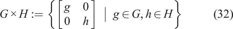
The composition of matrix Lie groups has a block-diagonal structure. This block-diagonal structure reappears in the construction of the corresponding Lie algebra $\mathfrak{g}\mathfrak{\oplus }\mathfrak{h}\mathfrak{\subset }gl\left(m+l,\mathbb{R}\right)$ , the adjoint map, exponential map and the logarithmic map, which consist of their counterparts for G and H. The algebra representation $\mathrm{\Lambda }:{\mathbb{R}}^{n+k}\to \mathfrak{g}\mathfrak{\oplus }\mathfrak{h}$ can likewise be chosen to consist of the components ${\mathrm{\Lambda }}_G:{\mathbb{R}}^n\to \mathfrak{g}$ and ${\mathrm{\Lambda }}_H:{\mathbb{R}}^k\to \mathfrak{h}$ .

4. The cases SO(3) and SE(3)

Prior theory is applied to the Lie groups SO(3) and SE(3).

4.1 The matrix Lie groups SO(3) and SE(3)

Here, the special orthogonal group SO(3) and the special Euclidean group SE(3) are directly defined as matrix Lie groups that collect transformations of the Euclidean 3-space ${\mathbb{R}}^3$ . SO(3) can be described as the collection of rotations of a vector space ${\mathbb{R}}^3$ , and SE(3) as the collection of simultaneous rotations and translations of ${\mathbb{R}}^3$ , implemented on the vector space of homogeneous vectors (vectors of the form $\left(\begin{array}{l}x\\ 1\end{array}\right)$ with $x\in {\mathbb{R}}^3$ , see (Murray et al., 1994, Ch. 3.1)).

Define $SO\left(3\right)\subset GL\left(3,\mathbb{R}\right)$ and $SE\left(3\right)\subset GL\left(4,\mathbb{R}\right)$ as the matrix Lie groups

$\begin{array}{l}SO\left(3\right):=\left\{R\in {\mathbb{R}}^{3\times 3}|R^{\top }R=I,\det \left(R\right)=1\right\},\end{array}$

(33)

$\begin{array}{l}SE\left(3\right):=\left\{\left[\begin{array}{ll}R& p\\ 0& 1\end{array}\right]\in {\mathbb{R}}^{4\times 4}|R\in SO\left(3\right),p\in {\mathbb{R}}^3\right\}\end{array}$

(34)

in both cases using matrix composition as the group operation.

Remark 4.1

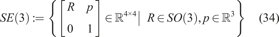
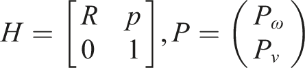
Concerning notation for relative poses of rigid bodies: $H_B^A\in SE\left(3\right)$ indicates the pose of a reference frame Ψ _B as seen from Ψ _A , while $H_A^B={H_B^A}^{-1}$ .

The Lie algebras of SO(3) and SE(3) are the vector spaces $so\left(3\right)\subset gl\left(3,\mathbb{R}\right)$ and $se\left(3\right)\subset gl\left(4,\mathbb{R}\right)$ , respectively, with their Lie bracket given by the matrix commutator. The Lie algebras so(3) and se(3) are given by

$\begin{array}{l}so\left(3\right):=\left\{\stackrel{\sim }{\omega }\in {\mathbb{R}}^{3\times 3}| \stackrel{\sim }{\omega }=-{\stackrel{\sim }{\omega }}^{\top }\right\},\end{array}$

(35)

$\begin{array}{l}se\left(3\right):=\left\{\left[\begin{array}{ll}\stackrel{\sim }{\omega }& v\\ 0& 0\end{array}\right]\in {\mathbb{R}}^{4\times 4}|\stackrel{\sim }{\omega }\in so\left(3\right),v\in {\mathbb{R}}^3\right\}\end{array}$

(36)

Arbitrary elements of so(3) and se(3) will be denoted by $\stackrel{\sim }{\omega }$ and $\stackrel{\sim }{T}$ , respectively.

The vector space isomorphism ${\mathrm{\Lambda }}_{SO\left(3\right)}:{\mathbb{R}}^3\to so\left(3\right)$ is defined as

${\mathrm{\Lambda }}_{SO\left(3\right)}\left(\omega \right)={\mathrm{\Lambda }}_{SO\left(3\right)}\left(\begin{array}{l}{\omega }_1\\ {\omega }_2\\ {\omega }_3\end{array}\right):=\left[\begin{array}{lll}0& -{\omega }_3& {\omega }_2\\ {\omega }_3& 0& -{\omega }_1\\ -{\omega }_2& {\omega }_1& 0\end{array}\right]$

(37)

For SE(3), define ${\mathrm{\Lambda }}_{SE\left(3\right)}:{\mathbb{R}}^6\to se\left(3\right)$ for $T=\left(\begin{array}{l}\omega \\ v\end{array}\right)\in {\mathbb{R}}^6$ with $\omega ,v\in {\mathbb{R}}^3$ , via

${\mathrm{\Lambda }}_{SE\left(3\right)}\left(T\right):=\left[\begin{array}{ll}{\mathrm{\Lambda }}_{SO\left(3\right)}\left(\omega \right)& v\\ 0& 0\end{array}\right]$

(38)

Both Λ_SO(3) and Λ_SE(3) will be denoted as Λ in the following, since it is clear from context which one is meant.

Remark 4.2

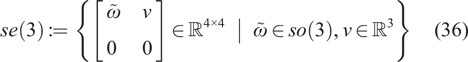
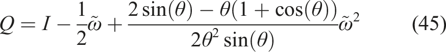
Concerning notation for the relative twists (velocities) of rigid bodies: Consider a curve $H_B^A:\mathbb{R}\to SE\left(3\right),then\hspace{0.17em}twists\hspace{0.17em}\stackrel{\sim }{T}\in se\left(3\right)$ appear as the left- and right-translated change-rates ${\dot{H}}_B^A=d/dt{H}_B^A\left(t\right)$ by

${\stackrel{\sim }{T}}_B^{B,A}=H_A^B{\dot{H}}_B^A,\hspace{1em}{\stackrel{\sim }{T}}_B^{A,A}={\dot{H}}_B^A{H}_A^B$

(39)

Both ${\stackrel{\sim }{T}}_B^{B,A}$ and ${\stackrel{\sim }{T}}_B^{A,A}$ represent the generalized velocity (twist) of frame Ψ _B with respect to Ψ _A , but ${\stackrel{\sim }{T}}_B^{B,A}$ is expressed in Ψ _B while ${\stackrel{\sim }{T}}_B^{A,A}$ is expressed in Ψ _A (Murray et al., 1994, Ch. 2.4).

The adjoint representations of so(3) and se(3) follow from the definition (6) as

${\text{ad}}_{\omega }=\mathrm{\Lambda }\left(\omega \right),{\text{ad}}_T=\left[\begin{array}{ll}\mathrm{\Lambda }\left(\omega \right)& 0\\ \mathrm{\Lambda }\left(v\right)& \mathrm{\Lambda }\left(\omega \right)\end{array}\right]$

(40)

The exponential maps for SO(3) and SE(3) are almost-global diffeomorphisms that relate $\stackrel{\sim }{\omega }\in so\left(3\right)$ to R ∈ SO(3) via (41) and $\stackrel{\sim }{T}\in se\left(3\right)$ to H ∈ SE(3) via (42) (Murray et al., 1994, App. A, Sec. 2.3):

$e^{\stackrel{\sim }{\omega }}={\displaystyle \sum }_{n=0}^{\infty }\frac{1}{n!} {\stackrel{\sim }{\omega }}^n=I+\sin \left(\theta \right) \stackrel{\sim }{\widehat{\omega }}+\left(1-\hspace{0.17em}\cos \left(\theta \right)\right){\stackrel{\sim }{\widehat{\omega }}}^2,$

(41)

$e^{\stackrel{\sim }{T}}={\displaystyle \sum }_{n=0}^{\infty }\frac{1}{n!} {\stackrel{\sim }{T}}^n=\left[\begin{array}{ll}{e}^{\stackrel{\sim }{\omega }}& \frac{1}{{\theta }^2}\left(I-e^{\stackrel{\sim }{\omega }}\right)\stackrel{\sim }{\omega }v+{\omega }^{\top }v\omega \\ 0& 1\end{array}\right]$

(42)

with $\theta ={\Vert \omega \Vert }_2=\sqrt{{\omega }^{\top }\omega }$ and $\stackrel{\sim }{\widehat{\omega }}=\stackrel{\sim }{\omega }/\theta$ .

For θ < π their inverses are presented in equations (43) and (44), respectively: the log map for SO(3) is (Murray et al., 1994, Appendix A, Section 2.3)

$\log \left(R\right)=\{\begin{array}{ll}{\cos }^{-1}\left(\frac{1}{2}\left(\text{Tr}\left(R\right)-1\right)\right)\frac{A}{\Vert A\Vert },& R\ne I,\\ 0_{3\times 3},& R=I,\end{array}$

(43)

with A = 1/2(R − R ^⊤ ) the anti-symmetric part of R, while $\Vert A\Vert :=\sqrt{-1/2\text{Tr}\left(A^2\right)}$ .

Denoting $\stackrel{\sim }{\omega }=\log \left(R\right)$ , the log map for SE(3) is (Murray et al. (1994), Appendix A, Section 2.3)

$\log \left(\left[\begin{array}{ll}R& p\\ 0& 1\end{array}\right]\right)=\left[\begin{array}{ll}\stackrel{\sim }{\omega }& Qp\\ 0& 0\end{array}\right],$

(44)

$Q=I-\frac{1}{2}\stackrel{\sim }{\omega }+\frac{2\hspace{0.17em}\sin \left(\theta \right)-\theta \left(1+\cos \left(\theta \right)\right)}{2{\theta }^2\hspace{0.17em}\sin \left(\theta \right)}{\stackrel{\sim }{\omega }}^2$

(45)

Since lim_θ→0 Q = I, a well-defined Q is given by (45) regardless of R, such that the logarithm on SE(3) (44) has the range of validity of the logarithm on SO(3) (43), bounded only by the rotational part.

4.2 Minimal atlas

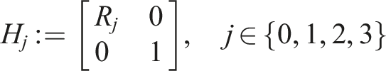
Here we construct minimal exponential atlases for SO(3) and SE(3) as special cases of the exponential atlas (21) – (23) for the respective Lie groups. Both atlases use four charts, which is the theoretical minimum size of an atlas for SO(3) and SE(3) (Grafarend and Kühnel, 2011).

For the atlas on SO(3) the four exponential charts are centered on the elements

$\begin{array}{l}{R}_0=\left[\begin{array}{lll}1& 0& 0\\ 0& 1& 0\\ 0& 0& 1\end{array}\right],R_1=\left[\begin{array}{lll}1& 0& 0\\ 0& -1& 0\\ 0& 0& -1\end{array}\right],\\ R_2=\left[\begin{array}{lll}-1& 0& 0\\ 0& 1& 0\\ 0& 0& -1\end{array}\right],R_3=\left[\begin{array}{lll}-1& 0& 0\\ 0& -1& 0\\ 0& 0& 1\end{array}\right]\end{array}$

The full minimal atlas for SO(3) is then given by

$\begin{array}{llll}{\mathcal{A}}_{\min }^{SO\left(3\right)}& :=& \left\{\left(U_j,x_j\right)|j\in \left\{0,1,2,3\right\}\right\}& ,\end{array}$

(46)

$\begin{array}{llll}{U}_j& :=& \left\{R_j{e}^{\stackrel{\sim }{\omega }}|\omega \in {\mathbb{R}}^3,\left|\omega \right|<\pi \right\}& ,\end{array}$

(47)

$\begin{array}{llll}{x}_j\left(R\right)& :=& {\mathrm{\Lambda }}^{-1}\hspace{0.17em}\log \left(R_j^{\top }R\right)& ,\end{array}$

(48)

$\begin{array}{llll}{x}_j^{-1}\left(q_j\right)& & =R_j{e}^{\mathrm{\Lambda }\left(q_j\right)}& \end{array}$

(49)

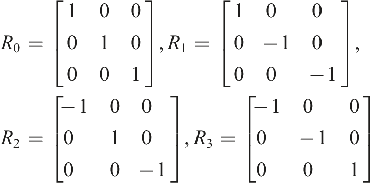
Intuitively speaking, the open set U _j contains all orientations that are reachable from R _j by a rotation through an angle less than π.

A proof that ${\mathcal{A}}_{\min }^{SO\left(3\right)}$ covers SO(3) is shown in Appendix B.3.

For the atlas on SE(3), define the centers of the exponential charts on SE(3) as

$H_j:=\left[\begin{array}{ll}{R}_j& 0\\ 0& 1\end{array}\right],j\in \left\{0,1,2,3\right\}$

The full minimal atlas on SE(3) is then given by

$\begin{array}{llll}{\mathcal{A}}_{\min }^{SE\left(3\right)}& :=& \left\{\left({\mathcal{U}}_j,{\mathcal{X}}_j\right)|\left(U_j,x_j\right)\in {\mathcal{A}}_{\min }^{SO\left(3\right)}\right\}& ,\end{array}$

(50)

$\begin{array}{llll}{\mathcal{U}}_j& :=& \left\{\left[\begin{array}{ll}R& p\\ 0& 1\end{array}\right]|R\in U_j,p\in {\mathbb{R}}^3\right\}& ,\end{array}$

(51)

$\begin{array}{llll}{\mathcal{X}}_j\left(H\right)& :=& {\mathrm{\Lambda }}^{-1}\hspace{0.17em}\log \left(H_j^{-1}H\right)& ,\end{array}$

(52)

$\begin{array}{lll}{\mathcal{X}}_j^{-1}\left(q_j\right)& =H_j{e}^{\mathrm{\Lambda }\left(q_j\right)}& \end{array}$

(53)

4.3 Expressing scalar functions

We briefly highlight how to represent scalar-valued functions $F_{SO\left(3\right)}:SO\left(3\right)\to \mathbb{R}$ and $F_{SE\left(3\right)}:SE\left(3\right)\to \mathbb{R}$ . One approach is to define functions on manifolds by restricting a function defined on an embedding space ${\mathbb{R}}^{n\times n}$ (Falorsi and Forré, 2020). For Lie groups, it is immediately applicable whenever a matrix representation is available.

For example, on SE(3) one restricts a function $F_{{\mathbb{R}}^{4\times 4}}:{\mathbb{R}}^{4\times 4}\to \mathbb{R}$ to arguments from $SE\left(3\right)\subset {\mathbb{R}}^{4\times 4}$ , see Figure 3. The gradient of such functions are computed by an application of equation (31):

${\mathrm{d}}_H{F}_{SE\left(3\right)}=\frac{\partial }{\partial q}{F}_{SE\left(3\right)}{\left(H\left(I+\stackrel{\sim }{q}\right)\right)}_{q=0}$

(54)

Figure 3.

Commutative diagram highlighting how the natural embedding 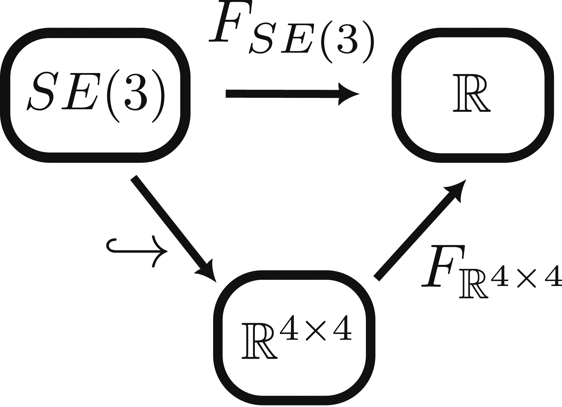$\hookrightarrow :SE\left(3\right)\to {\mathbb{R}}^{4\times 4}$ can be used to restrict a general matrix function to SE(3).

The approach also holds for SO(3), which can be embedded in ${\mathbb{R}}^{3\times 3}$ , instead of ${\mathbb{R}}^{4\times 4}$ .

5. Optimizing a rigid body control

The optimization procedure in Section 2 is applied to potential energy and damping injection based control of a fully actuated rigid body.

The core idea of potential energy shaping and damping injection is to combine advantages of energy-balancing passivity based control (EB-PBC) (Ortega and Mareels, 2000) and of control by interconnection (Ortega et al., 2008), which provide stability guarantees when interfacing with physical systems. Our article presents a class of controllers that generalizes the architecture presented by Rashad et al. (2019). We address common safety concerns about machine learning in control loops by optimizing a class of controllers that guarantees stability and a bounded energy by design.

5.1 Control of a rigid body

The trajectory of a rigid body in Euclidean 3-space is fully described by the curve $H_b^0:\mathbb{R}\to SE\left(3\right)$ that gives the relative position and orientation of a frame Ψ _b attached to the rigid body with respect to an inertial frame Ψ₀ (see Remark 4.1). Following equation (39), the twist of the body with respect to Ψ₀, expressed in the body frame Ψ _b is

$T_b^{b,0}={\mathrm{\Lambda }}^{-1}\left(H_0^b{\dot{H}}_b^0\right)$

(55)

Given the inertia tensor $\mathcal{I}\in {\mathbb{R}}^{6\times 6}$ , $P^b=\mathcal{I}{T}_b^{b,0}\in {\mathbb{R}}^6$ represents the momentum in the body frame. The indices remain fixed in the subsequent treatment, and are suppressed to avoid cluttering (i.e., $H:=H_b^0,T:=T_b^{b,0},P:=P^b$ ).

The dynamics of a rigid body follow from the Hamiltonian equations on matrix Lie groups ((100) and (101) in Appendix A.2) by setting G = SE(3) and letting $\mathcal{H}\left(H,P\right)=1/2P^{\top }{\mathcal{I}}^{-1}P$ . Including an external input wrench $W\in {\mathbb{R}}^6$ , the dynamics read:

$\begin{array}{ll}\dot{H}& =H\mathrm{\Lambda }\left({\mathcal{I}}^{-1}P\right),\end{array}$

(56)

$\begin{array}{ll}\dot{P}& ={\text{ad}}_{{\mathcal{I}}^{-1}P}^{\top }P+W\end{array}$

(57)

In control by potential energy shaping and damping injection, this external wrench is constructed as a sum of a potential gradient term W _V and a damping term W _D :

$W=W_V+W_D$

(58)

In our approach the potential gradient term

$W_V=-{\mathrm{d}}_{H}V$

(59)

is computed by an application of equation (54).

Nonlinear, configuration-dependent viscous damping takes the form

$W_D=-B\left(H,P\right)P$

(60)

with $B\left(H,P\right)\mathcal{I}\in {\mathbb{R}}^{6\times 6}$ a symmetric and positive definite matrix. ⁴

Remark 5.1

In this context, the control architecture of Rashad et al. (2019) corresponds to the popular yet very particular choice of a constant B(H, P) for the damping injection, while their potential V(H) shows a quadratic dependence on translations and a nearly quadratic dependence on rotations. Their controller may be interpreted as a linear PD controller on SE(3), where our work may be seen as a nonlinear PD controller on SE(3).

5.2 Stability

We present here a general proof of stability for the class of controllers.

Theorem 5.1

Stability. Given the system (56), (57) together with the controller (58) given as

$W\left(H,P\right)=-d_{H}V-B\left(H,P\right)P$

(61)

If $\forall H\in SE\left(3\right),P\in {\mathbb{R}}^6:B\left(H,P\right)\mathcal{I}>0$ and $V:SE\left(3\right)\to \mathbb{R}$ is lower-bounded, then lim_t→∞P(t) = 0 and any local minimum of V is locally asymptotically stable.

Proof. With E_Pot = V(H) and ${\mathrm{E}}_{\text{Kin}}=1/2P^{\top }{\mathcal{I}}^{-1}P$ , take the system’s total energy E = E_Pot + E_Kin as the Lyapunov function candidate. Then

$\begin{array}{ll}{\stackrel{.}{\mathrm{E}}}_{\text{Pot}}& ={\left({\mathrm{d}}_{H}V\right)}^{\top }T\end{array}$

(62)

$\begin{array}{l}\begin{array}{ll}{\stackrel{.}{\mathrm{E}}}_{\text{Kin}}& ={\left(\dot{P}\right)}^{\top }{\mathcal{I}}^{-1}P={\left(\dot{P}\right)}^{\top }T\end{array}\\ ={\left({\text{ad}}_T^{\top }P-{\mathrm{d}}_{H}V\right)}^{\top }T-{\left(P\right)}^{\top }BT\\ ={\left(-{\mathrm{d}}_{H}V\right)}^{\top }T-T^{\top }B\mathcal{I}T,\end{array}$

(63)

such that

$\stackrel{.}{\mathrm{E}}={\stackrel{.}{\mathrm{E}}}_{\text{Pot}}+{\stackrel{.}{\mathrm{E}}}_{\text{Kin}}=-T^{\top }B\mathcal{I}T\le 0$

(64)

By LaSalle’s invariance principle, the system converges to the greatest invariant subset where $\dot{E}=0$ . Since B(H, P) > 0, the set with $\dot{E}=0$ is simply the set

$S=\left\{\left(H,P\right)|P=0\right\}$

(65)

By inspection of the dynamics (57) the greatest invariant subset of S is the set with d _H V = 0, corresponding to the maxima and minima of V. Since $\dot{E}\le 0$ , the system cannot converge to maxima of V, leaving the minima of V as limit sets and local minima of V as asymptotically stable equilibria.

5.3 Optimization by the adjoint method on SE(3)

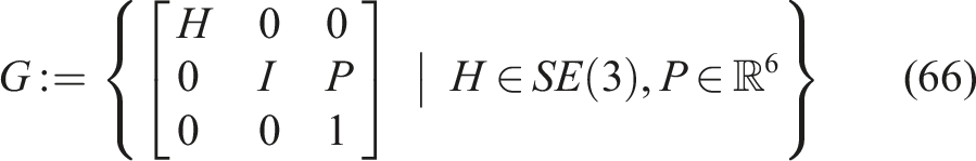
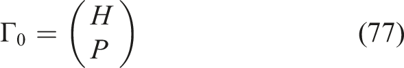
In order to apply the adjoint method on Lie groups (Theorem 2.1), we re-define the dynamics (56) and (57) on the Lie group G = SE(3) × se*(3). To this end, we choose to equip G with the element-wise composition (H₁, P₁) ◦ (H₂, P₂) = (H₁H₂, P₁ + P₂).

As a composition of matrix Lie groups SE(3) and $\left({\mathbb{R}}^6,+\right)$ , $G\subset GL\left(11,\mathbb{R}\right)$ is defined as

$G:=\left\{\left[\begin{array}{lll}H& 0& 0\\ 0& I& P\\ 0& 0& 1\end{array}\right]|H\in SE\left(3\right),P\in {\mathbb{R}}^6\right\}$

(66)

where matrix multiplication indeed corresponds to the element-wise composition in the abstract G. For details on the construction of G, the Lie algebra $\mathfrak{g}$ , the choice of Lie algebra representation $\mathrm{\Lambda }:{\mathbb{R}}^{12}\to \mathfrak{g}$ , adjoint map and exponential map see Appendix B.5.2. The dynamics for Γ(t) ∈ G read

$\dot{\mathrm{\Gamma }}=f_{\theta }\left(\mathrm{\Gamma }\right)=\left[\begin{array}{lll}\dot{H}\left(H,P\right)& 0& 0\\ 0& 0& {\dot{P}}_{\theta }\left(H,P\right)\\ 0& 0& 0\end{array}\right]$

(67)

where

$\begin{array}{ll}\dot{H}\left(H,P\right)& =H\mathrm{\Lambda }\left({\mathcal{I}}^{-1}P\right),\end{array}$

(68)

$\begin{array}{ll}{\dot{P}}_{\theta }\left(H,P\right)& ={\text{ad}}_{{\mathcal{I}}^{-1}P}^{\top }P+W_{\theta }\left(H,P\right)\end{array}$

(69)

Here, the control-wrench $W_{\theta }:SE\left(3\right)\times {\mathbb{R}}^6\to {\mathbb{R}}^6$ is parameterized by $\theta \in {\mathbb{R}}^{n_{\theta }}$ .

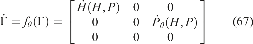
Given a cost $C_{f_{\theta }}^T\left(\mathrm{\Gamma },\theta \right)$ of the type (10) and a distribution $\mathbb{P}$ of initial conditions Γ₀, define an optimization problem in the form of (11):

$\underset{\theta }{\min }{\mathbb{E}}_{{\mathrm{\Gamma }}_0\mathbb{\sim }\mathbb{P}\left({\mathrm{\Gamma }}_0\right)}\left[C\left({\mathrm{\Gamma }}_0,\theta \right)\right]=\underset{\theta }{\min }J\left(\theta \right)$

(70)

As in Section 2.3, approximate $J\left(\theta \right)\approx {\sum }_{i=0}^N{C}_{f_{\theta }}^T\left({\mathrm{\Gamma }}_i,\theta \right)$ and apply Theorem 2.1 to compute the parameter gradient of the $C_{f_{\theta }}^T\left({\mathrm{\Gamma }}_i,\theta \right)$ by equation (15).

The dynamics of λ_Γ follow from equation (17) as

${\stackrel{.}{\lambda }}_{\mathrm{\Gamma }}=-{\mathrm{d}}_{\mathrm{\Gamma }}\left({\lambda }_{\mathrm{\Gamma }}\left({\mathrm{\Lambda }}^{-1}({\stackrel{\sim }{f}}_{\theta }\left(\mathrm{\Gamma }\right)\right)+r\left(\mathrm{\Gamma },\theta \right)\right)+{\text{ad}}_{{\stackrel{\sim }{f}}_{\theta }}^{\top }{\lambda }_{\mathrm{\Gamma }},$

(71)

${\lambda }_{\mathrm{\Gamma }}\left(T\right)={\mathrm{d}}_{\mathrm{\Gamma }}F$

(72)

where ${\mathrm{\Lambda }}^{-1}\left({\stackrel{\sim }{f}}_{\theta }\right)$ is

${\mathrm{\Lambda }}^{-1}\left({\stackrel{\sim }{f}}_{\theta }\right):={\mathrm{\Lambda }}^{-1}\left({\mathrm{\Gamma }}^{-1}{f}_{\theta }\left(\mathrm{\Gamma }\right)\right)=\left(\begin{array}{l}{\mathcal{I}}^{-1}P\\ {\dot{P}}_{\theta }\left(H,P\right)\end{array}\right)$

(73)

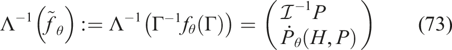
The gradient ${\mathrm{d}}_{\mathrm{\Gamma }}:C^1\left(G,\mathbb{R}\right)\to {\mathbb{R}}^{12}$ is given by equation (31). We split it into components ${\mathrm{d}}_H:C^1\left(SE\left(3\right),\mathbb{R}\right)\to {\mathbb{R}}^6$ and ${\mathrm{d}}_P:C^1\left(\text{Vec}\left(6,\mathbb{R}\right),\mathbb{R}\right)\to {\mathbb{R}}^6$ defined on the Lie groups SE(3) and $\left({\mathbb{R}}^6,+\right)$ , respectively.

Further, split λ_Γ = (λ _H , λ _P ) into components ${\lambda }_H,{\lambda }_P\in {\mathbb{R}}^6$ , and write out the control-wrench W _θ (H, P) = −d _H V _θ − B _θ (H, P)P. Then the equation for ${\stackrel{.}{\lambda }}_{\mathrm{\Gamma }}$ can be resolved to

${\stackrel{.}{\lambda }}_{\mathrm{\Gamma }}=$

(74)

$\left(\begin{array}{l}{\mathrm{d}}_H\left({\lambda }_P^{\top }\left({\mathrm{d}}_H{V}_{\theta }+B_{\theta }\left(H,P\right)P\right)-r\left(\mathrm{\Gamma },\theta \right)\right)-{\text{ad}}_{{\mathcal{I}}^{-1}P}^{\top }{\lambda }_H\\ {\mathrm{d}}_P\left({\lambda }_P^{\top }\left(B_{\theta }\left(H,P\right)P-{\text{ad}}_{{\mathcal{I}}^{-1}P}^{\top }P\right)-r\left(\mathrm{\Gamma },\theta \right)\right)-{\mathcal{I}}^{-1}{\lambda }_H\end{array}\right),$

${\mathrm{\Lambda }}_H\left(T\right)={\mathrm{d}}_{H}F,{\mathrm{\Lambda }}_P\left(T\right)={\mathrm{d}}_{P}F.$

Remark 5.2

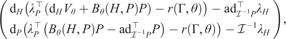
Note that the second derivative term $d_H\left({\lambda }_P^{\top }\left(d_H{V}_{\theta }\right)\right)$ in the dynamics (74) is well-defined, since ${\lambda }_P^{\top }\left(d_H{V}_{\theta }\right)\in C^1\left(SE\left(3\right),\mathbb{R}\right)$ .

Remark 5.3

Rather than constructing the direct product group SE(3) × se*(3), the semi-direct product group SE(3) ⋉ se*(3) could have been defined using the Coadjoint representation $AdH*:{se}^{*}\left(3\right)\to se*\left(3\right),leading\hspace{0.17em}to\hspace{0.17em}the\hspace{0.17em}group\hspace{0.17em}operation\hspace{0.17em}\left(H_1,P_1\right)•\left(H_2,P_2\right)=\left(H_1{H}_2,P_1+A{d}_{H_1}^{*}{P}_2\right)$ . Since an alternative choice of group action does not affect the optimum of the optimization, use of the semi-direct product group was not further investigated.

6. Simulations

We numerically solve the optimization problem (11) for the dynamics (67). We investigate various choices of final and running costs, distributions $\mathbb{P}$ and parameterizations of V _θ , B _θ .

6.1 Quadratic vs. general potential shaping

A controller with quadratic potential and linear damping injection (Section 6.1.2) is compared to a controller with NN-parameterized potential and damping injection (Section 6.1.3).

6.1.1 Choice of cost C and distribution $\mathbb{P}$

We determine a final cost F and a running cost r to stabilize a static target state with H = H _F , p = 0 over a horizon of T = 3 seconds. The key properties of F and r are that both are differentiable and have their minimum in the target pose. Denote components of H and P

$H=\left[\begin{array}{ll}R& p\\ 0& 1\end{array}\right],P=\left(\begin{array}{l}{P}_{\omega }\\ P_v\end{array}\right)$

where $R\in {\mathbb{R}}^{3\times 3}$ , and $p,P_{\omega },P_v\in {\mathbb{R}}^3$ . With weights $w_1,\cdots ,w_9\in {\mathbb{R}}_{+}$ , we choose F and r as

$\begin{array}{ll}F\left(\mathrm{\Gamma }\right)& =-w_1\text{Tr}\left(H_F^{-1}H\right)+w_2\Vert p{\Vert }_2^2\end{array}$

(75)

$+w_3\Vert P_{\omega }{\Vert }^2+w_4\Vert P_v{\Vert }_2^2,$

$\begin{array}{ll}r\left(\mathrm{\Gamma }\right)& =-w_5\text{Tr}\left(H_F^{-1}H\right)+w_6\Vert p{\Vert }_2^2\end{array}$

(76)

$+w_7{{\Vert P_{\omega }\Vert }^2+w_8\Vert P_v{\Vert }_2^2+w_9\Vert W_{\theta }\left(H,P\right)\Vert }^2$

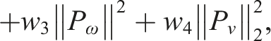
Given scalars $\alpha ,d,{\theta }_p,d_p\mathbb{\in }\mathbb{R}$ and vectors $\omega ,v,{\omega }_p,v_p\in {\mathbb{R}}^3$ , and an average initial pose H _I = H _F , an initial condition Γ₀ is constructed as

${\mathrm{\Gamma }}_0=\left(\begin{array}{l}H\\ P\end{array}\right)$

(77)

$q=\left(\begin{array}{l}\alpha \omega /{\Vert \omega \Vert }_2\\ dv/\Vert v{|}_2\end{array}\right),$

(78)

$H=H_I\hspace{0.17em}\exp \left(\stackrel{\sim }{q}\right),$

(79)

$P=\left(\begin{array}{l}{\alpha }_p{\omega }_p/{\Vert {\omega }_p\Vert }_2\\ d_p{v}_p/\Vert v_p{|}_2\end{array}\right)$

(80)

The distribution $\mathbb{P}$ of Γ₀ is implemented by sampling

$\alpha \sim \text{Uniform}\left[0,\pi \right],d\sim \text{Uniform}\left[0,1\right],$

(81)

${\alpha }_p\sim \text{Uniform}\left[0,0.03\right],d_p\sim \text{Uniform}\left[0,1\right]$

(82)

and sampling $\omega ,v,{\omega }_p,v_p\in {\mathbb{R}}^3$ from a normal distribution $\mathcal{N}\left(\mu ,{\sigma }^2\right)$ with standard deviation μ = (0,0,0) ^T and variance σ² = I_3×3.

6.1.2 Quadratic potential and linear damping injection

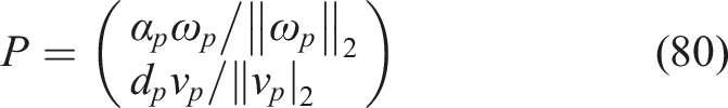
The quadratic controller coincides with the controller presented by Rashad et al. (2019), in a setting of motion control. As such the quadratic potential $V_{Q,\theta }:SE\left(3\right)\to \mathbb{R}$ is given by

$\begin{array}{ll}{V}_{Q,\theta }\left(\left[\begin{array}{ll}R& p\\ 0& 1\end{array}\right]\right)=& \frac{1}{4}{p}^{\top }{K}_{\theta }p+\frac{1}{4}{p}^{\top }R{K}_{\theta }{R}^{\top }p\end{array}$

(83)

$-\text{Tr}\left(G_{\theta }\left(R-I_3\right)\right),$

and the constant damping injection is characterized by

$B_{Q,\theta }\left(H,P\right)=B_{Q,\theta }\in {\mathbb{R}}^{6\times 6}$

(84)

Here the translational stiffness matrix $K_{\theta }\in {\mathbb{R}}^{3\times 3}$ , the rotational co-stiffness matrix $G_{\theta }\in {\mathbb{R}}^{3\times 3}$ and the damping injection matrix B_Q,θ are chosen as

$\begin{array}{ll}{K}_{\theta }& =\left[\begin{array}{lll}\exp \left({\theta }_1\right)& 0& 0\\ 0& \exp \left({\theta }_2\right)& 0\\ 0& 0& \exp \left({\theta }_3\right)\end{array}\right]\end{array}$

(85)

$\begin{array}{ll}{G}_{\theta }& =\left[\begin{array}{lll}\exp \left({\theta }_4\right)& 0& 0\\ 0& \exp \left({\theta }_5\right)& 0\\ 0& 0& \exp \left({\theta }_6\right)\end{array}\right]\end{array}$

(86)

$\begin{array}{ll}{B}_{Q,\theta }& =\left[\begin{array}{llllll}\exp \left({\theta }_7\right)& 0& 0& 0& 0& 0\\ 0& \exp \left({\theta }_8\right)& 0& 0& 0& 0\\ 0& 0& \exp \left({\theta }_9\right)& 0& 0& 0\\ 0& 0& 0& \exp \left({\theta }_{10}\right)& 0& 0\\ 0& 0& 0& 0& \exp \left({\theta }_{11}\right)& 0\\ 0& 0& 0& 0& 0& \exp \left({\theta }_{12}\right)\end{array}\right]\end{array}$

(87)

where the diagonal elements exp(θ _i ) ensure that the matrices are positive definite. Note that the conditions of Theorem 5.1 are guaranteed: V _Q is lower-bounded, and symmetry of $B_{Q,\theta }\mathcal{I}$ is guaranteed since B_Q,θ is diagonal and positive definite.

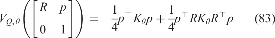
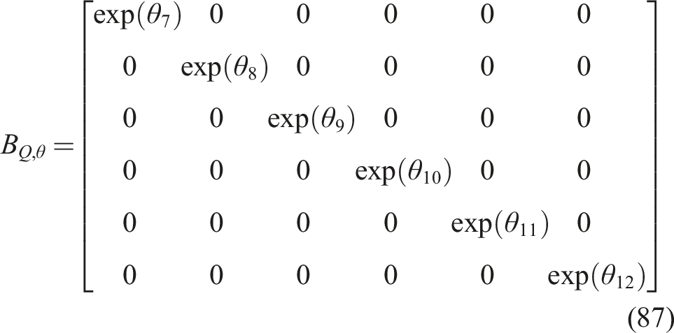
The control-law is then of the form

$W_{Q,\theta }\left(H,P\right)=-{\mathrm{d}}_H{V}_{Q,\theta }-B_{Q,\theta }P$

(88)

The parameters are optimized over 1200 training epochs, using the ADAM optimizer with decay γ = 0.999, a learning rate of η = 0.001 for the initial 1000 epochs and restarting training at a learning rate of η = 0.01 for the final 200 epochs. Additional parameters of the training are summarized in Appendix C.1, Table 1. The training progress is summarized in Figure 4, where Figure 4(a) shows a monotonous decrease of the cost function over the training epochs, while Figures 4(b) and 4(c) indicate a steady improvement of the final system states with respect to the target pose. The resulting controller’s performance is shown in Figure 5. Here Figures 5(a) and 5(b) show that the controlled rigid bodies approach the target configuration. Figure 5(c) shows that the controller uses the potential V_Q,θ to guide the rigid bodies towards the target pose, and that kinetic energy is quickly dissipated.

Table 1.

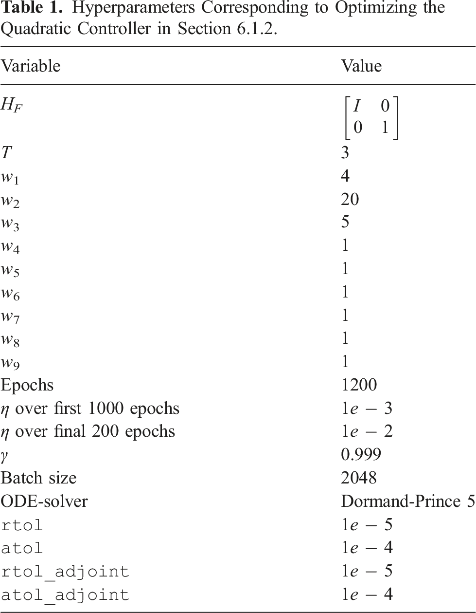
Hyperparameters Corresponding to Optimizing the Quadratic Controller in Section 6.1.2.

Variable	Value
H F	$\left[\begin{array}{ll}I& 0\\ 0& 1\end{array}\right]$
T	3
w 1	4
w 2	20
w 3	5
w 4	1
w 5	1
w 6	1
w 7	1
w 8	1
w 9	1
Epochs	1200
η over first 1000 epochs	1e − 3
η over final 200 epochs	1e − 2
γ	0.999
Batch size	2048
ODE-solver	Dormand-Prince 5
rtol	1e − 5
atol	1e − 4
rtol_adjoint	1e − 5
atol_adjoint	1e − 4

Figure 4.

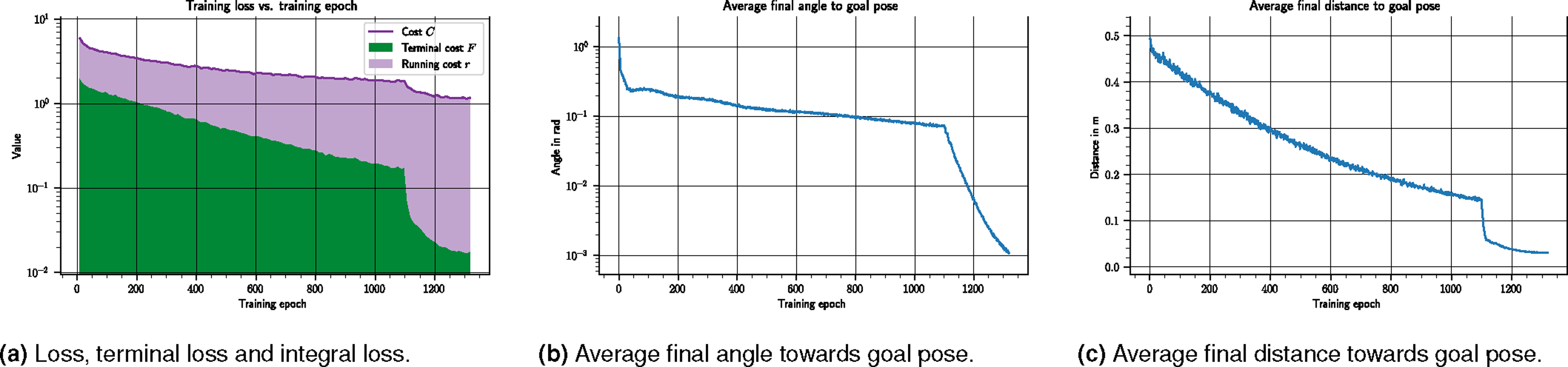
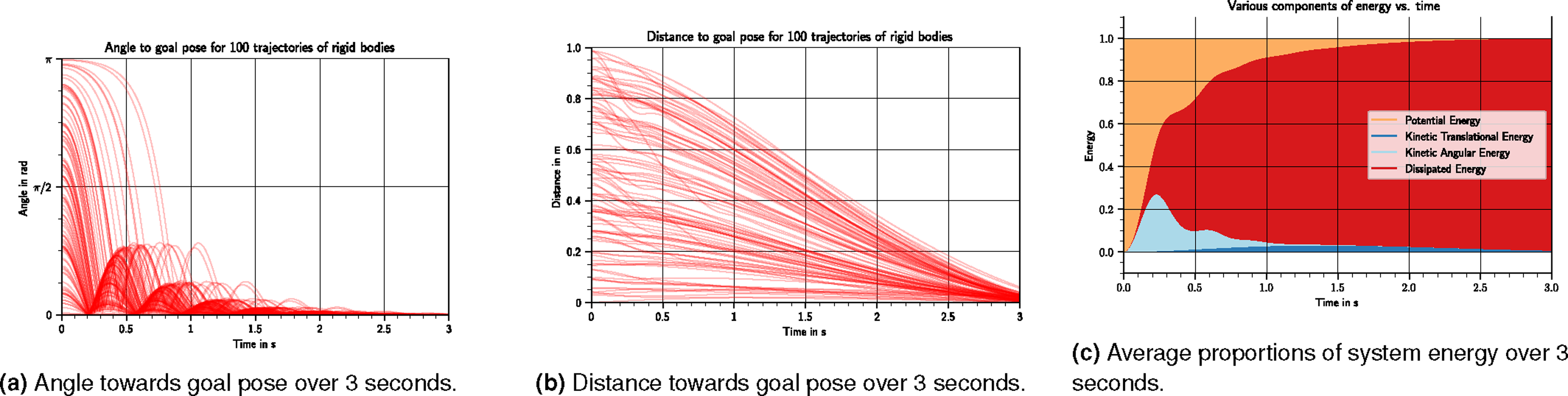
Visualization of the training progress of the quadratic controller characterized by V_Q,θ and B_Q,θ. All figures show data averaged over 2048 sample trajectories at the given epoch, with initial conditions sampled from $\mathbb{P}\left({\mathrm{\Gamma }}_0\right)$ .

Figure 5.

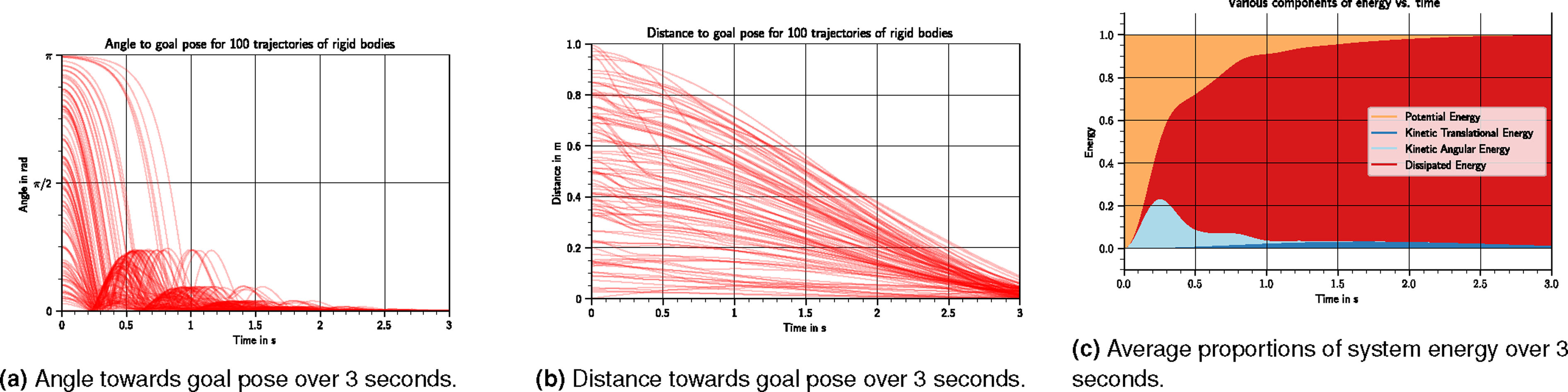
Visualization of the performance of the quadratic controller characterized by V_Q,θ and B_Q,θ, over 100 trajectories of rigid bodies with initial conditions sampled from $\mathbb{P}\left({\mathrm{\Gamma }}_0\right)$ .

6.1.3 Nonlinear potential and damping injection

Here we showcase the optimization of a nonlinear potential $V_{N,\theta }:SE\left(3\right)\to \mathbb{R}$ and a nonlinear damping injections $B_{N,\theta }\left(H,P\right)\in {\mathbb{R}}^{6\times 6}$ . Both functions are parameterized by neural nets with one hidden layer of 64 neurons, using softplus and tanh activation functions. V_N,θ has 12 inputs (the components of R and p, this is a projection of H) and 1 output, while B_N,θ has 18 inputs (components of R, p and P) and 6 outputs, which are then put through an element-wise exponential function and turned into a diagonal 6 by 6 matrix to guarantee positive-definiteness of $B_{N,\theta }\left(H,P\right)\mathcal{I}$ .

The control-law is of the form

$W_{N,\theta }\left(H,P\right)=-{\mathrm{d}}_H{V}_{N,\theta }-B_{N,\theta }\left(H,P\right)P$

(89)

The parameters are optimized over 1000 training epochs, using the ADAM optimizer with decay γ = 0.999, and a learning rate of η = 0.001. Additional parameters of the training are summarized in Appendix C.1, Table 2.

Table 2.

Hyperparameters Corresponding to Optimizing the nonlinear Controller in Section 6.1.3.

Variable	Value
H F	$\left[\begin{array}{ll}I& 0\\ 0& 1\end{array}\right]$
T	3
w 1	4
w 2	10
w 3	5
w 4	1
w 5	1
w 6	1
w 7	1
w 8	1
w 9	1
Epochs	1200
η over first 1000 epochs	1e − 3
η over final 200 epochs	1e − 3
γ	0.999
Batch size	2048
ODE-solver	Dormand-prince 5
rtol	1e − 5
atol	1e − 4
rtol_adjoint	1e − 5
atol_adjoint	1e − 4

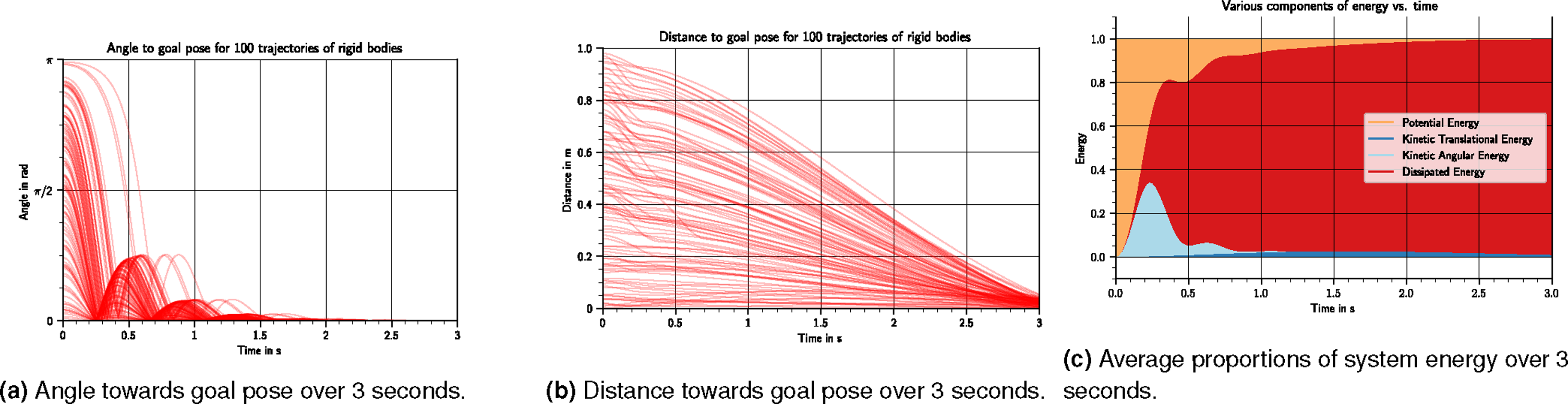
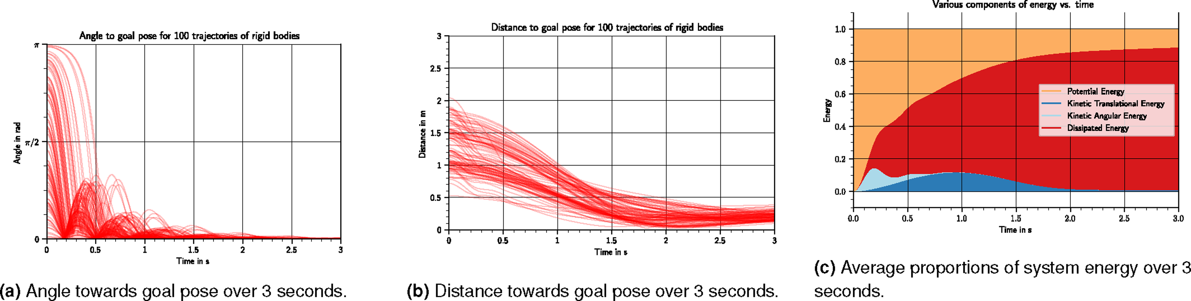
The training progress is summarized in Figure 6. It can be seen that the final loss of the nonlinear controller in Figure 6(a) is equivalent to that of the quadratic controller Figure 4(a). In particular, the performance of a quadratic and a nonlinear controller for this scenario are close: the final angle and distance in Figures 6(b) and 6(c) are comparable to those of Figures 4(b) and 4(c), respectively. The resulting controller’s performance is shown in Figure 7. Here the qualitative behavior shown in Figures 7(a), 7(b) and 7(c) resembles that of the quadratic case in Figures 5(a), 5(b), and 5(c), respectively.

Figure 6.

Visualization of the training progress of the nonlinear controller characterized by V_N,θ and B_N,θ. All figures show data averaged over 2048 sample trajectories at the given epoch, with initial conditions sampled from $\mathbb{P}$ .

Figure 7.

Visualization of the performance of the nonlinear controller characterized by V_N,θ and B_N,θ, over 100 trajectories of rigid bodies with initial conditions sampled from 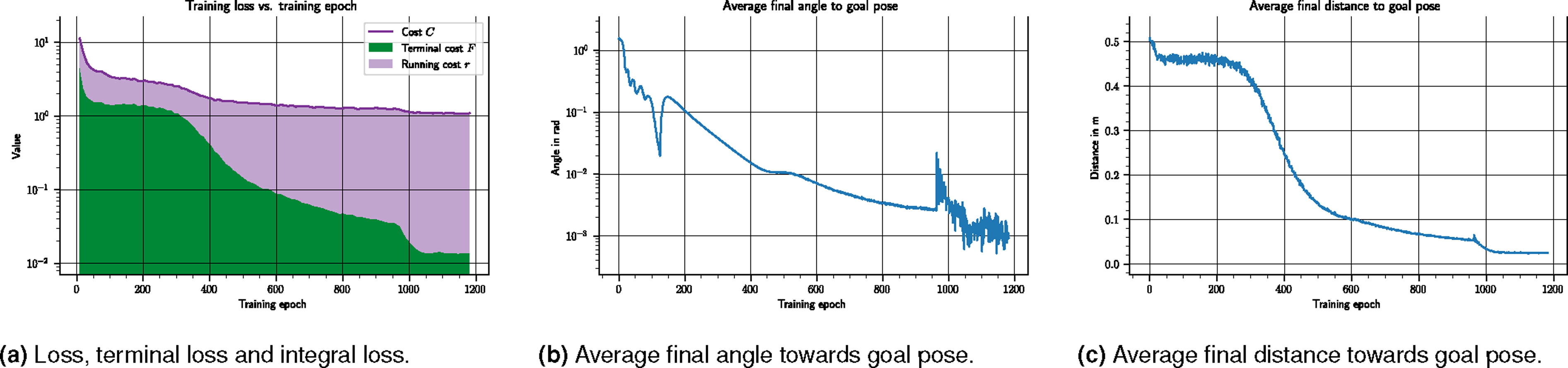$\mathbb{P}\left({\mathrm{\Gamma }}_0\right)$ .

6.2 General potential shaping with gravity

We optimize an NN-parameterized potential and damping injection in a system with gravity in Section 6.2.2, and show the effect of an adapted target configuration in Section 6.2.3.

6.2.1 Adapted running cost r

In the presence of a gravitational potential $V_g:SE\left(3\right)\to \mathbb{R}$ the momentum dynamics of a controlled rigid body (69) pick up an additional term −d _H V _g :

${\dot{P}}_{\theta }\left(H,P\right)={\text{ad}}_{{\mathcal{I}}^{-1}P}^{\top }P+W_{\theta }\left(H,P\right)-{\mathrm{d}}_H{V}_g$

(90)

The gravitational potential is unbounded: it can therefore not be globally compensated for by a bounded potential V_N,θ. To circumvent this issue, we separately implement gravity compensation W _g (H) = d _H V _g by choosing the total control-wrench as

$W_{\theta }\left(H,P\right)=W_g\left(H\right)+W_{N,\theta }\left(H,P\right)$

(91)

such that the momentum dynamics again read

${\dot{P}}_{\theta }\left(H,P\right)={\text{ad}}_{{\mathcal{I}}^{-1}P}^{\top }P+W_{N,\theta }\left(H,P\right)$

(92)

To take gravity into account in the optimization, the only required adaptation is to use the adapted W _θ (H, P) in the running cost (76).

Minimizing the term ‖W _θ (H, P)‖ indirectly minimizes the required gravity compensation by reducing the total wrench exerted on the plant. Indeed, when ‖W _θ ‖ = 0 the dynamics are

${\dot{P}}_{\theta }\left(H,P\right)={\text{ad}}_{{\mathcal{I}}^{-1}P}^{\top }P-{\mathrm{d}}_H{V}_g$

(93)

Thus, for ‖W _θ ‖ = 0 the learned control-action W_N,θ(H, P) cancels the gravity compensation, such that the external gravitational potential is utilized to exert a force on the rigid body.

6.2.2 Nonlinear potential and damping injection

Here, we apply the ADAM optimizer with learning rate η = 0.001 and decay γ = 0.999 to optimize the nonlinear potential V_N,θ and damping B_N,θ for an adapted running cost. Additional parameters of the training are summarized in Appendix C.1, Table 3. The training progress is summarized in Figure 8, and the resulting controller’s performance is shown in Figure 9. Notably, the results do not differ strongly from Figures 6 and 5.

Table 3.

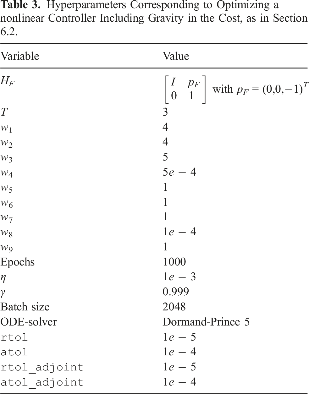
Hyperparameters Corresponding to Optimizing a nonlinear Controller Including Gravity in the Cost, as in Section 6.2.

Variable	Value
H F	$\left[\begin{array}{ll}I& p_F\\ 0& 1\end{array}\right]$ with p F = (0,0,−1) T
T	3
w 1	4
w 2	4
w 3	5
w 4	5e − 4
w 5	1
w 6	1
w 7	1
w 8	1e − 4
w 9	1
Epochs	1000
η	1e − 3
γ	0.999
Batch size	2048
ODE-solver	Dormand-Prince 5
rtol	1e − 5
atol	1e − 4
rtol_adjoint	1e − 5
atol_adjoint	1e − 4

Figure 8.

Visualization of the training progress of the nonlinear controller characterized by V_N,θ and B_N,θ, in the presence of gravity. All figures show data averaged over 2048 sample trajectories at the given epoch, with initial conditions sampled from $\mathbb{P}\left({\mathrm{\Gamma }}_0\right)$ .

Figure 9.

Visualization of the performance of the nonlinear controller characterized by V_N,θ and B_N,θ, in the presence of gravity. The results show 100 trajectories of rigid bodies with initial conditions sampled from $\mathbb{P}\left({\mathrm{\Gamma }}_0\right)$ .

6.2.3 Asymmetric initial distribution

To better highlight the influence of the adapted running cost, and how the optimization in the presence of gravity differs from an optimization in the absence of gravity, an initial distribution asymmetric about the goal pose H _F (77) is introduced by choosing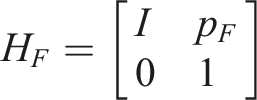

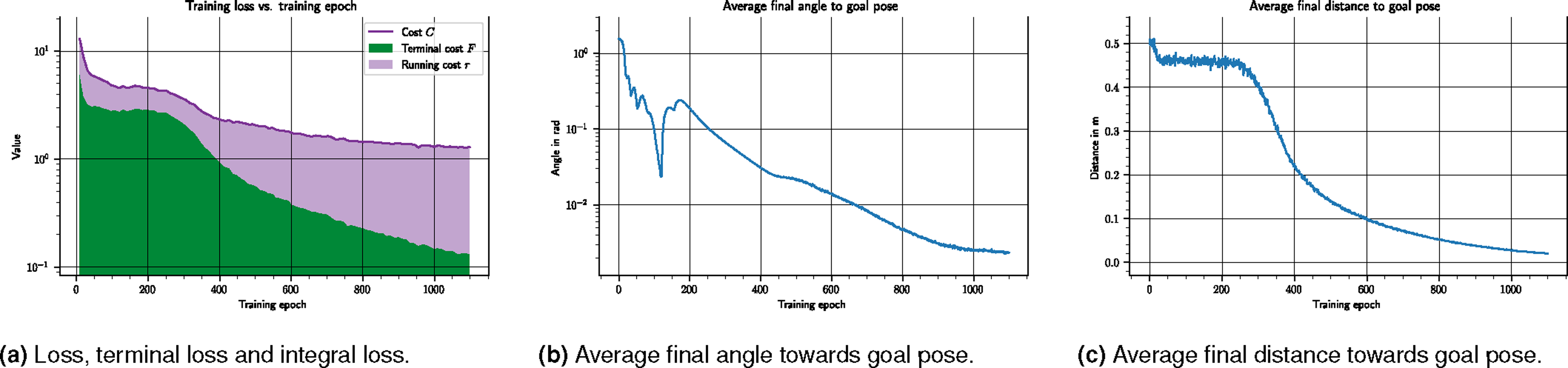
$H_F=\left[\begin{array}{ll}I& p_F\\ 0& 1\end{array}\right]$

with p _F = (0,0,−1) ^T .

The parameters of this training coincide with those of the symmetric scenario, and are likewise summarized in Appendix C.1, Table 3. The training progress is summarized in Figure 10, and the resulting controller’s performance is shown in Figure 11.

Figure 10.

Visualization of the training progress of the nonlinear controller characterized by V_N,θ and B_N,θ, in the presence of gravity and with an initial distribution whose mean is above the target position. All figures show data averaged over 2048 sample trajectories at the given epoch, with initial conditions sampled from $\mathbb{P}\left({\mathrm{\Gamma }}_0\right)$ .

Figure 11.

Visualization of the performance of the nonlinear controller characterized by V_N,θ and B_N,θ, in the presence of gravity and with an initial distribution whose mean is above the target position. The results show 100 trajectories of rigid bodies with initial conditions sampled from 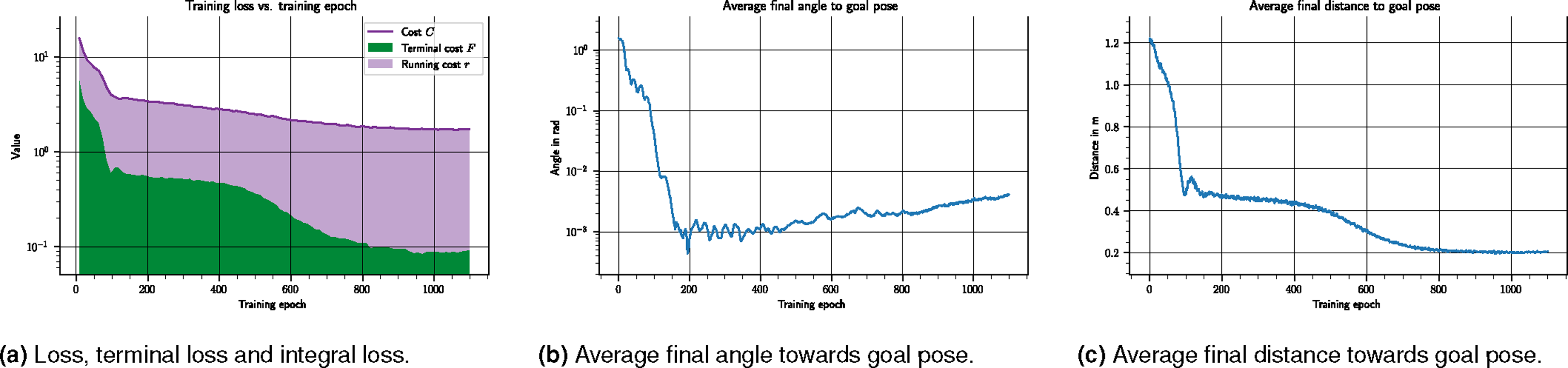$\mathbb{P}\left({\mathrm{\Gamma }}_0\right)$ .

7. Discussion

7.1 Neural ODEs on Lie groups

The proposed formulation of neural ODEs on Lie groups immediately applies to arbitrary matrix Lie groups, where parameterized maps can be learned with a global validity. The optimization of Neural ODEs on Lie groups by the gradient descent via the generalized adjoint method is a scalable approach. The key aspects that contribute to this scalability are: First, the generalized adjoint method on Lie groups preserves the memory efficiency of the generalized adjoint method used for neural ODEs on ${\mathbb{R}}^k$ . Second, the formulation of the adjoint dynamics at the algebra level achieves a dimensionality-reduction with respect to extrinsic formulations of Duong and Atanasov (2021b); Falorsi and Forré (2020). Finally, this formulation at the algebra level also alleviates the need for chart switches of the adjoint state, and it allows for the use of the compact expression (31) of the gradient, bypassing the need for gradient computations in local charts.

The work can be generalized further: Theorem 2.1 assumes the cost to be of the form (10), while the derivation in Appendix A.4 in principle allows for a more general choice of cost that may be of interest in, for example, learning of periodic trajectories (Wotte et al., 2023). The accompanying code is currently written specifically for the Lie group $SE\left(3\right)\times {\mathbb{R}}^6$ , and future work will produce code that is applicable to other matrix Lie groups as well.

7.2 Optimal potential shaping

The optimization of an NN-parameterized potential and damping injection was successful and the large number of parameters used in the optimization confirms that it scales to the large parameter scenario. The optimization was also successful when including gravity in a nonlinear running cost. Stability was guaranteed by design, by implementing the requirements of Theorem 5.1 on the level of architecture and activation functions. As a further advantage the resulting controller is global on SE(3), as opposed to only being applicable in a limited chart region.

Regarding limitations of the approach, the numerical stability of the adjoint method on SE(3) was observed to strongly depend on the smoothness of the running cost, which suggests added value in considering different Lie group integrators that accommodate this lack of smoothness. Lastly, while the structure of the presented controller is highly interpretable and the various components of the energy are readily visualized, the space of possible initial conditions and trajectories remains large, and the high-dimensional state-space obscures low-level properties and a deep understanding of the eventual controller, beyond safety guarantees and numerical verification of stability.

Alternative choices for the final and running costs, as well as the weights in these costs are worth investigating. The design space of possible controllers is also large and other control architectures may be advantageous. In future work the controller will be applied to a real drone, and other cost-functions and control structures will be investigated.

8. Conclusion

Lie groups are ubiquitous in engineering, and so are dynamic systems on Lie groups. We proposed a method for dynamics optimization that works on arbitrary, finite-dimensional Lie groups and for a large class of cost-functions. The resulting method is highly scalable, and more compact than alternative manifold formulations. The key steps in the formulation related to using canonical Lie group structure to create a compact gradient descent algorithm: we phrased the generalized adjoint method at the Lie algebra level, we utilize a compact expression for the gradient as an element of the dual to the Lie algebra, and we use a generic Lie group integrator for dynamics integration. The method was successfully applied to optimize a controller for a rigid body that is globally valid on the Lie group SE(3). A key aspect of choosing the class of controllers was stability by design, which guided the architecture of the neural nets that parameterize the potential energy shaping and damping injection controller.