Non-linearity Measure for POMDP-based Motion Planning

Abstract

Motion planning under uncertainty is essential for reliable robot operation. Despite substantial advances over the past decade, the problem remains difficult for systems with complex dynamics. Most state-of-the-art methods perform search that relies on a large number of forward simulations. For systems with complex dynamics, this generally requires costly numerical integrations, which significantly slows down the planning process. Linearization-based methods have been proposed that can alleviate the above problem. However, it is not clear how linearization affects the quality of the generated motion strategy, and when such simplifications are admissible. To answer these questions, we propose a non-linearity measure, called Statistical-distance-based Non-linearity Measure (SNM), that can identify where linearization is beneficial and where it should be avoided. We show that when the problem is framed as the Partially Observable Markov Decision Process, the value difference between the optimal strategy for the original model and the linearized model can be upper-bounded by a function linear in SNM. Comparisons with an existing measure on various scenarios indicate that SNM is more suitable in estimating the effectiveness of linearization-based solvers. To test the applicability of SNM in motion planning, we propose a simple online planner that uses SNM as a heuristic to switch between a general and a linearization-based solver. Results on a car-like robot with second order dynamics and 4-DOFs and 7-DOFs torque-controlled manipulators indicate that SNM can appropriately decide if and when a linearization-based solver should be used.

1. Introduction

An autonomous robot must be able to compute reliable motion strategies, despite various errors in actuation and prediction of its effect on the robot and its environment, and despite various errors in sensors and sensing. Computing such robust strategies is computationally hard even for a 3-DOFs point robot (Canny and Reif, 1987; Natarajan, 1988). Conceptually, this problem can be solved in a systematic and principled manner when framed as the Partially Observable Markov Decision Process (POMDP) (Kaelbling et al., 1998). A POMDP represents the aforementioned errors as probability distribution functions and estimates the state of the system as probability distribution functions called beliefs. It then computes the best motion strategy with respect to beliefs rather than single states, thereby accounting for the fact that the actual state is never known due to the above errors. Although the concept of POMDPs was proposed in the ‘60s (Sondik, 1971), only recently that POMDPs started to become practical for robotics problems (e.g., (Hoerger et al., 2019; Horowitz and Burdick, 2013; Temizer et al., 2009)). This advancement is achieved by trading optimality with approximate optimality for speed and memory. But even then, in general, computing close to optimal POMDP solutions for systems with complex dynamics remains difficult.

Several general POMDP solvers—solvers that do not restrict the type of dynamics and sensing model of the system, nor the type of distributions used to represent uncertainty—can now compute good motion strategies online with a 1-10 Hz update rate for a number of robotic problems (Kurniawati and Yadav, 2016; Seiler et al., 2015; Silver and Veness, 2010; Ye et al., 2017). However, their speed degrades when the robot has complex non-linear dynamics. To compute a good strategy, today’s POMDP solvers forward simulate the effect of many sequences of actions from different beliefs are simulated. For problems whose dynamics have no closed-form solutions, a simulation run generally invokes many numerical integrations, and complex dynamics tend to increase the cost of each numerical integration, which in turn significantly increases the total planning cost of these methods. Of course, this cost will increase even more for problems that require more or longer simulation runs, such as in problems with long planning horizons.

Many linearized-based POMDP solvers have been proposed (Sun et al., 2015; Agha-mohammadi et al., 2013; van Den Berg et al., 2011,0; Prentice and Roy, 2010). They rely on many forward simulations from different beliefs too, but use a linearized model of the dynamics and sensing for simulation. Together with linearization, many of these methods assume that beliefs are Gaussian distributions. This assumption improves the speed of simulation further, because the subsequent belief after an action is performed, and an observation is perceived can be computed in closed-form. In contrast, the aforementioned general solvers typically represent beliefs as sets of particles and estimate subsequent beliefs using particle filters. Particle filters are particularly expensive when particle trajectories have to be simulated and each simulation run is costly, as is the case for motion planning of systems with complex dynamics. As a result, the linearization-based planners require less time to estimate the effect of performing a sequence of actions from a belief, and therefore can potentially find a good strategy faster than the general method. However, it is known that linearization in control and estimation performs well only when the system’s non-linearity is “weak” (Li, 2012). The question is, what constitute “weak” non-linearity in motion planning under uncertainty? Where will it be useful, and where will it be damaging to use linearization (and Gaussian) simplifications?

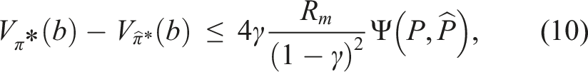
This paper extends our previous work in Hoerger et al. (2020) towards answering the aforementioned questions. Our main contribution is a measure of non-linearity for stochastic systems, called Statistical-distance-based Non-linearity Measure (SNM), to identify the suitability of linearization in a given motion planning under uncertainty problem. SNM is based on the total variation distance between the original dynamics and sensing models, and their corresponding linearized models. It is general enough to be applied to any type of motion and sensing errors, and any linearization technique, regardless of the type of approximation of the true beliefs (e.g., with and without Gaussian simplification). We show that the difference between the value of the optimal strategy generated if we plan using the original model and if we plan using the linearized model, can be upper-bounded by a function linear in SNM. Furthermore, our experimental results indicate that compared to recent state-of-the-art methods of non-linearity measures for stochastic systems, SNM is more sensitive to the effect that obstacles have on the effectiveness of linearization, which is critical for motion planning.

To further test the applicability of SNM in motion planning, we develop a simple online planner that uses a local estimate of SNM to automatically switch between a general planner (Kurniawati and Yadav, 2016) that uses the original POMDP model and a linearization-based planner, adapted from Sun et al. (2015), that uses the linearized model. Experimental results on simulated motion planning under uncertainty problems, including a car-like robot with acceleration control, 4-DOFs and 6-DOFs manipulators with torque control, and a 7-DOFs manipulator in a human-collaboration task indicate that this simple planner can appropriately decide if and when linearization should be used, and therefore computes better strategies faster than each of the component planner.

2. Background and related work

We provide a brief overview of the class of motion planning under uncertainty problems considered in this paper and their POMDP formulation in Section 2.1, followed by a discussion on related measures of non-linearity in Section 2.2.

2.1. Motion planning problems under uncertainty

In this paper, we consider motion planning problems, in which a robot must move from a given initial state to a state in the goal region while avoiding obstacles. The robot operates inside deterministic, bounded, and perfectly known 2D or 3D environments populated by static obstacles.

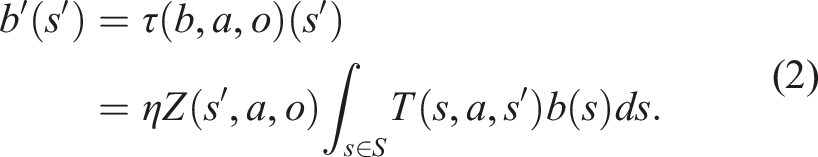
The robot’s transition and observation models are uncertain and defined as follows. Let $S\subset {\mathbb{R}}^n$ be the bounded n-dimensional state space, $A\subset {\mathbb{R}}^d$ the bounded d-dimensional control space and $O\subset {\mathbb{R}}^l$ the bounded l-dimensional observation space of the robot. The state of the robot evolves according to a discrete-time non-linear function, which we model in the general form s_t+1 = f(s _t , a _t , v _t ) where s _t ∈ S is the state of the robot at time t, a _t ∈ A is the control input at time t, and $v_t\in {\mathbb{R}}^d$ is a random transition error. At each time step t, the robot perceives imperfect information regarding its current state according to a non-linear stochastic function of the form o _t = h(s _t , w _t ), where o _t ∈ O is the observation at time t and $w_t\in {\mathbb{R}}^d$ is a random observation error.

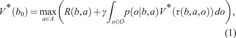
This class of motion planning problems under uncertainty can naturally be formulated as a Partially Observable Markov Decision Process (POMDP). Formally, a POMDP is a tuple ⟨S, A, O, T, Z, R, b₀, γ⟩, where S, A, and O are the state, action, and observation spaces of the robot. T is a conditional probability function T(s, a, s′) = p(s′ | s, a) (where s, s′ ∈ S and a ∈ A) that models the uncertainty in the effect of performing actions, while Z(s′, a, o) = p(o | s′, a) (where o ∈ O) is a conditional probability function that models the uncertainty in perceiving observations. R(s, a) is a reward function, which encodes the planning objective. b₀ is the initial belief, capturing the uncertainty in the robot’s initial state and γ ∈ (0, 1) is a discount factor.

At each time step, a POMDP agent is at a state s ∈ S, takes an action a ∈ A, perceives an observation o ∈ O, receives a reward based on the reward function R(s, a), and moves to the next state. Now, due to uncertainty in the results of action and sensing, the agent never knows its exact state and therefore, estimates its state as a probability distribution, called belief. The solution to the POMDP problem is an optimal policy (denoted as π*), which is a mapping $\pi *:\mathbb{B}\to A$ from beliefs ( $\mathbb{B}$ denotes the set of all beliefs, which is called the belief space) to actions that maximize the expected total reward the robot receives, that is,

$V^{*}\left(b_0\right)=\underset{a\in A}{\max }\left(R\left(b,a\right)+\gamma {\int }_{o\in O}p\left(o|b,a\right)V^{*}\left(\tau \left(b,a,o\right)\right)\hspace{0.17em}do\right),$

(1)

where τ(b, a, o) computes the updated belief estimate after the robot performs action a ∈ A and perceived o ∈ O from belief b, and is defined as

$\begin{array}{l}{b}^{\prime }\left(s^{\prime }\right)=\tau \left(b,a,o\right)\left(s^{\prime }\right)\\ =\eta Z\left(s^{\prime },a,o\right){\int }_{s\in S}T\left(s,a,s^{\prime }\right)b\left(s\right)ds.\end{array}$

(2)

For the motion planning problems considered in this work, we define the spaces S, A, and O to be the same as those of the robotic system (for simplicity, we use the same notation). The transition T represents the dynamics model f, while Z represents the sensing model h. The reward function represents the task’s objective, for example, high reward for goal states and low negative reward for states that cause the robot to collide with the obstacles. The initial belief b₀ represents uncertainty on the starting state of the robot.

2.2. Related work on non-linearity measures

Linearization is a common practice in solving non-linear control and estimation problems. It is known that linearization performs well only when the system’s non-linearity is “weak” (Li, 2012). To identify the effectiveness of linearization in solving non-linear problems, a number of non-linearity measure have been proposed in the control and information fusion community.

Many of these measures (Bates and Watts, 1980; Beale, 1960; Emancipator and Kroll, 1993) have been designed for deterministic systems. For instance, Bates and Watts (1980) proposed a measure derived from the curvature of the non-linear function. The work in Beale (1960) and Emancipator and Kroll (1993) computes a measure based on the distance between the non-linear function and its nearest linearization. A brief survey of non-linearity measures for deterministic systems is available in Li (2012).

Non-linearity measures for stochastic systems have been proposed. For instance, Li (2012) extends the measures in Beale (1960) and Emancipator and Kroll (1993) to be based on the average distance between the non-linear function that models the motion and sensing of the system, and the set of all possible linearizations of the function.

Another example is the work in Duník et al. (2013) which proposes a measure based on the distance between distribution over states and its Gaussian approximation, called Measure of Non-Gaussianity (MoNG), rather than based on the non-linear function itself. Assuming a passive stochastic system, this measures computes the negentropy between a transformed belief and its Gaussian approximation. The results indicate that this measure is more suitable to measure the non-linearity of stochastic systems, as it takes into account the effect that non-linear transformations have on the shape of the transformed beliefs. This advancement is encouraging, and we will use MoNG as a comparator of SNM. However, for this purpose, MoNG must be modified since we consider non-passive problems in work. The exact modifications we made can be found in Section 5.2.

Despite the various non-linearity measures that have been proposed, most are not designed to take the effect of obstacles to the non-linearity of the system into account. Except for MoNG, all aforementioned non-linearity measures will have difficulties in reflecting these effects, even when they are embedded in the motion and sensing models. For instance, curvature-based measures requires the non-linear function to be twice continuously differentiable, but the presence of obstacles is very likely to break the differentiability of the motion model. Furthermore, the effect of obstacles is likely to violate the additive Gaussian error, required for instance by Li (2012). Although MoNG can potentially take the effect of obstacles into account, it is not designed to. In the presence of obstacles, beliefs have support only in the valid region of the state space, and therefore computing the difference between beliefs and their Gaussian approximations is likely to underestimate the effect of obstacles.

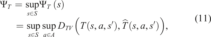
SNM is designed to address these issues. Instead of building upon existing non-linearity measures, SNM adopts approaches commonly used for sensitivity analysis (Mastin and Jaillet, 2012; Müller, 1997) of Markov Decision Processes (MDP)—a special class of POMDP where the observation model is perfect, and therefore the system is fully observable. These approaches use statistical distance measures between the original transition dynamics and their perturbed versions. Linearized dynamics can be viewed as a special case of perturbed dynamics, and hence this statistical distance measure can be applied as a non-linearity measure, too. We do need to extend these analyses, as they are generally defined for discrete state space and are defined with respect to only the transition models (MDP assumes the state of the system is fully observable). Nevertheless, such extensions are feasible and the generality of this measure could help to identify the effectiveness of linearization in motion planning under uncertainty problems.

3. Statistical-distance-based non-linearity measure (SNM)

Intuitively, our proposed measure SNM is based on the total variation distance between the effect of performing an action and perceiving an observation under the true dynamics and sensing model, and the effect under the linearized dynamic and sensing model. The total variation distance D _TV between two probability measures μ and ν over a measurable space Ω is defined as D _TV (μ,ν) = sup_E∈Ω|μ(E) − ν(E)|. An equivalent definition of D _TV which we use in our analysis is D _TV (μ,ν) = $\frac{1}{2}$ sup_|f|≤1|∫fdμ − ∫fdν| (Gibbs and Su, 2002). Formally, SNM is defined as

Definition 1

Let P = ⟨S, A, O, T, Z, R, b₀, γ⟩ be the POMDP model of the system and $\widehat{P}=〈S,A,O,\widehat{T},\widehat{Z},R,b_0,\gamma 〉$ be a linearization of P, where $\widehat{T}$ is a linearization of the transition function T and $\widehat{Z}$ is a linearization of the observation function Z of P, while all other components of P and $\widehat{P}$ are the same. Then, the SNM (denoted as Ψ) between P and $\widehat{P}$ is $\mathrm{\Psi }\left(P,\widehat{P}\right)={\mathrm{\Psi }}_T\left(P,\widehat{P}\right)+{\mathrm{\Psi }}_Z\left(P,\widehat{P}\right)$ , where

${\mathrm{\Psi }}_T\left(P,\widehat{P}\right)=\underset{s\in S,a\in A}{\sup }{D}_{TV}\left(T\left(s,a,s^{\prime }\right),\widehat{T}\left(s,a,s^{\prime }\right)\right),$

(3)

${\mathrm{\Psi }}_Z\left(P,\widehat{P}\right)=\underset{s^{\prime }\in S,a\in A}{\sup }{D}_{TV}\left(Z\left(s^{\prime },a,o\right),\widehat{Z}\left(s^{\prime },a,o\right)\right).$

(4)

Note that SNM can be applied as both a global and a local measure. In the latter case, the supremum over the state s can be restricted to a subset of S, rather than the entire state space. Furthermore, SNM is general enough for any approximation to the true dynamics and sensing model, which means that it can be applied to any type of linearization and belief approximation techniques, including those that assume and those that do not assume Gaussian belief simplifications.

We want to use the measure $\mathrm{\Psi }\left(P,\widehat{P}\right)$ to bound the difference between the expected total reward received if the system were to run the optimal policy of the true model P and if it were to run the optimal policy of the linearized model $\widehat{P}$ . Note that since our interest is in the actual reward received, the values of these policies are evaluated with respect to the original model P (we assume P is a faithful model of the system). More precisely, we want to show that:

Theorem 2

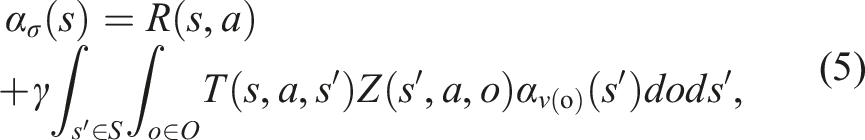
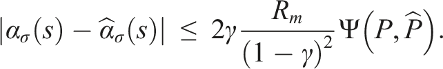
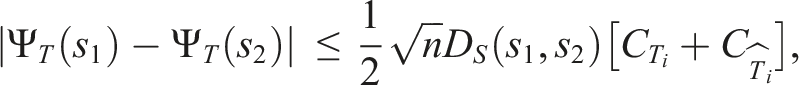
If π* denotes the optimal policy for P and ${\widehat{\pi }}^{*}$ denotes the optimal policy for $\widehat{P}$ , then for any $b\mathbb{\in }\mathbb{B}$ ,

$V_{\pi *}\left(b\right)-V_{{\widehat{\pi }}^{*}}\left(b\right)\le 4\gamma \frac{R_{max}}{{\left(1-\gamma \right)}^2}\mathrm{\Psi }\left(P,\widehat{P}\right),$

where V _π (b) = R(b, π(b)) + γ∫_o∈OZ(b, a, o)V _π (τ(b, a, o))do for any policy π and τ(b, a, o) is the belief transition function as defined in equation. (2).

To prove Theorem 2, we first assume, without loss of generality, that a policy π for a belief b is represented by a conditional plan σ ∈ Γ, where Γ is the set of all conditional plans. The plan σ can be specified by a pair 〈a,ν〉, where a ∈ A is the action of σ and ν: O → Γ is an observation strategy, which maps an observation to a conditional plan σ′ ∈ Γ.

Every σ corresponds to an α-function ${\alpha }_{\sigma }:S\to \mathbb{R}$ which specifies the expected total discounted reward the robot receives when executing σ starting from s ∈ S, that is

$\begin{array}{l}{\alpha }_{\sigma }\left(s\right)=R\left(s,a\right)\\ +\gamma {\int }_{s^{\prime }\in S}{\int }_{o\in O}T\left(s,a,s^{\prime }\right)Z\left(s^{\prime },a,o\right){\alpha }_{\nu \left(\mathrm{o}\right)}\left(s^{\prime }\right)dod{s}^{\prime },\end{array}$

(5)

where a ∈ A is the action of σ and α_ν(o) is the α-function corresponding to conditional plan ν(o).

For a given belief b, the value of the policy π represented by the conditional plan σ is then V _π (b) = ∫_s∈Sb(s)α _σ (s)ds. Note that equation (5) is defined with respect to POMDP P. Analogously, we define the linearized α-function ${\widehat{\alpha }}_{\sigma }$ with respect to the linearized POMDP $\widehat{P}$ by replacing the transition and observation functions in equation (5) with their linearized versions.

Now, suppose that for a given belief b, σ* = arg sup_σ∈Γ ∫_s∈Sb(s)α _σ (s)ds and $\widehat{\sigma }*={\text{arg\hspace{0.17em}sup}}_{\sigma \in \mathrm{\Gamma }}{\int }_{s\in S}b\left(s\right){\widehat{\alpha }}_{\sigma }\left(s\right)ds$ . The plans σ* and $\widehat{\sigma }*$ represent the policies π* and $\widehat{\pi }*$ that are optimal at b for POMDP P and $\widehat{P}$ , respectively. For any s ∈ S we have that ${\alpha }_{{\widehat{\sigma }}^{*}}\left(s\right)\ge {\alpha }_{{\widehat{\sigma }}^{*}}\left(s\right)-\left|{\alpha }_{{\widehat{\sigma }}^{*}}\left(s\right)-{\widehat{\alpha }}_{{\widehat{\sigma }}^{*}}\left(s\right)\right|$ and ${\widehat{\alpha }}_{\sigma *}\left(s\right)\ge {\alpha }_{\sigma *}\left(s\right)-\left|{\alpha }_{\sigma *}\left(s\right)-{\widehat{\alpha }}_{\sigma *}\left(s\right)\right|$ . Therefore

$\begin{array}{l}{\int }_{s\in S}b\left(s\right){\alpha }_{{\widehat{\sigma }}^{*}}\left(s\right)ds\ge {\int }_{s\in S}b\left(s\right){\widehat{\alpha }}_{{\widehat{\sigma }}^{*}}\left(s\right)ds\\ -{\int }_{s\in S}b\left(s\right)\left|{\alpha }_{{\widehat{\sigma }}^{*}}\left(s\right)-{\widehat{\alpha }}_{{\widehat{\sigma }}^{*}}\left(s\right)\right|ds,\end{array}$

(6)

and

$\begin{array}{l}{\int }_{s\in S}b\left(s\right){\widehat{\alpha }}_{{\widehat{\sigma }}^{*}}\left(s\right)ds\ge {\int }_{s\in S}b\left(s\right){\alpha }_{\sigma *}\left(s\right)ds\\ -{\int }_{s\in S}b\left(s\right)\left|{\alpha }_{\sigma *}\left(s\right)-{\widehat{\alpha }}_{\sigma *}\left(s\right)\right|ds.\end{array}$

(7)

Since ${\widehat{\sigma }}^{*}$ is the optimal conditional plan for POMDP $\widehat{P}$ at b, we also know that

${\int }_{s\in S}b\left(s\right){\widehat{\alpha }}_{{\widehat{\sigma }}^{*}}\left(s\right)ds\ge {\int }_{s\in S}b\left(s\right){\widehat{\alpha }}_{\sigma *}\left(s\right)ds.$

(8)

From equation. (6), equation. (7) and equation (8) it immediately follows that

$\begin{array}{l}{\int }_{s\in S}b\left(s\right){\alpha }_{{\widehat{\sigma }}^{*}}\left(s\right)ds\ge {\int }_{s\in S}b\left(s\right){\alpha }_{\sigma *}\left(s\right)ds\\ -2{\int }_{s\in S}b\left(s\right)\underset{\sigma \in \mathrm{\Gamma }}{\sup }\left|{\alpha }_{\sigma }\left(s\right)-{\widehat{\alpha }}_{\sigma }\left(s\right)\right|ds\\ V_{{\widehat{\pi }}^{*}}\left(b\right)\ge V_{\pi *}\left(b\right)\\ -2{\int }_{s\in S}b\left(s\right)\underset{\sigma \in \mathrm{\Gamma }}{\sup }\left|{\alpha }_{\sigma }\left(s\right)-{\widehat{\alpha }}_{\sigma }\left(s\right)\right|ds.\end{array}$

(9)

Before we continue, we first have to show the following Lemma:

Lemma 3

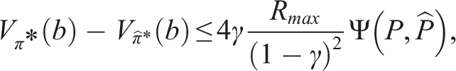
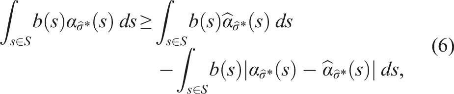
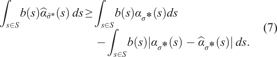
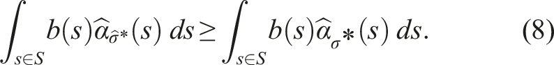
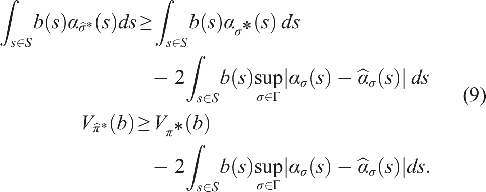
Let R _m = max{|R _min |,R _max }, where R _min = min_s,aR(s, a) and R _max = max_s,aR(s, a). For any conditional plan σ ∈ Γ and any s ∈ S, the absolute difference between the original and linearized α-functions is upper-bounded by

$\left|{\alpha }_{\sigma }\left(s\right)-{\widehat{\alpha }}_{\sigma }\left(s\right)\right|\le 2\gamma \frac{R_m}{{\left(1-\gamma \right)}^2}\mathrm{\Psi }\left(P,\widehat{P}\right).$

The proof of Lemma 3 is presented in Appendix A.1. Using the result of Lemma 3, we can now conclude the proof for Theorem 2. Substituting the upper bound derived in Lemma 3 into the right-hand side of equation (9) and re-arranging the terms gives us

$V_{\pi *}\left(b\right)-V_{{\widehat{\pi }}^{*}}\left(b\right)\le 4\gamma \frac{R_m}{{\left(1-\gamma \right)}^2}\mathrm{\Psi }\left(P,\widehat{P}\right),$

(10)

which is what we are looking for.

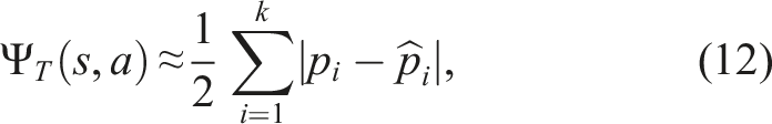
4. Approximating SNM

Ultimately, we want to use SNM as a heuristic during online planning to decide when a linearization-based solver will likely yield a good policy and when a general solver should be used. However, computing SNM exactly is challenging, due to having to find the suprema over the state and action spaces in equation. (3) and equation. (4). Here, we provide an efficient approximation algorithm to estimate SNM. We focus on approximating the transition component Ψ _T of SNM. The observation component Ψ _Z is approximated similarly.

Let us first rewrite the transition component of Ψ _T as

$\begin{array}{l}{\mathrm{\Psi }}_T=\underset{s\in S}{\sup }{\mathrm{\Psi }}_T\left(s\right)\\ =\underset{s\in S}{\sup }\underset{a\in A}{\sup }{D}_{TV}\left(T\left(s,a,s^{\prime }\right),\widehat{T}\left(s,a,s^{\prime }\right)\right),\end{array}$

(11)

where Ψ _T (s) is the transition component of SNM, given a particular state. To approximate Ψ _T , we replace S in equation (11) by a sampled representation of S, which we denote as $\stackrel{\sim }{S}$ . The value Ψ _T (s) is then evaluated for each $s\in \stackrel{\sim }{S}$ offline, and the results are saved in a lookup-table. This lookup-table can then be used during run-time to get a local approximation of Ψ _T around the current belief.

To construct $\stackrel{\sim }{S}$ efficiently, we assume the problem is deterministic and use kinodynamic RRT (Kuffner and LaValle, 2011) to solve the resulting motion planning problem. RRT constructs a space-filling tree in the state space, thus, we can use the nodes to form $\stackrel{\sim }{S}$ . Note that RRT generates states according to a deterministic transition function only. If required, one could also generate additional samples according to the actual stochastic transition function of the robot. However, in our experiments, the state samples generated by RRT were sufficient.

To approximate the supremum over the action space in equation (11), we discretize the action space, leaving us with a maximization problem over discrete actions, denoted as $\stackrel{\sim }{A}$ . Given $\stackrel{\sim }{A}$ , we approximate Ψ _T (s, a) for each $s\in \stackrel{\sim }{S}$ and $a\in \stackrel{\sim }{A}$ by drawing n samples from the original and linearized transition function and construct a multidimensional histogram from both sample sets. Suppose the histogram consists of k bins. The value Ψ _T (s, a) is then approximated as

${\mathrm{\Psi }}_T\left(s,a\right)\approx \frac{1}{2}{\displaystyle \sum }_{i=1}^k\left|p_i-{\widehat{p}}_i\right|,$

(12)

where $p_i=n_i/{\sum }_{j=1}^k{n}_j$ and n _i is the number of states inside bin i sampled from the original transition function, while ${\widehat{p}}_i={\widehat{n}}_i/{\sum }_{j=1}^k{\widehat{n}}_j$ and ${\widehat{n}}_i$ is the number of states inside bin i sampled from the linearized transition function. Note that the right-hand side of equation (12) is simply the definition of the total variation distance between two discrete distributions. Given a particular state $s\in \stackrel{\sim }{S}$ , we maximize equation (12) with respect to $\stackrel{\sim }{A}$ , which gives us an approximation of Ψ _T (s). Repeating this process for every $s\in \stackrel{\sim }{S}$ results in a lookup-table, which assigns each state $s\in \stackrel{\sim }{S}$ an approximated value of Ψ _T (s).

During planning, we can use the lookup-table and a sampled representation of a belief b to approximate SNM at b. Suppose $\stackrel{\sim }{b}$ is the sampled representation of b, for example, a particle set. Then, for each state $s\in \stackrel{\sim }{b}$ , we take the state $s_{near}\in {\stackrel{\sim }{S}}_{b_0}$ that is closest to s, and assign Ψ _T (s) = Ψ _T (s _near ). The maximum SNM value ${\max }_{s\in \stackrel{\sim }{b}}\hspace{0.17em}{\mathrm{\Psi }}_T\left(s\right)$ gives us an approximation of the transition component of SNMwith respect to the belief b.

The above approximation method assumes that states that are close together should yield similar values for SNM. At a first glance, this is a very strong assumption. In the vicinity of obstacles or constraints, states that are close together could potentially yield very different SNM-values. However, we will now show that under mild assumptions, pairs of states that are elements within certain subsets of the state space indeed yield similar SNM-values.

Consider a partitioning of the state space into a finite number of local-Lipschitz subsets S _i that are defined as follows:

Definition 4

Let S be a metric space with distance metric D _S . S _i is called a local-Lipschitz subset of S if for any s₁, s₂ ∈ S _i , any s′ ∈ S and any $a\in A:\left|T\left(s_1,a,s^{\prime }\right)-T\left(s_2,a,s^{\prime }\right)\right|\le C_{T_i}{D}_S\left(s_1,s_2\right)$ and $\left|\widehat{T}\left(s_1,a,s^{\prime }\right)-\widehat{T}\left(s_2,a,s^{\prime }\right)\right|\le C_{{\widehat{T}}_i}{D}_S\left(s_1,s_2\right)$ , where $C_{T_i}\ge 0$ and $C_{{\widehat{T}}_i}\ge 0$ are finite local-Lipschitz constants

In other words, S _i are subsets of S in which the original and linearized transition functions are Lipschitz continuous with Lipschitz constants $C_{T_i}$ and $C_{{\widehat{T}}_i}$ . With this definition at hand, we can now show the following lemma:

Lemma 5

Let S be a n − dimensional metric space with distance metric D _S and assume S is normalized to [0,1] ⁿ . Furthermore, let S _i be a local-Lipschitz subset of S, then

$\left|{\mathrm{\Psi }}_T\left(s_1\right)-{\mathrm{\Psi }}_T\left(s_2\right)\right|\le \frac{1}{2}\sqrt{n}{D}_S\left(s_1,s_2\right)\left[C_{T_i}+C_{{\widehat{T}}_i}\right],$

for any s₁, s₂ ∈ S _i

The proof for this Lemma is presented in Appendix A.2. This Lemma indicates that the difference between the SNM-values for two states from the same local-Lipschitz subset S _i depends only on the distance D _S between them, since $C_{T_i}$ and $C_{{\widehat{T}}_i}$ are constant for each subset S _i . Thus, as the distance between two states converges towards zero, the SNM value difference converges towards zero as well. This implies that we can approximate SNM for a sparse, sampled representation of $S_{b_0}$ and re-use these approximations online with a small error, without requiring an explicit representation of the S _i subsets.

5. SNM-planner: An application of SNM for planning

SNM-Planner is an online planner that uses SNM as a heuristic to decide whether a general, or a linearization-based POMDP solver should be used to compute the policy from the current belief. The general solver used is Adaptive Belief Tree (ABT) (Kurniawati and Yadav, 2016), while the linearization-based method called Modified High-Frequency Replanning (MHFR), which is an adaptation of HFR (Sun et al., 2015). HFR is designed for chance-constraint POMDPs, that is, it explicitly minimizes the collision probability, while MHFR is a POMDP solver where the objective is to maximize the expected total reward. An overview of SNM-Planner is shown in Algorithm 1. During run-time, at each planning step, SNM-Planner computes a local approximation of SNM around the current belief b (line 5). If this value is smaller than a given threshold, SNM-Planner uses MHFR to compute a policy from the current belief, whereas ABT is used when the value exceeds the threshold (lines 7 to 11). The robot then executes an action according to the computed policy (line 12) and receives an observation (line 13). Based on the executed action and perceived observation, we update the belief (line 14). SNM-Planner represents beliefs as sets of particles and updates the belief using a SIR particle filter (Arulampalam et al., 2002). Note that MHFR assumes that beliefs are multivariate Gaussian distributions. Therefore, in case MHFR is used for the policy computation, we compute the first two moments (mean and covariance) of the particle set to obtain a multivariate Gaussian approximation of the current belief. The process then repeats from the updated belief until the robot has entered a terminal state (we assume that we know when the robot enters a terminal state).

In the following two subsections we provide a brief an overview of the two component planners ABT and MHFR.

Algorithm 1 SNM-Planner (initial belief b₀, SNM threshold μ, max. planning time per step t)

1: Initialize ABT(P)

2: Initialize MHFR(P)

3: b = b0, terminal = False

4: while terminal is False do

5:   $\widehat{\mathrm{\Psi }}=$ approximate SNM(b)

6:  t p = t − t a ⊳ t a is the time the algorithm takes to approximate SNM

7:  if $\widehat{\mathrm{\Psi }}<\mu$ then

8:   a = MHFR(b i , t p )

9:  else

10:  a = ABT(b i , t p )

11:  end if

12:  terminal = execute Action(a)

13:  o = get observation

14:  b′ = τ(b, a, o)

15:  b = b′

16: end while

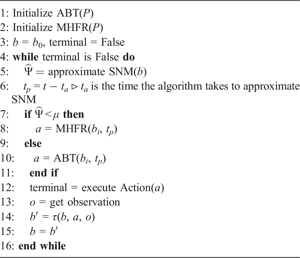
5.1. Adaptive belief tree (ABT)

ABT is a general and anytime online POMDP solver based on Monte-Carlo-Tree-Search (MCTS). ABT updates (rather than recomputes) its policy at each planning step. To update the policy for the current belief, ABT iteratively constructs and maintains a belief tree, a tree whose nodes are beliefs and whose edges are pairs of actions and observations. ABT evaluates sequences of actions by sampling episodes, that is, sequences of state—action—observation—reward tuples, starting from the current belief. Details of ABT can be found in Kurniawati and Yadav (2016).

5.2. Modified high-frequency replanning (MHFR)

The main difference between HFR and MHFR is that HFR is designed for chance-constraint POMDP, that is, it explicitly minimizes the collision probability, while MHFR is a POMDP solver, whose objective is to maximize the expected total reward. Similar to HFR, MHFR approximates the current belief by a multivariate Gaussian distribution. To compute the policy from the current belief, MHFR samples a set of trajectories from the mean of the current belief to a goal state using multiple instances of RRTs (Kuffner and LaValle, 2011) in parallel. It then computes the expected total discounted reward of each trajectory by tracking the beliefs around the trajectory using a Kalman Filter, assuming maximum-likelihood observations. The policy then becomes the first action of the trajectory with the highest expected total discounted reward. After executing the action and perceiving an observation, MHFR updates the belief using an Extended Kalman Filter. The process then repeats from the updated belief. To increase efficiency, MHFR additionally adjusts the previous trajectory with the highest expected total discounted reward to start from the mean of the updated belief and adds this trajectory to the set of sampled trajectories. More details on HFR and precise derivations of the method are available in Sun et al. (2015).

6. Experiments and results

The purpose of our experiments is two-fold: To test the applicability of SNM to motion planning under uncertainty problems and to test SNM-Planner. For our first objective, we compare SNM with a modified version of the Measure of Non-Gaussianity (MoNG) (Duník et al., 2013). Details regarding MoNG are provided in Section 6.1. We evaluate both measures using two simulated robotic systems, a car-like robot with 2 ^nd -order dynamics and a torque-controlled 4DOFs manipulator, where both robots are subject to increasing uncertainties and increasing numbers of obstacles in the operating environment. The selected robotic systems are commonly used to evaluate linearization-based solvers (van Den Berg et al., 2011; Sun et al., 2015; Prentice and Roy, 2009). Furthermore, we test both measures when the robots are subject to highly non-linear collision dynamics and different observation models. Details on the robot models are presented in Section 6.2, whereas the evaluation experiments are presented in Section 6.3.

To test SNM-Planner, we compare it with ABT and MHFR on four problem scenarios, including a torque-controlled 7DOFs manipulator operating inside a 3D office environment, and a 7DOFs velocity controlled manipulator working collaboratively with a human worker on a factory control terminal. Additionally, we test how sensitive SNM-Planner is to the choice of the SNM-threshold. The results for these experiments are presented in Section 6.4.

All problem environments are modeled within the OPPT framework (Hoerger et al., 2018). The solvers are implemented in C++. All simulations were run on an AMD EPYC 7003 CPU with 8 GB of memory. For the parallel construction of the RRTs in MHFR, we utilize 8 CPU cores throughout the experiments. All parameters are set based on preliminary runs over the possible parameter space, the parameters that generate the best results are then chosen to generate the experimental results.

6.1. Measure of non-gaussianity

The Measure of Non-Gaussianity (MoNG) proposed in Duník et al. (2013) is based on the negentropy between the PDF of a random variable and its Gaussian approximation. Consider a n-dimensional random variable X distributed according to PDF p(x). Furthermore, let $\widehat{X}$ be a Gaussian approximation of X with PDF $\widehat{p}\left(x\right)$ , such that $\widehat{X}\sim N\left(\mu ,{\mathrm{\Sigma }}_x\right)$ , where μ and Σ _x are the first two moments of p(x). The negentropy between p and $\widehat{p}$ (denoted as $J\left(p,\widehat{p}\right)$ ) is then defined as

$J\left(p,\widehat{p}\right)=H\left(\widehat{p}\right)-H\left(p\right),$

(13)

where

$\begin{array}{l}H\left(\widehat{p}\right)=\frac{1}{2}\ln \left({\left(2\pi e\right)}^n\left|\det \left({\mathrm{\Sigma }}_x\right)\right|\right),\\ H\left(p\right)=-\int p\left(x\right)\ln \hspace{0.17em}p\left(x\right)dx\end{array}$

(14)

are the differential entropies of p and $\widehat{p}$ , respectively. A (multivariate) Gaussian distribution has the largest differential entropy amongst all distributions with equal first two moments, therefore $J\left(p,\widehat{p}\right)$ is always non-negative. In practice, since the PDF p(x) is not known exactly in all but the simplest cases, H(p) has to be approximated.

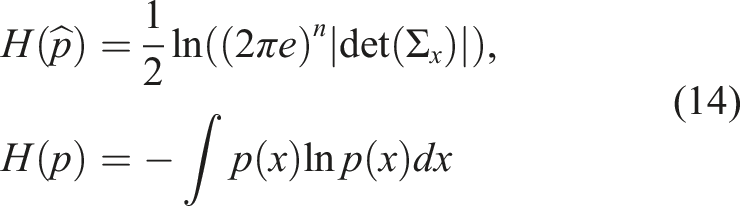
In Duník et al. (2013) this measure has originally been used to assess the non-linearity of passive systems. Therefore, in order to achieve comparability with SNM, we need to extend the Non-Gaussian measure to general active stochastic systems of the form s_t+1 = f (s _t , a _t , v _t ). We do this by evaluating the non-Gaussianity of distribution that follow from the transition function T(s, a, s′) given state s and action a. In particular, for a given s and a, we can find a Gaussian approximation of T(s, a, s′) (denoted by T _G (s, a, s′)) by calculating the first two moments of the distribution that follows from T(s, a, s′).

Using this Gaussian approximation, we define the Measure of Non-Gaussianity as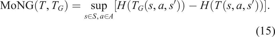

$\text{MoNG}\left(T,T_G\right)=\underset{s\in S,a\in A}{\sup }\left[H\left(T_G\left(s,a,s^{\prime }\right)\right)-H\left(T\left(s,a,s^{\prime }\right)\right)\right].$

(15)

Similarly, we can compute the Measure of Non-Gaussianity for the observation function:

$\text{MoNG}\left(Z,Z_G\right)=\underset{s\in S,a\in A}{\sup }\left[H\left(Z_G\left(s^{\prime },a,o\right)\right)-H\left(Z\left(s^{\prime },a,o\right)\right)\right],$

(16)

where Z _G is a Gaussian approximation of Z.

In order to approximate the entropies H(T(s, a, s′))) and H(Z(s′, a, o)), we are using a similar histogram-based approach as discussed in Section 4. The entropy terms for the Gaussian approximations can be computed in closed form, according to the first equation in equation (14) (Ahmed and Gokhale, 1989).

6.2. Robot models

6.2.1. 4DOFs manipulator

The 4DOFs manipulator consists of 4 links connected by 4 torque-controlled revolute joints. The first joint is connected to a static base. In all problem scenarios, the manipulator must move from a known initial state to a state where the end-effector lies inside a goal region located in the workspace of the robot, while avoiding collisions with obstacles the environment is populated with.

The state of the manipulator is defined as $s=\left(\theta ,\stackrel{.}{\theta }\right)\in {\mathbb{R}}^8$ , where θ is the vector of joint angles, and $\stackrel{.}{\theta }$ the vector of joint velocities. Both joint angles and joint velocities are subject to linear constraints: The joint angles are constrained by (−3.14, 3.14)rad, whereas the joint velocities are constrained by (6, 2, 2, 2)rad/s in each direction. Each link of the robot has a mass of 1 kg.

The control inputs of the manipulator are the joint torques, where the maximum joint torques are (20, 20, 10, 5)Nm/s in each direction. Since ABT assumes a discrete action space, we discretize the joint torques for each joint using the maximum torque in each direction, which leads to 16 actions.

The dynamics of the manipulator is defined using the well-known Newton-Euler formalism (Spong et al., 2006). For both manipulators, we assume that the input torque for each joint is affected by zero-mean additive Gaussian noise. Note however, even though the error is Gaussian, due to the non-linearities of the motion dynamics the beliefs will not be Gaussian in general. Since the transition dynamics for this robot are quite complex, we assume that the joint torques are applied for 0.1s, and we use the ODE physics engine (Drumwright et al., 2010) for the numerical integration of the dynamics, where the discretization (i.e., δt) of the integrator is set to δt = 0.004s.

The robot is equipped with two sensors: The first sensor measures the position of the end-effector inside the robot’s workspace, whereas the second sensor measures the joint velocities. Consider a function $g:{\mathbb{R}}^8\mapsto {\mathbb{R}}^3$ that maps the state of the robot to an end-effector position inside the workspace, then the observation model is defined as

$o={\left[g\left(s\right),\stackrel{.}{\theta }\right]}^T+w,$

(17)

where w _t is an error term drawn from a zero-mean multivariate Gaussian distribution with covariance matrix Σ _w .

The initial state of the robot is a state where the joint angles and velocities are zero.

When the robot performs an action where it collides with an obstacle, it enters a terminal state and receives a penalty of −500. When it reaches the goal area, it also enters a terminal state, but receives a reward of 1000. To encourage the robot to reach the goal area quickly, it receives a small penalty of −1 for every other action.

6.2.2. 7DOFs Kuka iiwa manipulator

The 7DOFs Kuka iiwa manipulator is very similar to the 4DOFs manipulator. However, the robot consists of 7 links connected via 7 revolute joints. We set the POMDP model to be similar to that of the 4DOFs manipulator, but expand it to handle 7DOFs. For this robot, the joint velocities are constrained by (3.92, 2.91, 2.53, 2.23, 2.23, 2.23, 1.0)rad/s in each direction and the link masses are (4, 4, 3, 2.7, 1.7, 1.8, 0.3)kg. Additionally, the torque limits of the joints are (25, 20, 10, 10, 5, 5, 0.5)Nm/s in each direction. For ABT, we use the same discretization of the joint torques as in the 4DOFs manipulator case, that is, we use the maximum torque per joint in each direction, resulting in 128 actions. Similarly to the 4DOFs manipulator, we assume that the input torques are applied for 0.1s, and we use the ODE physics engine with an integration step size of 0.004s to simulate the transition dynamics. The observation and reward models are the same as for the 4DOFs manipulator. The initial joint velocities are all zero and almost all joint angles are zero too, except for the second joint, for which the initial joint angle is −1.5rad. Figure 1(c) shows the Kuka manipulator operating inside an office scenario.

Figure 1.

Test scenarios for the different robots. The objects colored black and gray are obstacles, while the green sphere is the goal region. (a) The Maze scenario for the car-like robot. The blue squares represent the beacons, while the orange square at the bottom left represents the initial state. (b) The 4DOFs manipulator scenario. (c) The KukaOffice scenario. (d) The JacoCollab scenario.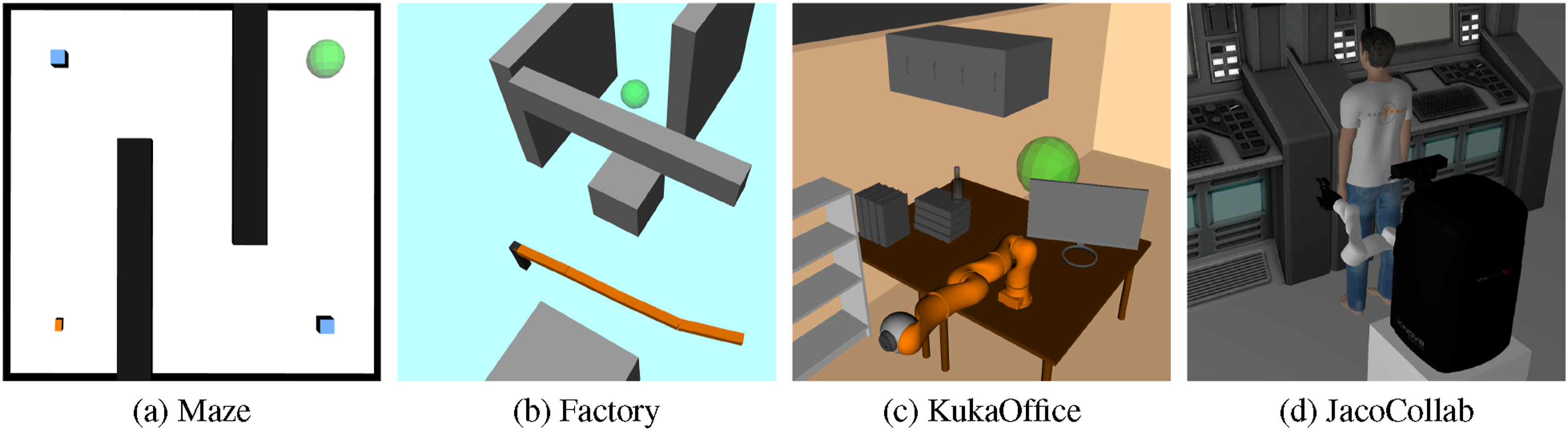

6.2.3. JacoCollab

The third robot we consider is a 7DOFs Jaco arm mounted on a fixed base, as shown in Figure 1(d). The robot consists of 7 links connected via revolute joints. In addition to the arm, the robot is equipped with a RGB-camera that is mounted on the base. The robot operates inside a control room in a factory, which consists of a control terminal located in front of the robot. In addition, a human worker moves around in front of the terminal, operating it collaboratively with the robot. In particular, we assume that the worker is located at x = 1m in front of the robot and moves along the y-axis of the robot’s base frame. However, the worker is not used to collaborate with a robot, and their motion becomes more erratic as their distance to the robot decreases. The goal of the robot is to reach the terminal with its end-effector, without colliding with the worker.

Here, the state space is defined as S = Θ × Y, where Θ is the set of all joint angles, and $Y=\mathbb{R}$ is the set of all positions of the worker along the y-axis of the robot’s base frame. The robot is controlled via a constant end-effector velocity of 5 cm/s in each of the ± x, ±y, ±z-directions (with respect to the robot’s base frame), resulting in six actions. At each step, an end-effector velocity command is applied for 1s and mapped to a joint-velocity command via an internal controller. While the dynamics of the robot are deterministic, the motion of the worker is uncertainty. In particular, we assume that the worker’s y-position evolves according to y_t+1 = y _t + e _T , with e _T ∼ U[-u _t , u _t ], where U is a uniform distribution over the interval [-u _t , u _t ]. The bound u _t depends on the closest Euclidean distance d _t between the robot and the worker at time t and is set to u _t =max{0.01,1/100d _t }. In other words, as the robot approaches the worker, their motion becomes more uncertain.

While the exact position of the worker is only partially observed, the robot can estimate it using its onboard camera. We use a simplified observation model and assume that the robot receives observations regarding the worker’s y-position according to o _t = y _t + e _Z , where e _Z ∼ U[−0.038, 0.038].

The robot receives a reward of 100 for reaching the control terminal with its end-effector. Upon collision with the worker, the robot receives a penalty of −100. Both events lead to a terminal state. Additionally, the robot receives a penalty of −1 for every step to encourage it to reach the control terminal quickly. The initial configuration and y-position of the worker are fully known and set to θ = (−0.37, 2.11, 0.29, 2.59, 0.54, 0.51, 1.62)rad and y = 0.2 m, respectively. The discount factor is γ = 0.99.

To reach the control terminal, the robot must act strategically by considering the behavior of the worker. Getting too close to the worker might lead to collisions, due to the increased uncertainty in the worker’s motion, while waiting too long for the worker to move out of the way leads to an increased time to reach the control terminal.

6.2.4. Car-like robot

A non-holonomic car-like robot of size (0.12 × 0.07 × 0.01) drives on a flat xy-plane inside a 3D environment populated by obstacles. The robot must drive from a known start state to a position inside a goal region without colliding with any of the obstacles. The state of the robot at time t is defined as a 4D vector $s_t=\left(x_t,y_t,{\theta }_t,{\upsilon }_t\right)\in {\mathbb{R}}^4$ , where x _t , y _t ∈ [−1, 1] is the position of the center of the robot on the xy-plane, θ _t ∈ [−3.14, 3.14]rad the orientation and υ _t ∈ [−0.2, 0.2] is the linear velocity of the robot. The initial state of the robot is (−0.7, − 0.7, 1.57 rad, 0) while the goal region is centered at (0.7, 0.7) with radius 0.1. The control input at time t, a _t = (α _t , ϕ _t ) is a 2D real vector consisting of the acceleration α ∈ [−1, 1] and the steering wheel angle ϕ _t ∈ [−1 rad, 1 rad]. The robot’s dynamics are subject to control noise $v_t=\left({\stackrel{\sim }{\alpha }}_t,{\stackrel{\sim }{\varphi }}_t\right)\sim N\left(0,{\mathrm{\Sigma }}_v\right)$ . The robot’s transition model is

$s_{t+1}=f\left(s_t,a_t,v_t\right)=\left[\begin{array}{c}{x}_t+\mathrm{\Delta }t{\upsilon }_t\hspace{0.17em}\cos \hspace{0.17em}{\theta }_t\\ y_t+\mathrm{\Delta }t{\upsilon }_t\hspace{0.17em}\sin \hspace{0.17em}{\theta }_t\\ {\theta }_t+\mathrm{\Delta }t\hspace{0.17em}\tan \left({\varphi }_t+{\stackrel{\sim }{\varphi }}_t\right)/0.11\\ {\upsilon }_t+\mathrm{\Delta }t\left({\alpha }_t+{\stackrel{\sim }{\alpha }}_t\right)\end{array}\right],$

(18)

where Δt = 0.3s is the duration of a time step and the value 0.11 is the distance between the front and rear axles of the wheels.

This robot is equipped with two types of sensors, a localization sensor that receives a signal from two beacons that are located at $\left({\widehat{x}}_1,{\widehat{y}}_1\right)$ and $\left({\widehat{x}}_2,{\widehat{y}}_2\right)$ . The second sensor is a velocity sensor mounted on the car. With these two sensors, the observation model is defined as

$o_t=\left[\begin{array}{c}\frac{1}{\left({\left(x_t-{\widehat{x}}_1\right)}^2+{\left(y_t-{\widehat{y}}_1\right)}^2+1\right)}\\ \frac{1}{\left({\left(x_t-{\widehat{x}}_2\right)}^2+{\left(y_t-{\widehat{y}}_2\right)}^2+1\right)}\\ v_t\end{array}\right]+w_t,$

(19)

where w _t is an error vector drawn from a zero-mean multivariate Gaussian distribution with covariance matrix Σ _w .

Similar to the manipulators described above, the robot receives a penalty of −500 when it collides with an obstacle, a reward of 1000 when reaching the goal area and a small penalty of −1 for any other action.

6.3. Testing SNM

In this set of experiments, we want to understand the performance of SNM compared to MoNG in various scenarios. In particular, we are interested in the effect of increasing uncertainties and the effect that obstacles have on the effectiveness of SNM, and if these results are consistent with the performance of a general solver relative to a linearization-based solver. Additionally, we want to see how highly non-linear collision dynamics and different observation models—one with additive Gaussian noise and non-additive Gaussian noise—affect our measure. For the experiments with increasing motion and sensing errors, recall from Section 6.2 that the control errors are drawn from zero-mean multivariate Gaussian distributions with covariance matrices Σ _v . We define the control errors (denoted as e _T ) to be the standard deviation of these Gaussian distributions, such that ${\mathrm{\Sigma }}_v={e_T}^2\times 1$ . Similarly, for the covariance matrices of the zero-mean multivariate Gaussian sensing errors, we define the observation error as e _Z , such that ${\mathrm{\Sigma }}_w={e_Z}^2\times 1$ . Note that during all the experiments, we use normalized spaces, which means that the error vectors affect the normalized action and observation vectors. For SNMand MoNGwe first generated 100,000 state samples for each scenario, and computed a lookup-table for each error value offline, as discussed in Section 4. Then, during run-time, we calculated the average approximated SNM and MonG values.

6.3.1. Effects of increasing uncertainties in cluttered environments

To investigate the effect of increasing control and observation errors on SNM, MoNG and the two solvers ABT and MHFR in cluttered environments, we ran a set of experiments where the 4DOFs manipulator and the car-like robot operate in empty environments, environments with obstacles, and environments where the robots interact with the environment via collision dynamics with increasing values of e _T and e _Z , ranging between 0.001 and 0.075. For the last set of environments, the robots are allowed to collide with the obstacles, that is, a collision does not result in a terminal state. The dynamics effects of collisions are reflected in the transition model. In particular, for the 4DOFs manipulator, collisions are modeled as additional constraints (contact points) that are resolved by applying “correcting velocities” to the colliding bodies in the opposite direction of the contact normals. For the car-like robot, we modify the transition model equation (18) to consider collision dynamics such that

$s_{t+1}=\{\begin{array}{ll}{f}_{col}\left(s_t,a_t,v_t\right)& \text{if}\hspace{0.17em}f\left(s_t,a_t,v_t\right)\hspace{0.17em}\text{collides},\\ f\left(s_t,a_t,v_t\right)& \text{else},\end{array}$

(20)

where

$f_{coll}\left(s_t,a_t,v_t\right)={\left[x_t,y_t,{\theta }_t,-3v_t\right]}^T.$

(21)

This transition function causes the robot to slightly “bounce” off obstacles upon collision.

The environments with obstacles (both with and without collision dynamics) are the Factory and Maze environments shown in Figure 1(a) and (b). For each scenario and each control-sensing error value (we set e _T = e _Z ), we ran 100 simulation runs using ABT and MHFR, respectively, with a planning time of 2s per step.

Figures 2 and 3 show the average values of SNM and MoNG and the relative value differences between ABT and MHFR for the 4DOFs manipulator and the car-like robot, respectively. The results show that in empty environments, both SNM and MoNG are sensitive to increasing transition and observation errors. This resonates well with the relative value difference between ABT and MHFR. However, for environments with obstacles and environments with collision dynamics, SNM increases significantly compared to the empty environments, whereas MoNG remains almost unaffected in the Factory and Maze environments and only increases marginally as collision dynamics are introduced. Overall, the added non-linearities introduced by obstacles and collision dynamics increase the value difference between ABT and MHFR, except for large uncertainties in the Maze environment. This indicates that MHFR suffers more from the added non-linearities compared to ABT. SNMis able to capture these effects much better compared to MoNG.

Figure 2.

Evaluations of the tested measures and the relative value difference between ABT and MHFR for the 4DOFs manipulator operating in an empty environment (red lines), the Factory environment (green lines) and the Factory environment with collision dynamics (blue lines). (a) The average values of SNM as the transition (e _T ) and observation (e _Z ) errors increase. (b) The average values of MoNG as the transition and observation errors increase. (c) The relative value difference between ABT and MHFR as the transition and observation errors increase.

Figure 3.

Evaluations of the tested measures and the relative value difference between ABT and MHFR for the Car-like robot operating in an empty environment (red lines), the Maze environment (green lines) and the Maze environment with collision dynamics (blue lines). (a) The average values of SNM as the transition (e _T ) and observation (e _Z ) errors increase. (b) The average values of MoNG as the transition and observation errors increase. (c) The relative value difference between ABT and MHFR as the transition and observation errors increase.

An interesting remark regarding the results for the Maze scenario in Figure 3(c) is that the relative value difference actually decreases for large uncertainties. The reason for this can be seen in Figure 4. As the uncertainties increase, the problem becomes so difficult, such that both solvers fail to compute a reasonable policy within the given planning time. However, clearly, MHFR suffers earlier from these large uncertainties compared to ABT.

Figure 4.

The average total discounted rewards achieved by ABT and MHFR in the Maze scenario, as the uncertainties increase. Vertical bars are the 95% confidence intervals.

6.3.2. Effects of increasingly cluttered environments

To investigate the effects of increasingly cluttered environments on SNM and MoNG, we ran a set of experiments in which the car-like robot and the 4DOFs manipulator operate inside environments with an increasing number of randomly distributed obstacles. For this we generated test scenarios with 5, 10, 15, 20, 25 and 30 obstacles that are uniformly distributed across the environment. For each of these test scenarios, we randomly generated 100 environments. Figure 5 shows two example environments with 30 obstacles for the Car-like robot and the 4DOFs manipulator. For this set of experiments, we do not take collision dynamics into account. The control and observation errors are fixed to e _t = e _z = 0.038 which corresponds to the median of the uncertainty values.

Figure 5.

Two example scenarios for the Car-like robot (a) and the 4DOFs manipulator (b) with 30 randomly distributed obstacles.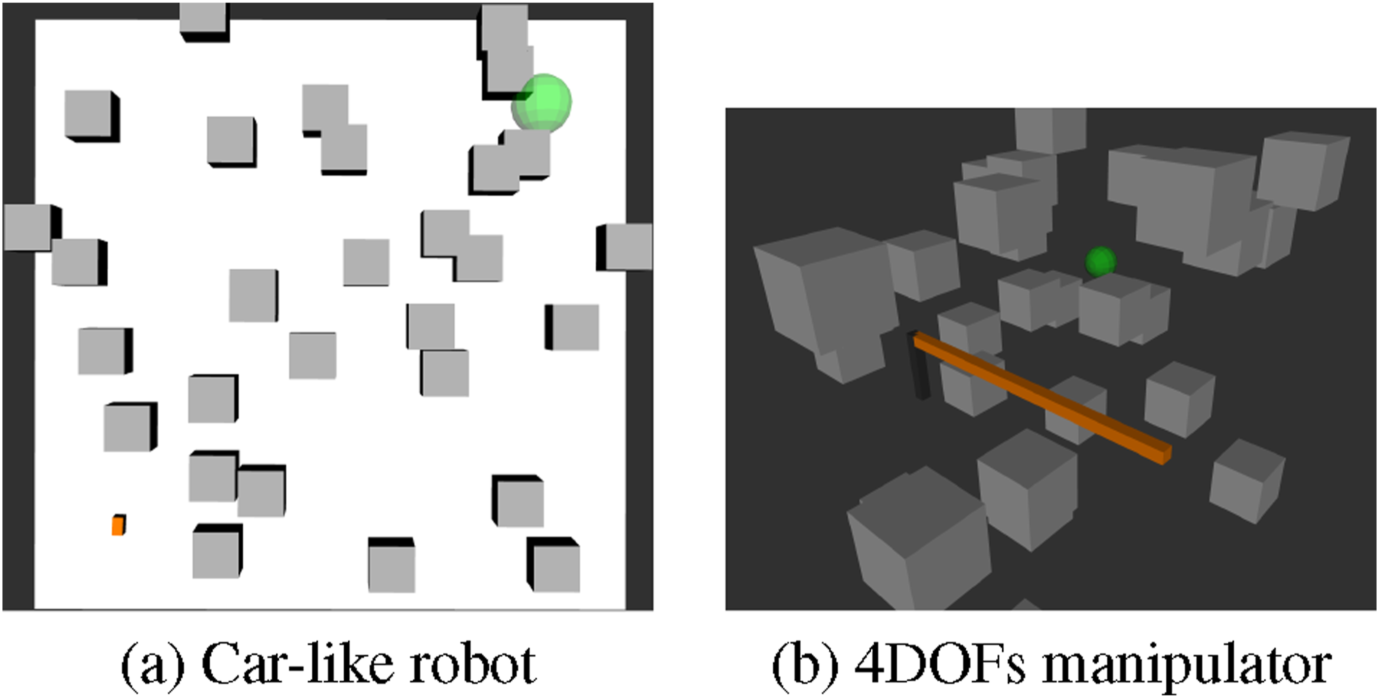

Figure 6 presents the results for SNM, MoNG and the relative value difference between ABT and MHFR for the 4DOFs manipulator (top row) and the car-like robot (bottom row). From these results it is clear that, as the environments become increasingly cluttered, the advantage of ABT over MHFR increases, indicating that the obstacles have a significant effect on the Gaussian belief assumption of MHFR. Additionally, SNM is clearly more sensitive to those effects compared to MoNG, whose values remain virtually unaffected by the amount of clutter in the environments.

Figure 6.

Evaluations of the tested measures and the relative value difference between ABT and MHFR on the 4DOFs manipulator (top row) and the Car-like robot (bottom row) operating in environments with increasing numbers of obstacles. (a) The average values of SNM (red line) and MoNG (blue line) for the 4DOFs manipulator operating inside environments with increasing numbers of obstacles. (b) The relative value difference between ABT and MHFR for the 4DOFs manipulator operating in environments with increasing numbers of obstacles. (c) The average values of SNM(red line) and MoNG (blue line) for the Car-like robot operating inside environments with increasing numbers of obstacles. (d) The relative value difference between ABT and MHFR for the Car-like robot operating inside environments with increasing numbers of obstacles.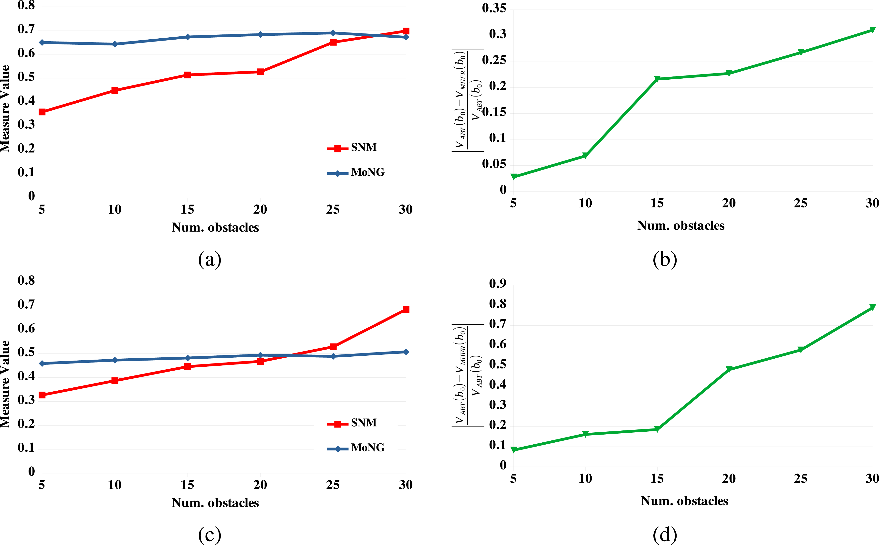

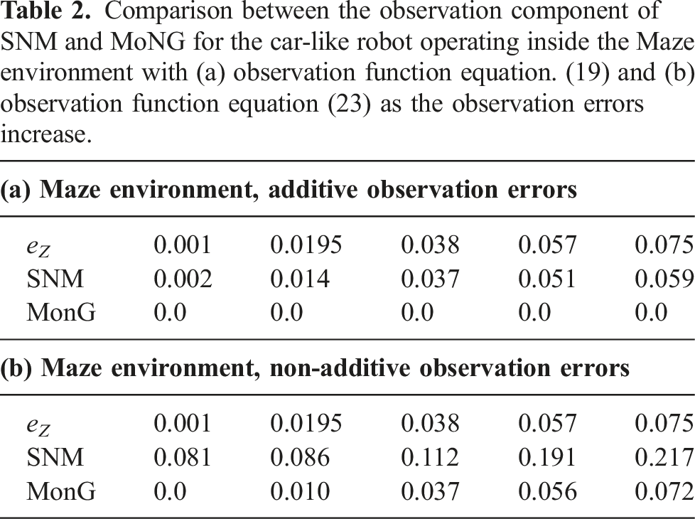
6.3.3. Effects of non-linear observation functions with non-additive errors

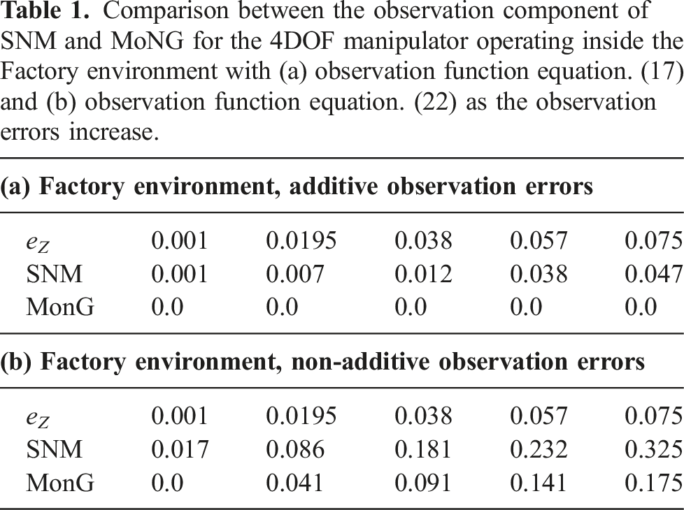
In the previous experiments, we assumed that the observation functions are non-linear functions with additive Gaussian noise, a special class of non-linear observation functions. This class of observation functions has some interesting implications: First, the resulting observation distribution remains Gaussian. This in turn means that MoNG for the observation function evaluates to zero. Second, linearizing the observation function results in a Gaussian distribution with the same mean but different covariance. We therefore expect that the observation component SNM remains small, even for large uncertainties. To investigate how SNM reacts to non-linear observation functions with non-additive noise, we ran a set of experiments for the 4DOFs manipulator operating inside the Factory environment and the car-like robot operating inside the Maze environment where we replaced both observation functions with non-linear functions with non-additive noise. For the 4DOFs manipulator, we replaced the observation function defined in equation (17) with

$o_t=g\left(s_t+w_t\right),$

(22)

where w _t ∼ N(0, Σ _w ). In other words, the manipulator has only access to a sensor that measure the position of the end-effector in the workspace.

For the car-like robot, we use the following observation function: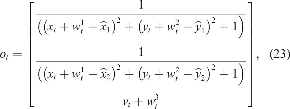

$o_t=\left[\begin{array}{c}\frac{1}{\left({\left(x_t+w_t^1-{\widehat{x}}_1\right)}^2+{\left(y_t+w_t^2-{\widehat{y}}_1\right)}^2+1\right)}\\ \frac{1}{\left({\left(x_t+w_t^1-{\widehat{x}}_2\right)}^2+{\left(y_t+w_t^2-{\widehat{y}}_2\right)}^2+1\right)}\\ v_t+w_t^3\end{array}\right],$

(23)

where ${\left(w_t^1,w_t^2,w_t^3\right)}^T\sim N\left(0,{\mathrm{\Sigma }}_w\right)$ . For both robots, we set e _t = 0.038.

Table 1 shows the values for the observation components of SNM and MoNG for the 4DOFs manipulator operating inside the Factory environment as the observation errors increase. As expected, for additive Gaussian errors, MoNG is zero, whereas SNM is small but measurable. This shows that SNM is able to capture the difference of the variance between the original and linearized observation functions. For non-additive errors, the observation function is non-Gaussian; therefore, we can see that both measures increase as the observation errors increase. Interestingly, for both measures, the observation components yield significantly smaller values compared to the transition components. This indicates that the non-linearity of the problem stems mostly from the transition function.

Table 1.

Comparison between the observation component of SNM and MoNG for the 4DOF manipulator operating inside the Factory environment with (a) observation function equation. (17) and (b) observation function equation. (22) as the observation errors increase.

(a) Factory environment, additive observation errors
e Z	0.001	0.0195	0.038	0.057	0.075
SNM	0.001	0.007	0.012	0.038	0.047
MonG	0.0	0.0	0.0	0.0	0.0
(b) Factory environment, non-additive observation errors
e Z	0.001	0.0195	0.038	0.057	0.075
SNM	0.017	0.086	0.181	0.232	0.325
MonG	0.0	0.041	0.091	0.141	0.175

For the car-like robot operating inside the Maze environment, we see a similar picture. For the observation function with additive Gaussian errors, Table 2(a) shows that MoNG remains zero for all values of e _Z , whereas SNM yields a small but measurable value. Again, both measures increase significantly in the non-additive error case in Table 2(b).

Table 2.

Comparison between the observation component of SNM and MoNG for the car-like robot operating inside the Maze environment with (a) observation function equation. (19) and (b) observation function equation (23) as the observation errors increase.

(a) Maze environment, additive observation errors
e Z	0.001	0.0195	0.038	0.057	0.075
SNM	0.002	0.014	0.037	0.051	0.059
MonG	0.0	0.0	0.0	0.0	0.0
(b) Maze environment, non-additive observation errors
e Z	0.001	0.0195	0.038	0.057	0.075
SNM	0.081	0.086	0.112	0.191	0.217
MonG	0.0	0.010	0.037	0.056	0.072

The question is now, how do ABT and MHFR perform in both scenarios when observation functions with non-additive Gaussian errors are used? Figure 7 shows this relative value difference for the 4DOFs manipulator operating inside the Factory environment and the car-like robot operating in the Maze environment, both robots subject to non-additive observation errors. It can be seen that as the observation errors increase, the relative value difference between ABT and MHFR increase significantly. This is in line with our intuition that non-Gaussian observation functions are more challenging for linearization-based solvers.

Figure 7.

Relative value difference between ABT and MHFR for the 4DOFs manipulator and the car-like robot operating in environments with non-additive observation errors, as the observation errors (e _Z ) increase. (a) The 4DOFs manipulator operating in the Factory environment. (b) The car-like robot operating in the Maze environment.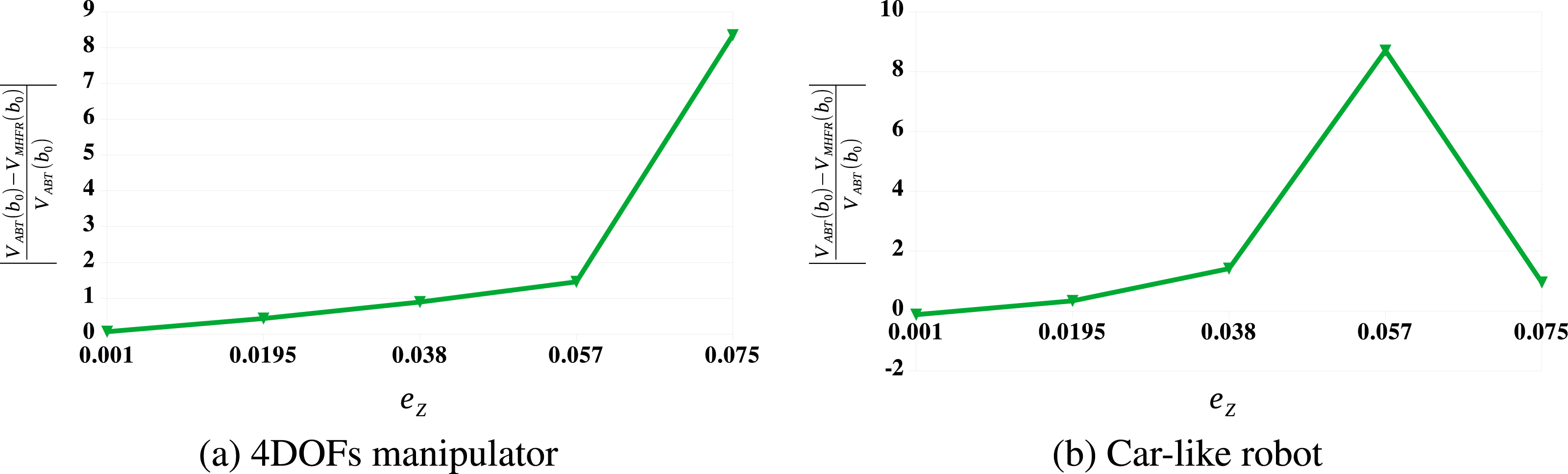

6.4. Testing SNM-planner

In this set of experiments, we want to test the performance of SNM-Planner in comparison with the two component planners ABT and MHFR. To this end, we tested SNM-Planner on four problem scenarios: The Maze scenario for the car-like robot shown in Figure 1(a) and the Factory scenario for the 4DOFs manipulator. The third scenario is the Kuka iiwa robot operating inside an office environment, as shown in Figure 1(b). Similarly to the Factory scenario, the robot has to reach a goal area while avoiding collisions with the obstacles. Finally, we tested SNM-Planner on the JacoCollab scenario described in Section 6.2.3 and shown in Figure 1(d). To further test the advantage of SNM in online POMDP planning compared to MoNG, we implemented a variant of SNM-Planner that uses MoNG as the heuristic instead of SNM. In particular, we replace line 5 in Algorithm 1 with a function approximateMoNG(b) that computes a local approximation of MoNG around the current belief b. Similarly to the method described in Section 4, we approximate MoNG for a set of state samples offline, and re-use the approximated MoNG values online.

To determine the best SNM and MonG thresholds, we first ran a set of preliminary tests using 10 values between 0.1 and 0.9. We found that for both measures, a value of 0.5 performed best across the scenarios. Thus, in all scenarios, we set the SNM and MonG threshold to 0.5. In Section 6.4.1 we provide a more in-depth analysis on how varying threshold values affect the performance of SNM-Planner. Additionally, for all scenarios, we use e _T = e _Z = 0.038. The planning time per step for the Maze and Factory scenario is 2s, while we use a planning time of 8s and 1s for the KukaOffice and JacoCollab scenarios, respectively.

The results in Table 3 and Table 4 indicate that SNM-Planner is able to approximately identify when it is beneficial to use a linearization-based solver and when a general solver should be used. In all four scenarios, SNM-Planner outperforms both the two component planners and MoNG-Planner. In the Maze scenario, the difference between SNM-Planner and the baselines is significant. The reason is, MHFR is well suited to compute a long-term strategy, as it constructs nominal trajectories from the current state estimate all the way to the goal, whereas the planning horizon of ABT is limited by the depth of the search tree. However, in the proximity of obstacles, the Gaussian belief assumption of MHFR are no long valid, and careful planning is required to avoid collisions with the obstacles. In general, ABT handles these situations better than MHFR. SNM-Planner combines the benefits of both planners and alleviates their shortcoming. Figure 8 shows state samples for which the SNM-values exceed the given threshold of 0.5. It is obvious that many of these samples are clustered around obstacles. In other words, when the support set of the current belief (i.e., the subset of the state space that is covered by the belief particles) lies in open areas, MHFR is used to drive the robot towards the goal, whereas in the proximity of obstacles, ABT is used to compute a strategy that avoids collisions with the obstacles. As we have seen in the previous section, MonG much less sensitive to obstacles in the environment compared to SNM. As a result, MoNG-Planner cannot replicate SNM-Planner’s strategic choice of the component planner, resulting in an overall worse performance.

Table 3.

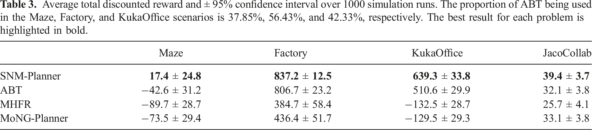
Average total discounted reward and ± 95% confidence interval over 1000 simulation runs. The proportion of ABT being used in the Maze, Factory, and KukaOffice scenarios is 37.85%, 56.43%, and 42.33%, respectively. The best result for each problem is highlighted in bold.

	Maze	Factory	KukaOffice	JacoCollab
SNM-Planner	17.4 ± 24.8	837.2 ± 12.5	639.3 ± 33.8	39.4 ± 3.7
ABT	−42.6 ± 31.2	806.7 ± 23.2	510.6 ± 29.9	32.1 ± 3.8
MHFR	−89.7 ± 28.7	384.7 ± 58.4	−132.5 ± 28.7	25.7 ± 4.1
MoNG-Planner	−73.5 ± 29.4	436.4 ± 51.7	−129.5 ± 29.3	33.1 ± 3.8

Table 4.

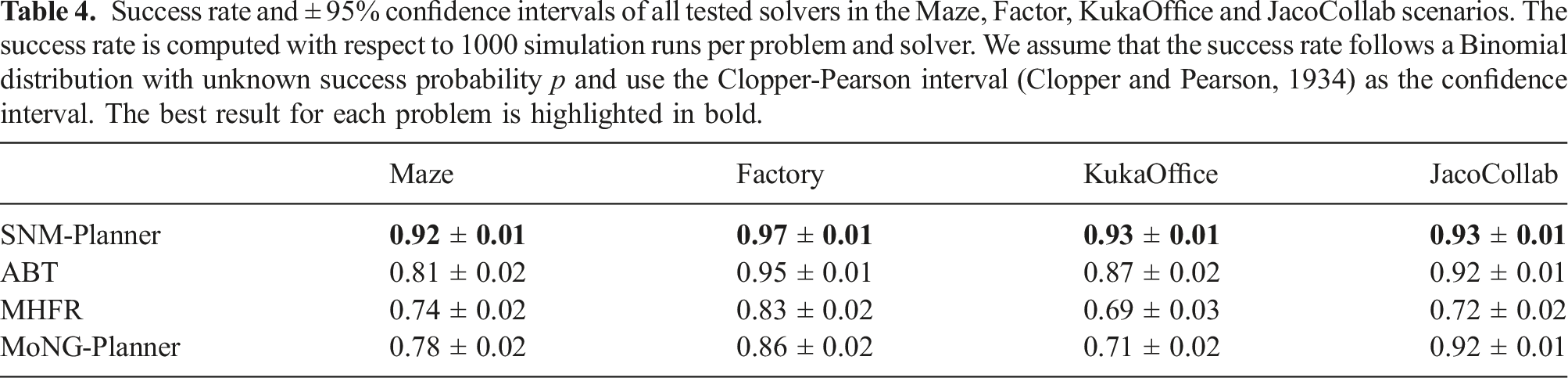
Success rate and ± 95% confidence intervals of all tested solvers in the Maze, Factor, KukaOffice and JacoCollab scenarios. The success rate is computed with respect to 1000 simulation runs per problem and solver. We assume that the success rate follows a Binomial distribution with unknown success probability p and use the Clopper-Pearson interval (Clopper and Pearson, 1934) as the confidence interval. The best result for each problem is highlighted in bold.

	Maze	Factory	KukaOffice	JacoCollab
SNM-Planner	0.92 ± 0.01	0.97 ± 0.01	0.93 ± 0.01	0.93 ± 0.01
ABT	0.81 ± 0.02	0.95 ± 0.01	0.87 ± 0.02	0.92 ± 0.01
MHFR	0.74 ± 0.02	0.83 ± 0.02	0.69 ± 0.03	0.72 ± 0.02
MoNG-Planner	0.78 ± 0.02	0.86 ± 0.02	0.71 ± 0.02	0.92 ± 0.01

Figure 8.

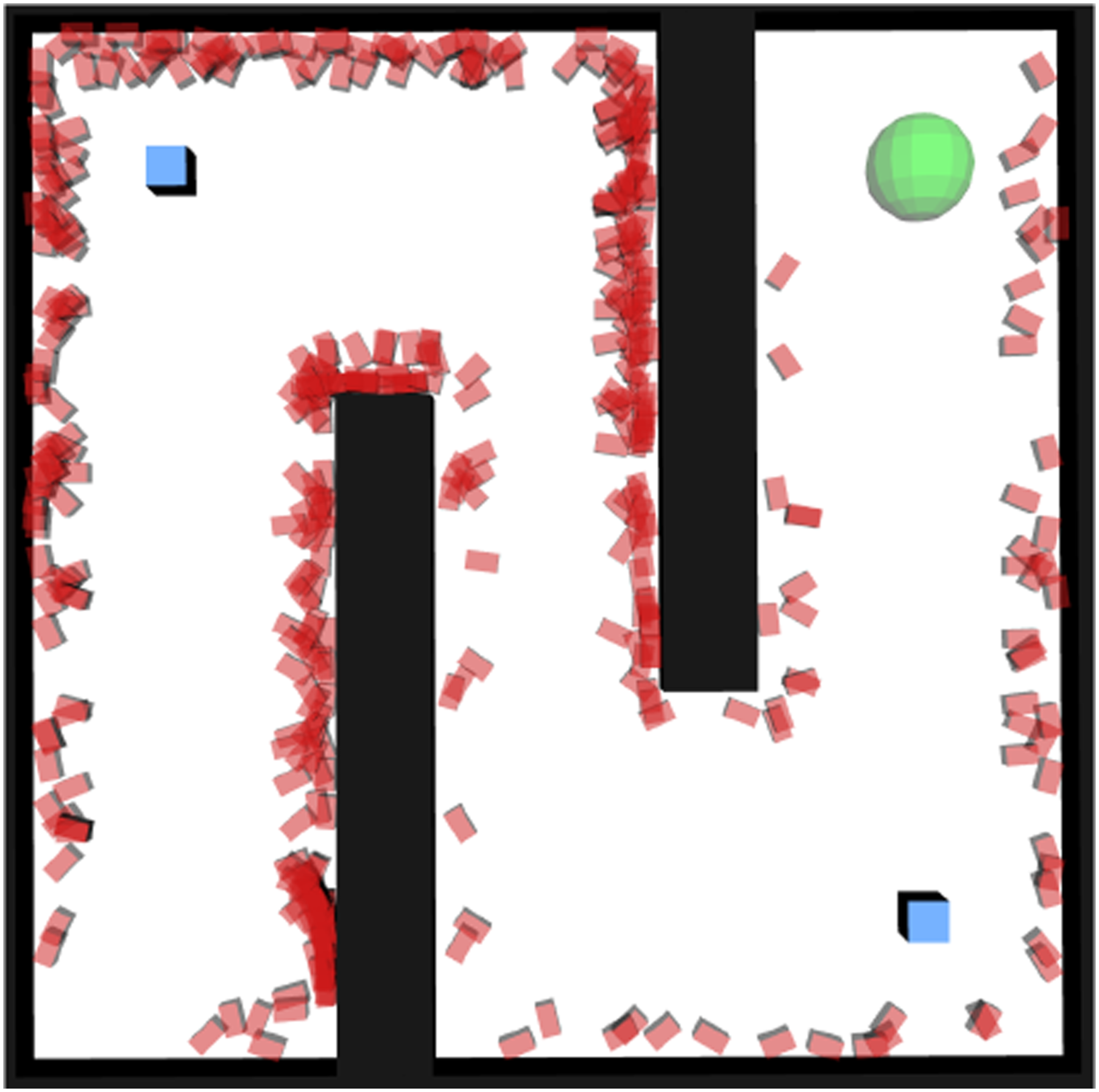
State samples in the Maze scenario for which the approximated SNM value exceeds the chosen threshold of 0.5.

A similar behavior was observed in the KukaOffice environment. During the early planning steps, when the robot operates in the open area, MHFR is well suited to drive the end-effector towards the goal area, but near the narrow passage at the back of the table, ABT in general computes better motion strategies. Again, SNM-Planner combines both strategies to compute better motion strategies than each of the component planners alone, while MoNG-Planner is unable to correctly identify situations in which MHFR or ABT should be used.

In the JacoCollab scenario, MHFR tends to compute strategies that move the robot to the goal as quickly as possible. However, those strategies are often too aggressive, resulting in collisions with the worker. On the other hand, for ABT, the robot tends to spend too much time in a safe region behind the worker, and only making slow progress towards the goal. SNM-Planner uses MHFR to compute a strategy that quickly leads to the goal, while it uses ABT when the robot is in the vicinity of the worker. This results in strategies that reach the goal quickly, while maintaining safety when the robot is near the worker, as reflected by the results in Table 3 and Table 4.

6.4.1. Sensitivity of SNM-planner and MonG-planner

In this experiment, we test how sensitive the performances of SNM-Planner and MonG-Planner are to the choice of the SNM and MonG thresholds, respectively. Recall that both planners use these thresholds to decide at each planning step which solver to use for the policy computation, based on a local approximation of the measures. For small thresholds the planners favor ABT, whereas for large thresholds MHFR is favored.

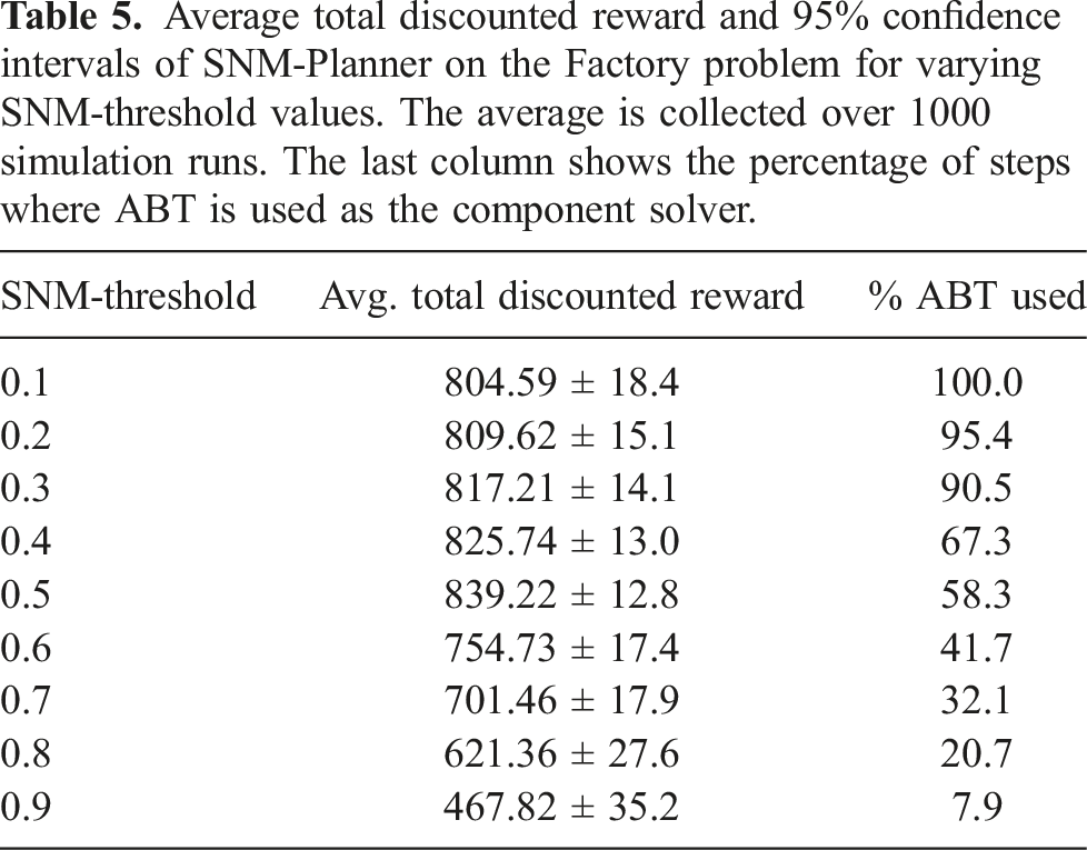
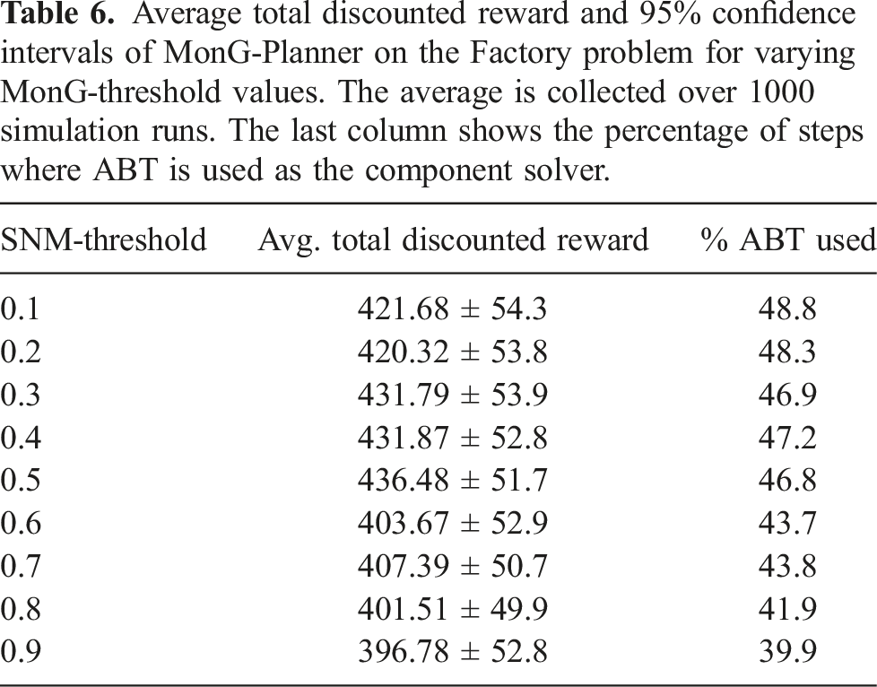
For this experiment, we test both SNM-Planner and MonG-Planner on the Factory problem (Figure 1(b)) with multiple values for the SNM and MonG thresholds, ranging from 0.1 to 0.9. For each threshold value, we estimate the average total expected discounted reward achieved by both planners using 1000 simulation runs. Here we set e _T = e _Z = 0.038.

Table 5 summarizes the results for SNM-Planner. It can be seen that the choice of the threshold can affect the performance of SNM-Planner, particularly for values that are on either side of the spectrum (very small values or very large values) where SNM-Planner favors only one of the component solvers. However, between the threshold values of 0.2 and 0.5 the results are fairly consistent, which indicates that there is a range of SNM-threshold values for which SNM-Planner performs well.

Table 5.

Average total discounted reward and 95% confidence intervals of SNM-Planner on the Factory problem for varying SNM-threshold values. The average is collected over 1000 simulation runs. The last column shows the percentage of steps where ABT is used as the component solver.

SNM-threshold	Avg. total discounted reward	% ABT used
0.1	804.59 ± 18.4	100.0
0.2	809.62 ± 15.1	95.4
0.3	817.21 ± 14.1	90.5
0.4	825.74 ± 13.0	67.3
0.5	839.22 ± 12.8	58.3
0.6	754.73 ± 17.4	41.7
0.7	701.46 ± 17.9	32.1
0.8	621.36 ± 27.6	20.7
0.9	467.82 ± 35.2	7.9

Table 6 shows the results for MonG-Planner. They indicate that the choice of the MonG-threshold has a minor effect on the performance of MonG-Planner. For all threshold values, MonG-Planner performs worse compared to SNM-Planner, which further indicates that SNM is more suitable in identifying situations where linearization is beneficial and where it should be avoided.

Table 6.

Average total discounted reward and 95% confidence intervals of MonG-Planner on the Factory problem for varying MonG-threshold values. The average is collected over 1000 simulation runs. The last column shows the percentage of steps where ABT is used as the component solver.

SNM-threshold	Avg. total discounted reward	% ABT used
0.1	421.68 ± 54.3	48.8
0.2	420.32 ± 53.8	48.3
0.3	431.79 ± 53.9	46.9
0.4	431.87 ± 52.8	47.2
0.5	436.48 ± 51.7	46.8
0.6	403.67 ± 52.9	43.7
0.7	407.39 ± 50.7	43.8
0.8	401.51 ± 49.9	41.9
0.9	396.78 ± 52.8	39.9

7. Summary and future work

This paper presents our preliminary work in identifying the suitability of linearization for motion planning under uncertainty. To this end, we present a general measure of non-linearity, called Statistical-distance-based Non-linearity Measure (SNM), which is based on the distance between the distributions that represent the system’s motion–sensing model and its linearized version. Comparison studies with one of state-of-the-art methods for non-linearity measure indicate that SNM is more suitable in taking into account obstacles in measuring the effectiveness of linearization.

We also propose a simple online planner that uses a local estimate of SNM to select whether to use a general POMDP solver or a linearization-based solver for robot motion planning under uncertainty. Experimental results indicate that our simple planner can appropriately decide where linearization should be used and generates motion strategies that are comparable or better than each of the component planner.

Future work abounds. For instance, the question for a better measure remains. The total variation distance relies on computing a maximization, which is often difficult to estimate. Statistical distance functions that rely on expectations exists and can be computed faster. How suitable are these functions as a non-linearity measure? Furthermore, our upper bound result is relatively loose and can only be applied as a sufficient condition to identify if linearization will perform well. It would be useful to find a tighter bound that remains general enough for the various linearization and distribution approximation methods in robotics.