Sage Journals: Discover world-class research

Abstract

When is heterogeneity in the composition of an autonomous robotic team beneficial and when is it detrimental? We investigate and answer this question in the context of a minimally viable model that examines the role of heterogeneous speeds in perimeter defense problems, where defenders share a total allocated speed budget. We consider two distinct problem settings and develop strategies based on dynamic programming and on local interaction rules. We present a theoretical analysis of both approaches and our results are extensively validated using simulations. Interestingly, our results demonstrate that the viability of heterogeneous teams depends on the amount of information available to the defenders. Moreover, our results suggest a universality property: across a wide range of problem parameters the optimal ratio of the speeds of the defenders remains nearly constant.

Keywords

Perimeter defense heterogeneous multi-robot team dynamic programming

1. Introduction

An increasingly important task where a robotic system can be employed is in defending an area against external agents, which pose varying levels of threat. Examples include defending airports against intruding and flight-grounding drones (Lykou et al., 2020), defending wildlife habitats against trespassing poachers (Casey, 2014), extinguishing and preventing the spread of devastating wildfires caused by human or natural activity (Cohen, 2007), as well as military applications (Zych, 2020).

In general, solutions to perimeter defense problems allude to finding strategies for a set of agents restricted to the perimeter of an area, entrusted with defending the area from intruders which are trying to breach the perimeter of the area (Shishika and Kumar, 2020).

Compared to a homogeneous team of robots, a team of robots with varying capabilities (heterogeneous team) comes with its unique set of advantages and challenges. Equipping different agents with different capabilities can lead to synergy effects where the heterogeneous system outperforms the alternative homogeneous system composed of identical agents. As a result, in the last decade, there has been significant interest in the robotics community to define, explore, and quantify heterogeneity in different robot applications (Mayya et al., 2022; Ramachandran et al. 2019, 2022; Ravichandar et al., 2020; Santos and Egerstedt, 2018; Twu et al., 2014).

This paper investigates the impact of heterogeneity in multi-robot teams for the perimeter defense problem.¹ We propose two optimal strategies, valid under different assumptions. The first strategy is based on dynamic programming (DP) (Cormen et al., 2001). It is optimal when the defenders are able to predict the location of the incoming attacks, but suffers from the curse of dimensionality and therefore relatively high associated computational costs. The second strategy is based on local interaction rules, and is optimal when the defenders have very limited information about the incoming attacks. This strategy can be efficiently computed in an online fashion, but does not implement any prior knowledge of the attack locations.

We prove the optimality of both strategies and analyze their time complexities, subject to a natural assumption (which will be discussed in detail in Section 5). The algorithms are extensively validated on simulations. Our numerical experiments are two-dimensional, but the majority of the theoretical results remain valid for any dimension. This includes three-dimensional perimeters in applications involving drones, and higher-dimensional perimeters arising as constraint sets in a state space of arbitrary dimension.

Our results show that heterogeneity is beneficial in the case where the defenders have access to information about the incoming attacks, and is detrimental when the defenders have very limited information about the attacks. Moreover, we show the universality property that the optimal ratio of the speeds of the defenders remains nearly constant for a two defender case setting.

For completeness, we also investigate the case of homogeneous defenders in order to establish the baseline properties of this model.

1.1. Related work

Perimeter defense problems are a variant of pursuit-evasion problems which have been studied extensively in literature. The seminal work of Issacs delineates differential-game approaches to arrive at equilibrium strategies for one pursuer one evader games (Isaacs, 1965). There has been considerable effort by researchers from various communities for solving various variants of pursuit-evasion games involving multiple pursuers and evaders (Fuchs et al., 2010; Von Moll et al., 2020; Yan et al., 2019). These papers contain works that view pursuit-evasion games either from the pursuers’ side, from the evaders’ side, or both. The curse of dimensionality poses a considerable challenge in solving problems involving multiple pursuers and evaders. The perimeter defense problem presented in this paper is a variant of the target guarding problem first introduced by Isaacs (Isaacs, 1965). In the target guarding problem setting an agent is tasked with guarding a region of interest against an adversarial agent. Investigations on perimeter defense problems are in their nascent stage. The review paper by Shishika and Kumar (Shishika and Kumar, 2020) delineates the recent works done on multi-robot perimeter defense problems (Guerrero-Bonilla et al., 2021; Lee et al., 2020; Shishika and Kumar, 2018; Shishika et al., 2019, 2020). Unlike the problems considered in these works, we consider a class of perimeter defense problems in which the number of attackers is much larger than the number of defenders. The authors of (Macharet et al., 2020; Velhal et al., 2022) consider the case of more attackers than defenders in similar (but distinct) contexts of homogeneous defenders. In particular, (Macharet et al., 2020) studies the problem of finite horizon attacks obeying an unknown probability distribution and partition the perimeter among the defenders. The authors of (Velhal et al., 2022) consider a decentralized method for allocating defenders to the incoming attacks. A one-defender analogue of the problem was previously considered in (Bajaj and Bopardikar, 2019; Chopra and Egerstedt, 2014; Smith et al., 2009) study a similar problem where attacks are assigned to defenders with differing skillsets (each attack can only be thwarted by a defender possessing a matching skill) with the goal of minimizing total defenders needed and total defender travel distance; however, their problem does not include constraints on defender speed, thus allowing any defender to reach any sequence of non-simultaneous attacks. Finally, Velhal et al. (2022) present and study a model which is very similar to our homogeneous defender perimeter defense problem; a full comparison and discussion is given in Section 4 and Appendix 5.

The remainder of the paper is organized as follows. Section 2 contains our notation together with the problem statement. Sections 4 and 5 detail our theoretical results in the infinite and unit-time horizon cases, respectively. Section 6 concludes with simulation results.

2. Problem statement

In this paper, bold letters are used to represent vectors and non-bold letters to represent scalars. Calligraphic letters are used to represent sets, and $| S |$ denotes the cardinality of a set $S$ .

For any positive integer $n \in Z^{+}$ , [n] denotes the set {1, 2, …, n}. For a domain $X$ with $x_{1}, x_{2} \in X$ , dist (x₁, x₂) denotes the length of the shortest path between x₁ and x₂ contained inside $X$ . As an example, in the case when $X$ denotes a circle of radius 1/2π

dist (x_{1}, x_{2}) = \frac{1}{2 π} \min (| θ_{1} - θ_{2} |, 2 π - | θ_{1} - θ_{2} |)

(1)

where θ₁, θ₂ are the polar angles of x₁ and x₂, respectively.

2.1. Perimeter defense against point attacks

For ease of reference, the notation of this section is summarized in Table 1. Our problem is perimeter defense against point attacks with mobile defenders of varying speeds. Specifically, we have a perimeter

X

in d-dimensional space, with a distance metric dist, defended by m mobile defenders with speeds v₁, …, v_m, so that defender i at

x \in X

at time t can make it to x′ at time t′ if and only if

dist (x, x^{'}) \leq (t^{'} - t) v_{i}

(2)

Table 1.

Notations.

Symbol	Description
$X$	Perimeter
m	Number of defenders
n	Number of attacks
x _i	Location of defender i
v _i	Speed of defender i, ordered decreasingly
z _j	Location of attack j
t _j	Time of attack j, ordered increasingly
h	Defender horizon
$Opt (v, {(z_{j}, t_{j})}_{j = 1}^{n})$	Minimum number of attacks the defenders can let through
$M (v, {(z_{j}, t_{j})}_{j = 1}^{n})$	Minimum number of defenders needed to defend against an attack sequence

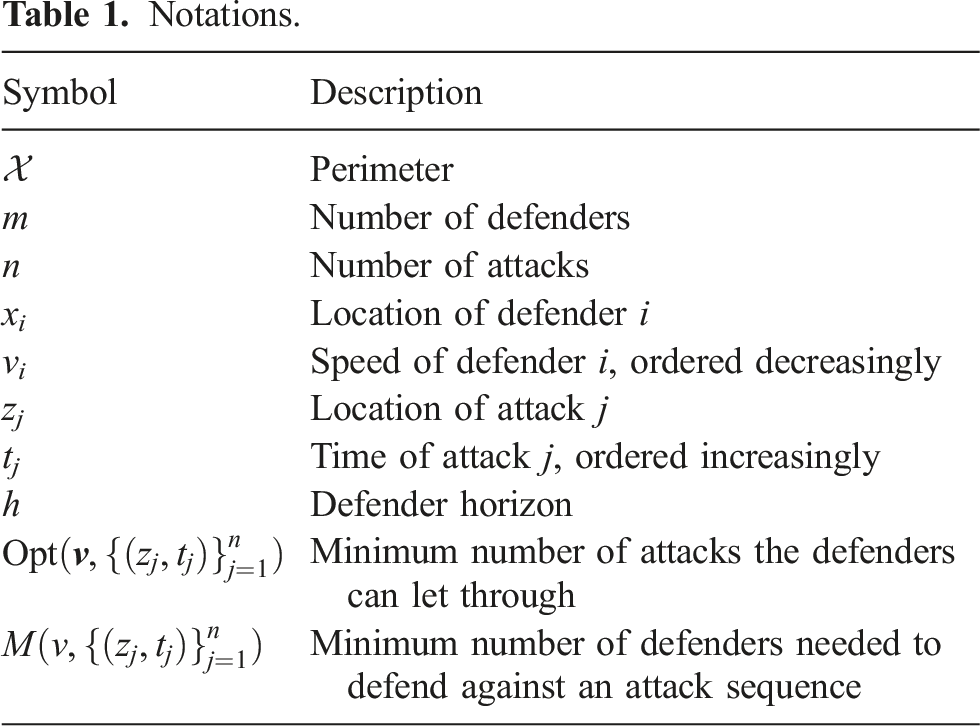
Without loss of generality we order the defenders from fastest to slowest, that is, v₁ ≥⋯ ≥ v_m, and we denote the speed vector as v = (v₁, …, v_m). Then n attacks $(z_{j}, t_{j}) \in X \times R_{\geq 0}$ , where z_j is the location on $X$ at which it happens, and t_j is the time; WLOG we order these by time, that is, t₁ ≤ ⋯ ≤ t_n (attacks at the same time can be ordered arbitrarily). Because attacks happen at fixed locations and times, they cannot react to the positions of the defenders. (Figure 1)

Figure 1.

Three defenders facing three attacks, with the unit-time reachable sets for each defender shown. Note that the third dimension is time; if the attack represents a physical object it is approaching from somewhere outside the circle, but we are only concerned with where and when it will hit the perimeter. In this example, the defenders are not allowed to leave the perimeter, so the size of the reachable set scales linearly with speed (until it covers the whole perimeter).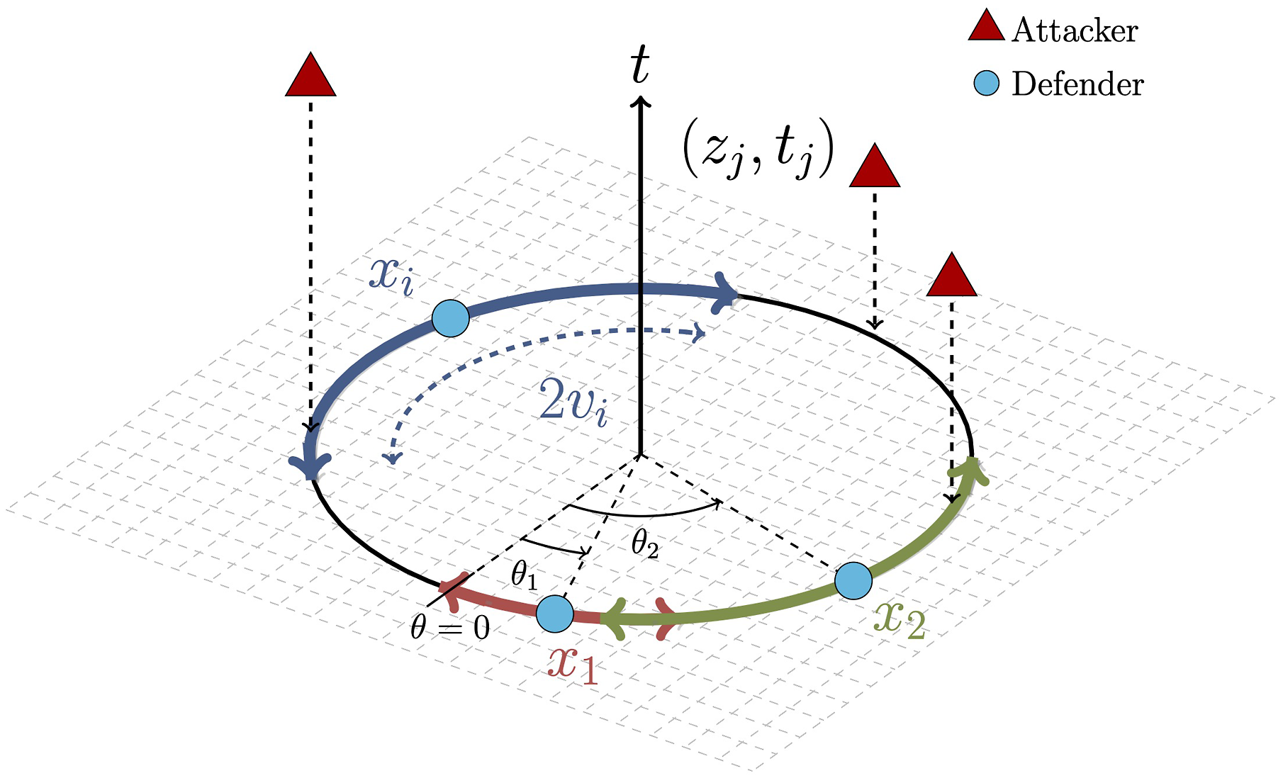

An attack (z_j, t_j) is thwarted if and only if a defender is present, that is, there is some defender i at z_j at time t_j; otherwise, we say that the attack breaches the perimeter. The goal is to design a policy for the defenders that minimizes the number of attacks that breach the defenses, and to study the effectiveness of different defender speed combinations against attacks.

Additionally, the team of defenders has a horizon h under which they can see attacks: specifically, at time t, any attack (z_j, t_j) is known to the defenders if and only if t_j ≤ t + h. We will study in particular the unit horizon h = 1 and the infinite horizon h = ∞ (all attacks are visible from the start).

Finally, the defenders are allowed to start at t = 0 at any combination of locations in $X$ ; they are even allowed to choose their starting locations based on the attack sequence (up to horizon h).

Given a speed vector v and sequence of attacks ${(z_{j}, t_{j})}_{j = 1}^{n}$ , we define $Opt (v, {(z_{j}, t_{j})}_{j = 1}^{n})$ as the minimum number of attacks from ${(z_{j}, t_{j})}_{j = 1}^{n}$ that defenders of speed v can let through (with all attacks known). We may compute $Opt (v, {(z_{j}, t_{j})}_{j = 1}^{n})$ for one sequence of attacks ${(z_{j}, t_{j})}_{j = 1}^{n}$ over many defender speed vectors v ; then we write Opt( v ) for convenience.

2.2. Different settings

Within the above problem description, there are several different variations, mostly to do with how the attacks are generated and the length of the horizon h. We roughly divide attack sequences into two settings:

1. Any sequence of attacks (z_j, t_j) is legitimate.

2. Attacks must come at unit-time intervals, that is, t_j = j for all j ∈ [n].

Note that in setting 2 we do not lose any generality by having the attacks happen at unit-time intervals, since we can rescale the time units (and adjust the speeds of the defenders accordingly). Since the index j is superfluous in setting 2 we refer to the sequence of attacks as z₁, z₂, …, z_n, indexed by t.

In setting 1, we study the case where all attacks are known to the defenders at the start; our primary problems are (i) find an algorithm for the defenders’ movements that minimizes the number of breaches, and (ii) study the behavior of optimal defense against uniformly random attacks (in both location and time) for different combinations of defenders. Since setting 1 is more general, the algorithms will also apply to setting 2.

In setting 2, we study the case where the attacks are (i) generated uniformly at random in location (time is fixed) and (ii) generated by an adversary which wants to guarantee a breach with as few attacks as possible. We also consider both the case where all the attacks are known to the defenders at the start (h = ∞) and the case where attack t only becomes known at time t − 1 (h = 1).

While in this work we mainly deal with the case where the number of defenders is fixed, and the question is how fast to make each defender (and in particular whether to make them all the same speed or not), we also investigate the alternative case of varying the number of (same-speed) defenders in Section 3, especially in regards to the tradeoff between fewer and faster defenders versus more and slower ones; we refer to this as the homogeneous setting. We show an efficient algorithm for determining the minimum number of (same-speed) defenders needed to thwart all attacks in a given attack sequence with infinite horizon, and empirically analyze how this minimum varies in expectation with the speed of the defenders. This shows that even the homogeneous setting has interesting and non-trivial properties that merit further study.

3. Homogeneous setting

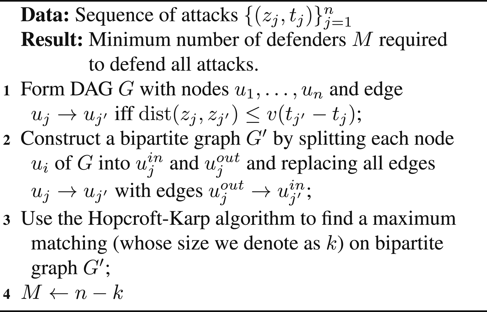
For a team of homogeneous defenders with speed v against a sequence of attacks ${(z_{j}, t_{j})}_{j = 1}^{n}$ , we show an algorithm for determining the minimum number $M (v, {(z_{j}, t_{j})}_{j = 1}^{n})$ of such defenders are needed to thwart all the attacks, which is based on reducing the problem to the well-known problem of maximum bipartite matching. For readability we denote the minimum number of defenders as $M : = M (v, {(z_{j}, t_{j})}_{j = 1}^{n})$ in this section and in Algorithm 1. The homogeneity of the defenders is key to this algorithm, which runs in time $O (\sqrt{n} | E |)$ where |E| is the number of edges in the DAG G; this is in turn proportional to n² in the worst case and hence the overall run time is O (n^5/2).

First, we build a directed acyclic graph (DAG) G on n nodes u₁, …, u_n, each node representing an attack; we assume that they are sorted by time t₁ ≤ t₂ ≤ … t_j (if not, we sort them in O (n log n) time). We put a directed edge u_j → u_j′ (where j′ > j) if and only if dist (z_j, z_j′) ≤ v (t_j′ − t_j), that is, if attack j′ can be reached by a defender which thwarts attack j.

Note that a (directed) path in G corresponds to a sequence of attacks that can be defended by a single defender. Thus, the goal is to decompose G into (the minimum) M directed paths which cover all vertices.

This path decomposition is done via a (well-known) reduction to maximum bipartite matching: we split each node u_j into $u_{j}^{i n}$ and $u_{j}^{o u t}$ , where a directed edge $u_{j}^{i n} \to u_{j}^{o u t}$ exists, and all edges u_j → u_j′ are replaced with edges $u_{j}^{o u t} \to u_{j^{'}}^{i n}$ . This does not change the minimum M.

Taking ${u_{j}^{o u t}}$ and ${u_{j}^{i n}}$ as the two parts of a bipartite graph (and ignoring the $u_{j}^{i n} \to u_{j}^{o u t}$ edges), any matching on this graph can be used to reconstruct a set of nonoverlapping paths that cover all the vertices of G by putting back the $u_{j}^{i n} \to u_{j}^{o u t}$ edges; since each $u_{j}^{i n}$ has exactly one edge coming out of it (to $u_{j}^{o u t}$ ) and each $u_{j}^{o u t}$ has at most one edge coming out of it (if it is matched it has one, otherwise not) one can start at any unmatched $u_{j}^{i n}$ and uniquely walk forward until reaching some unmatched $u_{j^{'}}^{o u t}$ , producing one directed path.

Since there is one such path starting at each unmatched $u_{j}^{i n}$ (and ending at each unmatched $u_{j^{'}}^{o u t}$ ), a matching of size k produces a set of M = n − k directed paths covering the vertices of G (and conversely any set of M directed paths can be used to find a size-(n − M) sized matching). Thus, finding the maximum k gives the minimum number of defenders $m = M (v, {(z_{j}, t_{j})}_{j = 1}^{n})$ .

Thus, we can use any well-known maximum bipartite matching algorithm (e.g., Hopcroft-Karp) to compute the number of defenders needed.

Remark 1

Note that a complete matching (which would imply that 0 defenders could thwart all the attacks!) is by definition impossible because G is acyclic.

The algorithm is summarized in Algorithm 1 for ease of reference.

Algorithm 1: Homogeneous case

Taking the matching produced by Algorithm 1 and adding the edge $u_{j}^{i n} \to u_{j}^{o u t}$ for all j yields the assigned defender trajectories.

3.1. Complexity

There are two parts to this problem:

1. Building DAG G and its bipartite counterpart G′.

2. Computing the maximum matching.

Ignoring d, which we assume to be small, (1) takes O (n²) time, and (2) with Hopcroft-Karp takes $O (\sqrt{n} | E |)$ where E is the number of edges, which in the worst case means O (n^5/2).

3.2. Extension to cost minimization

As mentioned in Section 1, a very similar problem to the homogenous defender problem discussed in this section was studied in Velhal et al. (2022).² Under the same threat model (attacks occur at certain times and places, and a team of homogeneous defenders must intercept all of them), they extended the question to include the minimization of fuel cost (as measured in total travel distance of the defenders) while minimizing the number of defenders. They first consider a version with a fixed number of defenders; in this case the only objective is to defend all attacks while minimizing fuel cost. They formulate this as an instance of the Linear Sum Assignment Problem (LSAP), which can be solved by successive applications of Djikstra’s Algorithm in O (n³) total time (if there are insufficiently many defenders to defend the perimeter, the solution instead gives the smallest possible number of attacks which must be left undefended). They then use repeated applications of the LSAP to find the minimum number of defenders needed to protect the perimeter, and then minimize the fuel cost. Although in their work they claim that a single call to the LSAP suffices to determine the minimum number of defenders, we believe that multiple calls (naively up to even O (log n)) are necessary; see Appendix 5 for details.

In contrast, our problem seeks only to minimize the number of defenders, since our focus in this section is to characterize the tradeoff between the speed of the defenders and the number needed to protect the perimeter. Thus, in contrast to their solution, which relies on solving a complexity-O (n³) problem, we can achieve this in O (n^2.5) in the worst case via reduction to maximum bipartite matching.

Nevertheless, inspired by their results, we note that our algorithm can be extended to cover the cost minimization problem as well (with an arbitrary cost function for traveling between locations, where the objective is to minimize the sum of the costs of travel): Suppose the cost of moving from attack j to j′ is given by c_j,j′ ≥ 0 (if moving from j to j′ is feasible). Then, after constructing the DAG G with edges E and its bipartite counterpart G′ as in Algorithm 1, we apply a weight to edge 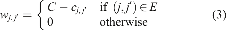$u_{j}^{o u t} \to u_{j^{'}}^{i n}$ of

w_{j, j^{'}} = {\begin{cases} C - c_{j, j^{'}} & if (j, j^{'}) \in E \\ 0 & otherwise \end{cases}

(3)

where C = 1 + ∑_j,j′c_j,j′. Then, finding the maximum-weight bipartite matching on G′ with weights w_j,j′ yields the min-cost assignment for the minimum number of defenders. This is because C is sufficiently large that matchings with more edges will always have more weight than matchings with fewer edges (thus using fewer defenders is always better); and among the maximum-size matchings, maximizing the sum of the weights w_j,j′ is equivalent to first minimizing the number of defenders, and then (given the minimum number of defenders) minimizing the sum of the costs c_j,j′ of the edges in the matching.

Thus, our technique reduces this problem to an instance of the Assignment Problem with weights w_j,j′, which can be solved in O (n³) time by the Hungarian Algorithm. Solving this problem minimizes both number of defenders and cost simultaneously.

4. Infinite horizon theoretical results

We now turn to the question of heterogeneous teams.

4.1. Dynamic programming with infinite horizon

We now give an algorithm which, given defender speeds v = (v₁, …, v_m) and attacks ${(z_{j}, t_{j})}_{j = 1}^{n}$ returns two quantities: (i) $Opt (v, {(z_{j}, t_{j})}_{j = 1}^{n})$ (the minimum number of attacks that can be let through); and (ii) the list (of lists) ℓ = (ℓ₁, …, ℓ_m), where ℓ_i is the (sub)sequence of attacks which defender i thwarts. We refer to ℓ as a defense plan.

Recall that by default the attacks are sorted in order of arrival time (or the user should sort them before applying the algorithm).

The pseudocode is given in Algorithm 2, in which we use the following notation: j = (j₁, …, j_m) ∈ {0,1,…,n}^m denotes a vector of attacks assigned to each defender (with j_i = 0 indicating no attack assigned to defender i, and we allow the j_i’s to be non-distinct even though it is redundant);

j_{- i} (j^{'}) = (j_{1}, \dots, j_{i - 1}, j^{'}, j_{i + 1}, \dots, j_{m})

(4)

that is, j with the ith entry replaced by j′;

1_{i} (j^{'}, j^{″}) : = {\begin{cases} 1 & dist (z_{j^{'}}, z_{j^{″}}) \leq (t_{j^{″}} - t_{j^{'}}) v_{i} \\ 0 & otherwise \end{cases}

(5)

is the indicator that defender j is capable of thwarting attack j″ after thwarting j′ (and 1 _i (0, j″) = 1 since defenders can start anywhere); [·] + [·] denotes concatenation (of lists); and arg min (arg max) denote the sets of values minimizing (maximizing) the arguments.

Algorithm 2 then works by recursively computing the function $V (j) : {0, 1, \dots, n}^{m} \to N$ , which denotes the following: suppose that defender i (with speed v_i) is required to thwart attack j_i and then no others after that (but defender i can thwart attacks arriving before $t_{j_{i}}$ , and if j_i = 0, then defender i is not allowed to thwart any attack); V( j ) is the minimum number of defenders that can be let through under these constraints. Then the following hold:

• V (0, …, 0) = n (the base case from which we recursively compute V), which holds since j = (0, …, 0) denotes the situation where no attacks are assigned to any defender so all the attacks breach;

• $Opt (v, {(z_{j}, t_{j})}_{j = 1}^{n}) = \min_{j} V (j)$ (this allows us to extract the correct value by keeping track of this minimum); while Algorithm 2 iterates, it also keeps track of the assignment j ^min which currently minimizes V( j ) which also allows it to reconstruct the optimal defender paths.

The for-loop in Algorithm 2 computes V( j ) recursively by iterating over assignments j in lexicographic order (skipping the base case j = (0, …, 0)). Note that all values sharing the use of the letter “j” refer to attack indices. Each iteration in Algorithm 2 refers to an assignment of attackers to defenders denoted j = (j₁, …, j_m), where j_i is the index of the attack assigned to defender i, and j ^min is the assignment that (currently) minimizes the number of attacks let through.

The proof of the following result is given in Appendix 1:

Theorem 1

Algorithm 2 outputs the correct value of $Opt (v, {(z_{j}, t_{j})}_{j = 1}^{n})$ and ℓ .

See Figure 2 for an example and Appendix 1 for the details.

Figure 2.

Computing V (6, 2, 4) (defender 1 has to thwart attack 6, etc.,) recursively; each defender is allowed to thwart attacks prior to these, but not afterward. Since 6 is the maximum value, we consider the last attack that defender 1 can handle before 6: based on its speed, it can be 0 (defend nothing before 6), 1, or 3. Thus V (6, 2, 4) = min (V (0, 2, 4), V (1, 2, 4), V (3, 2, 4)) − 1.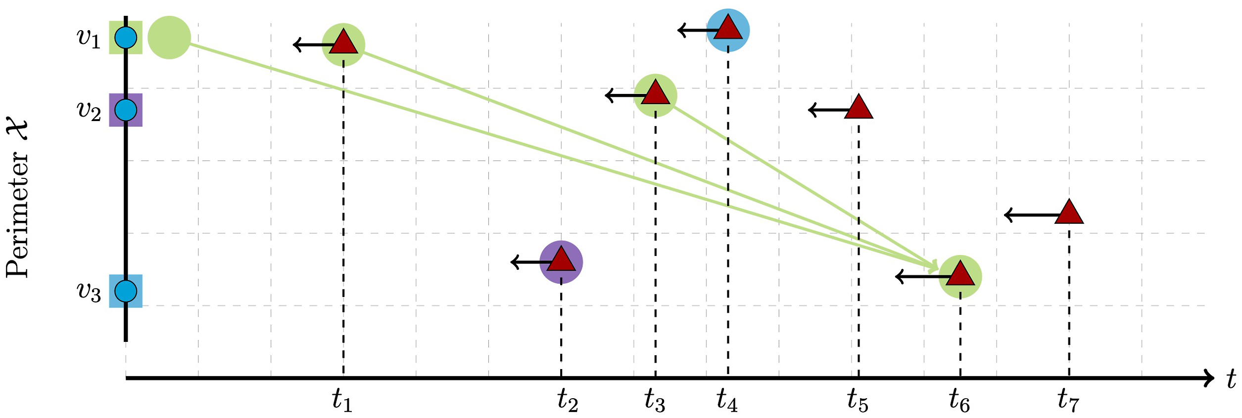

Algorithm 2: Dynamic programming for infinite horizon defenders.

Remark 2

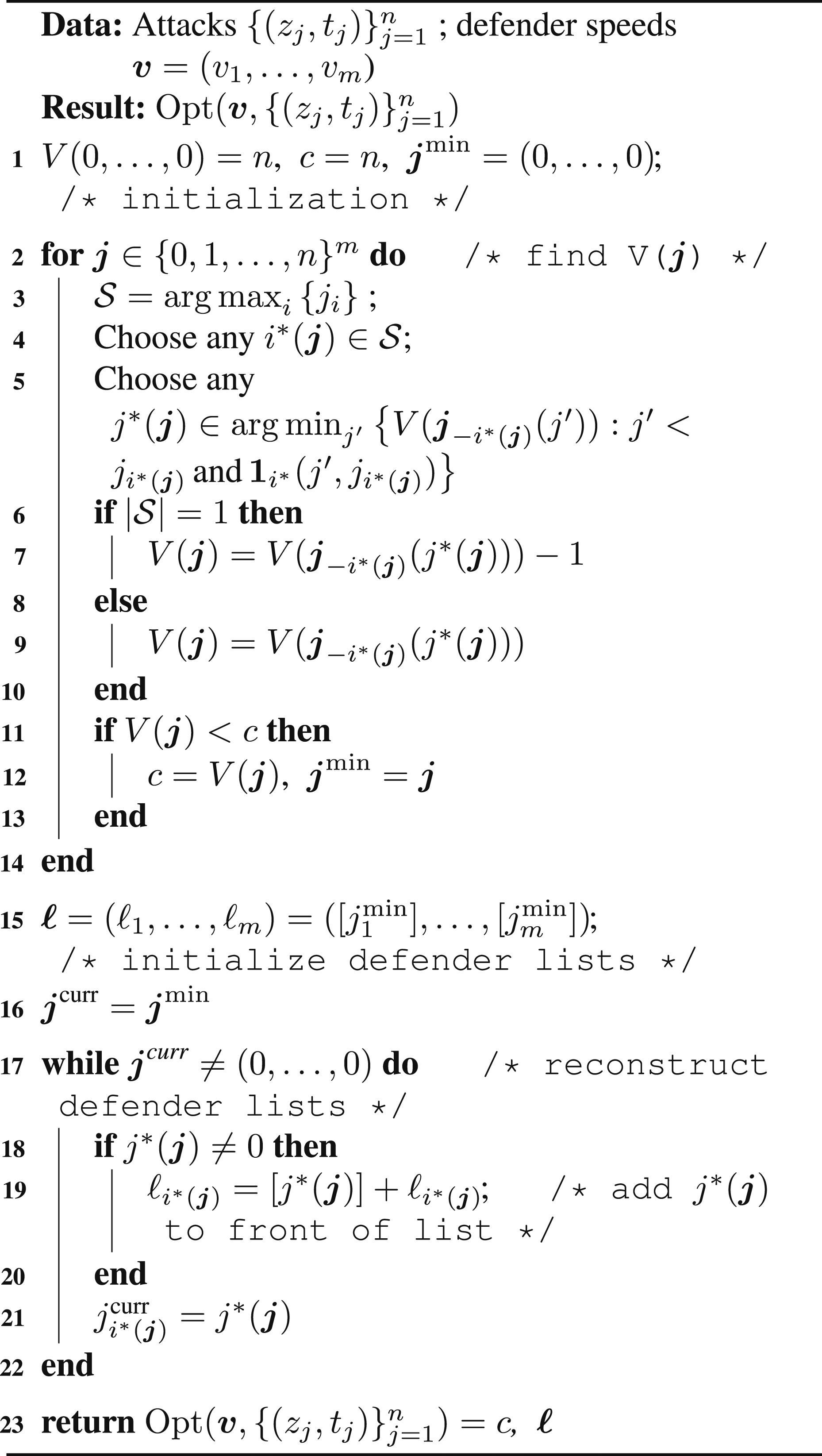
Algorithm 2 relies on the subtle point that i*( j ) ∈ arg max_i j_i because if not, then we do not know whether to subtract 1 when we do the update; by setting i*( j ) ∈ arg max_i j_i, we remove the question of whether a defender i′ assigned to a later j_i′ can also thwart attack $j_{i^{*}}$ .

Remark 3

Algorithm 2 assumes that the defenders can start at whatever locations they want, but can be modified for fixed defender starting locations (or a set of possible starting locations) by redefining 1 _i(0, j) to indicate whether they can reach attack j from their starting locations. It can also be modified for the important case where attacks cause varying amounts of damage, with attack j doing w_j damage (should it not be intercepted); see for instance the Iron Dome missile defense system, which prioritizes attacks based on potential damage estimates (Zych, 2020). To make this modification, replace −1 with $- w_{j_{i^{*} (j)}}$ in line 7 and V(0, …, 0) = c = n with V(0, …, 0) = c = ∑_jw_j.

Given m defenders and n attackers, the number of computations needed to run Algorithm 2 is O ((n + 1)^m+1) (we need to run through (n + 1)^m values of j , and each update takes up to n time for the comparisons). While this is polynomial for any fixed value of m, it is exponential in general relative to the size of the problem (and gets too expensive in practice quickly as m is increased). This raises the question of the complexity of computing $Opt (v, {(z_{j}, t_{j})}_{j = 1}^{n})$ ; while a valid solution can be easily verified it remains open whether it is NP-Hard, or if other improvements to the algorithm can be made.

4.2. Monotonicity-based computational acceleration

In order to investigate team heterogeneity, we compute $Opt (v, {(z_{j}, t_{j})}_{j = 1}^{n})$ for all v whose elements v_i are at g evenly spaced locations in a range (v_min, v_max].³ We refer to g as the number of grains. If we were to run Algorithm 2 for all combinations v of speeds, the complexity becomes O ((n + 1)^m+1g^m), which gets extremely large very quickly.

However, as each attack sequence is evaluated on all v , we can take advantage of the monotonicity of Opt over v to reduce the amount of computation needed.

In particular, for any sequence ${(z_{j}, t_{j})}_{j = 1}^{n}$ ,

v \leq v^{'} \Rightarrow Opt (v) \geq Opt (v^{'})

(6)

since faster defenders can always emulate slower ones and thus achieve (at least) as good a result on any attack sequence. This means that

Opt (v) = Opt (v^{'}) = k for some v \leq v^{'}

(7)

\begin{array}{l} \Rightarrow & Opt (v^{″}) = k for all v \leq v^{″} \leq v^{'} \end{array}

(8)

Thus we know Opt ( v ″) = k for a range of v ″, without having to run Algorithm 2. Taking the set of values $v \in {(v_{\min}, v_{\max}]}^{m}$ (of given grains), for any ${(z_{j}, t_{j})}_{j = 1}^{n}$ we can evaluate $Opt (v, {(z_{j}, t_{j})}_{j = 1}^{n})$ in a strategic order to minimize the number of times we need to run Algorithm 2.

We now describe this order in greater detail. While we have not made any rigorous attempt to optimize the ordering, the order we use was effective enough to reduce the computation of the simulations described in the main work (see Figures 3 and 5, left-hand column for uniformly random attack times and right-hand for fixed attack times) by an average of between 93% and 99% depending on the parameters; the savings are much more pronounced for the fixed attack times case, as the Opt function is generally flatter (and hence produces more cases where the upper bound matches the lower bound and the DP computation can be skipped).

Figure 3.

The quantity w as a function of v₁ and v₂, with the regions defined by Theorem 2 removed.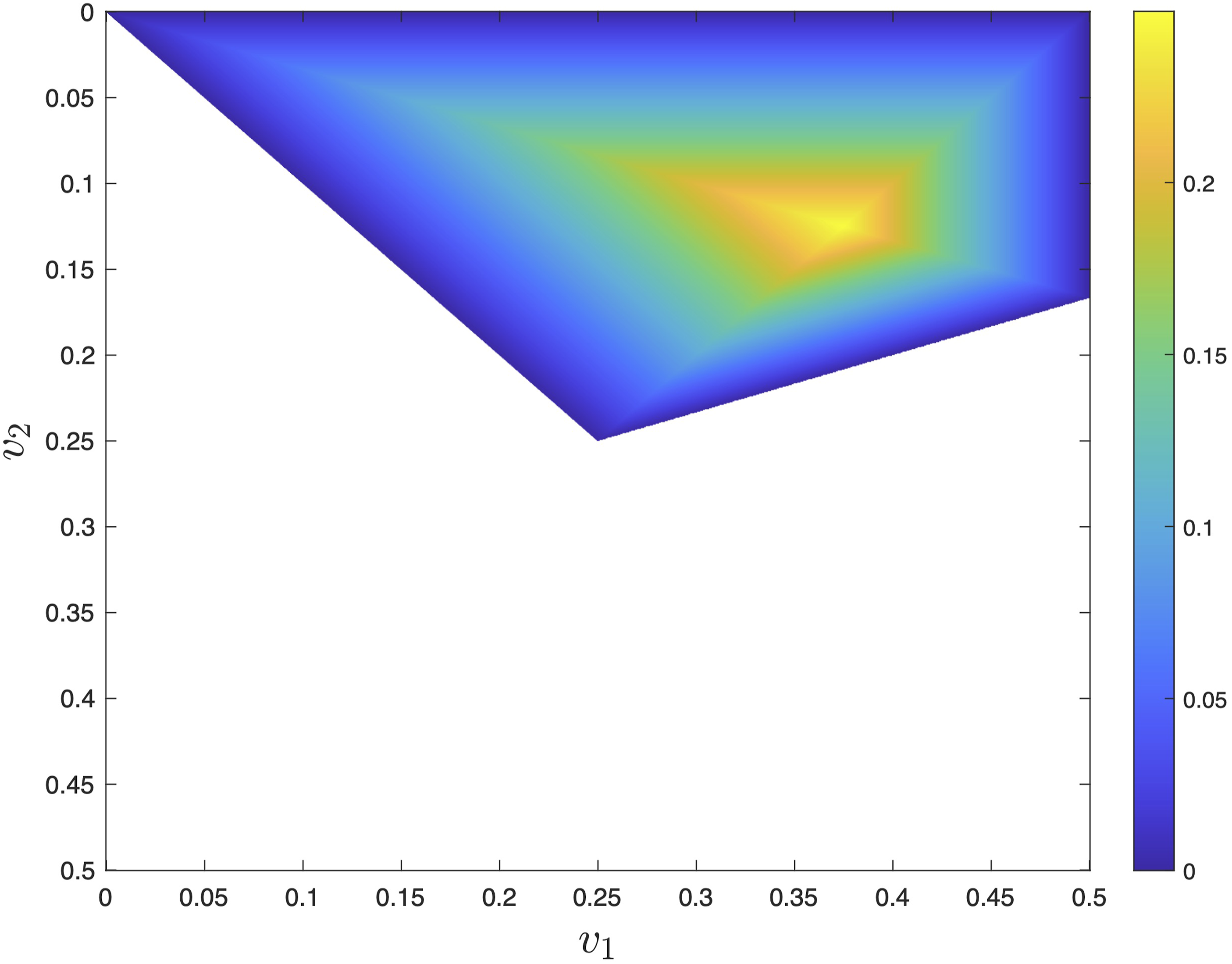

First, it is noted that permuting v does not affect Opt( v ); hence whenever Opt (v₁, v₂) is computed, we get the same value for Opt (v₂, v₁) (recall that in these simulations we drop the WLOG assumption that v₁ ≥ v₂). For simplicity we will talk about the indices of the speed values we compute for: the goal is to compute Opt( v ) for all v with entries from a range of g values, which we will denote as a vector w = (w₁, …, w_g) where w₁ < w₂ < … < w_g without loss of generality. Then we define a function $V : {[g]}^{m} \to R$ , where

V (j_{1}, \dots, j_{m}) = Opt (w_{j_{1}}, \dots, w_{j_{m}})

(9)

This just means that the ith defender has speed $v_{i} = w_{j_{i}}$ . Since w is monotonically increasing (in its entries) and Opt is monotonically decreasing, V is monotonically decreasing as well. For this section, as in the simulations, m = 2 so we can visualize [g]^m as a grid (as in Figure 5 in the main paper).

The basic idea is to compute in order of decreasing powers of 2, which we refer to as levels: for instance, when g = 256 we compute first for multiples of 256, then multiples of 128, then 64 and so forth. In this way, at each level we can use the results from the level above to check the monotonicity condition and potentially save significant computation.

The algorithm then does the following:

1. Compute V (j₁, j₂) for the four corners of the grid.

2. Compute V (j₁, j₂) on the edges and main diagonal of the grid, in decreasing powers of 2. This establishes a border so that every subsequent step has an upper bound and a lower bound to compare.

3. Compute V (j₁, j₂) by decreasing levels (at each level, doing it in lexicographic increasing order as normal, skipping any entries already computed previously).

We also for simplicity only considered the upper and lower bounds generated by previous entries on the same row or column of the grid (two upper bounds, one for the row and one for the column, to two lower bounds, also one for the row and one for the column).

5. Unit-horizon theoretical results

This section considers defenders with a unit horizon of incoming attacks. The general setup is

• We consider two defenders with speeds v₁ ≥ v₂.

• We consider a perimeter $X$ homeomorphic to $S^{1}$ (a circle⁴), with distances determined by arc length and total length normalized to 1; we represent $X = [- 1 / 2, 1 / 2]$ (but −1/2 and 1/2 are the same point). To denote this situation, we define the distance function

dist (y_{1}, y_{2}) = \min {| y_{1} - y_{2} |, 1 - | y_{1} - y_{2} |}

(10)

(a rescaled version of equation (1)). The maximum possible value of dist (y₁, y₂) is 1/2, and we assume they start at maximum distance from each other, that is, at antipodal points.

• The n attackers are generated according to Setting 2 from Section 2: attacker t appears at time t, uniformly (and independently) over $X$ .

• The defenders have a unit horizon in time: at any given time they only see the next incoming attack, though they also know n and the current time t.

Therefore the defenders’ policy can be thought of as a sequence of decisions taken at unit-time intervals (i.e., when the next attack is revealed), which is naturally formulated as a Markov Decision Process (MDP) (Puterman, 2014) with n steps, with the reward being the number of thwarted attacks.

To simplify the MDP we can remove one state variable since, by symmetry, we can rotate $X$ (or relabel it) so that at the beginning of any time step, defender 1 is at location 0. We can also reflect it so that defender 2 is on the positive half. Thus the state at time t (just before the location of the next attack is revealed) can be denoted by a single parameter a(t), indicating the distance between the two defenders. Then the next attack’s location x (t + 1) is revealed, in the coordinate system relative to the defenders’ positions.

5.1. Policy and reward

A unit-horizon policy is a function $f : [0, 1 / 2] \times [- 1 / 2, 1 / 2] \times Z_{> 0} \to [0, 1 / 2]$ . The inputs are a(t), x(t) and the number of remaining attacks N, and the output is f (a(t), x(t), N) = a (t + 1). As described above, a (t + 1) is the distance between the two defenders at time t + 1. f must satisfy the condition

f (a (t), x (t), N) \in [a (t) - v_{2} - v_{1}, a (t) + v_{2} + v_{1}]

(11)

The policy then produces a reward

r (t) : = r (a (t), x (t), f (a (t), x (t), N)) \in {0, 1}

(12)

the reward, based on whether the given movement makes it possible for the attack to be thwarted (r(t) = 1 if so, = 0 if not). r(t) is given as follows:

r (t) = {\begin{cases} 1 & if dist (0, x (t)) \leq v_{1} and \\ f (a (t), x (t), N) \in [dist (x (t), a (t)) - v_{2}, \\ dist (x (t), a (t)) + v_{2}] \\ 1 & if dist (a (t), x (t)) \leq v_{2} and \\ f (a (t), x (t), N) \in [x (t) - v_{1}, x (t) + v_{1}] \\ 0 & otherwise \end{cases}

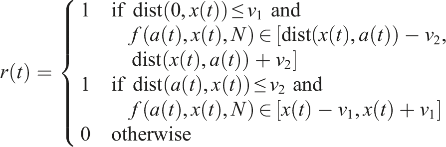
The reason for this is that by symmetry (of the perimeter and of the attacks), the ability of the defenders to stop future attacks depends only on their distance a (t + 1) = f (a(t), x(t), N). Thus, if the defenders can stop the current attack and end at distance a (t + 1) = f (a(t), x(t), N) for the next step, it is always best to do so (as opposed to ending at the same distance without stopping the attack).

So r(t) = 1 under policy f if and only if this is possible, which can be split into two cases: (i) defender 1 makes the capture; (ii) defender 2 makes the capture. If either of these are feasible, r(t) = 1; if neither are, r(t) = 0.

Remark 4

If dist(a(t), x(t)) > v₂ and dist(0, x(t)) > v₁, this means that neither defender can reach the next attack and hence r(t) = 0 no matter what.

5.2. Optimal defender policy

Fix a defender policy f. For a given total number N of incoming attacks and an initial distance a between the two defenders, we define the expected reward J (a; N) of the defenders as the expected total number of thwarted attacks, that is,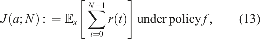

J (a; N) : = E_{x} [\sum_{t = 0}^{N - 1} r (t)] under policy f,

(13)

where the expectation is over the attack locations x(t). With this definition, we are interested in determining the policy f that leads to the highest expected reward.

We first show necessary and sufficient conditions for perfect defense, that is, when no (fixed-time) attack sequence can force a breach.

Theorem 2

(The perfect defense theorem). For any pair of defenders with speeds v₁, v₂ where v₂ ≤ v₁, there exists a sequence of attacks that breaches if and only if v₁ < 1/2 and v₁ + 3v₂ < 1; whereas, if v₁ ≥ 1/2 or v₁ + 3v₂ ≥ 1, the defenders can defend indefinitely even with a one-step horizon. Furthermore, if any sequence of attacks guarantees a breach, there also exists a sequence (not necessarily a subsequence) of at most 6 attacks that does so.

Proof

The proof is given in Appendix 1.

Next, we conjecture that it is always optimal to thwart a reachable attack; furthermore, we prove that under certain conditions (specifically, if the number of future attacks is sufficiently small relative to a parameter dependent on the defender speeds) then thwarting it is always optimal. The following result shows that, for a wide range of values for v₁, v₂ and N, the optimal strategy should (i) always thwart the currently known if possible.

Proposition 1

Let

w = \min (1 - 2 v_{1}, 1 - v_{1} - 3 v_{2}, 2 v_{2}, v_{1} - v_{2})

and let the current separation between the defenders be a ≥ 2v₂; then if there are N ≤1/w attacks left after the current attack, thwarting the current attack (if possible) is always optimal.

Proof

The proof is given in Appendix 2.

The value w is maximized when v₁ = 3/8 and v₂ = 1/8, yielding w = 1/4. We also show w as a function of v₁ and v₂ in Figure 3, with the regions defined by Theorem 2 removed, since these guarantee perfect defense and hence that all attackers can and should be captured.

Note also that the above holds as well if the number of future attacks is random (unknown to the defenders) with $E [N]$ replacing N. We note that the bound above is not the best achievable by this method; we can sharpen it by a more careful consideration of the properties of the optimal policy, as discussed in more detail in Appendix 2.

We next prove that the optimal policy subsequently should (ii) always maximize a(t) subject to the first constraint. That is,

Proposition 2

f* maximizes J(a; N) if (ii) a(t + 1) is maximized for all inputs, over all policies that satisfy (i) (i.e., capture when possible).

Proof

The proof is given in Appendix 3.

6. Simulation results

6.1. Simulations for homogeneous defenders

The goal of the simulations is to explore the relationship between speed and number of defenders (if we halve the speed of the defenders, how many more do we need to keep the same level of effectiveness?)

Our experiments follow the pattern:

1. Generate attacks ${(z_{j}, t_{j})}_{j = 1}^{n}$ randomly, either with fixed attack times t_j = j or uniformly random attack times in [0, t_max].

2. Compute the minimum number of defenders $M (v, {(z_{j}, t_{j})}_{j = 1}^{n})$ to defend against the sequence for $v \in (v_{\min}, v_{\max}]$ or $v \in {(v_{\min}, v_{\max}]}^{m}$ , at g intervals.

3. Repeat the above for T trials and average the resulting values for each value of v or v .

We compute $M (v, {(z_{j}, t_{j})}_{j = 1}^{n})$ for all v whose v_i are at g evenly spaced locations in the range (v_min, v_max] of speeds. We refer to g as the number of grains.

The full list of parameters is given in Table 2.

Table 2.

Parameters of the experiments.

Symbol	Description
m	Number of defenders (m = 2 unless specified otherwise)
n	Number of attacks
T	Number of trials
t _max	Size of attack window (not needed for heterogeneous setting (ii))
(v_min, v_max]	Range of defender speeds (inclusive of v_max but not v_min)
g	Number of speed values measured (grains) within (v_min, v_max]

For ease of notation, we denote

E [M (v)] : = E [M (v, {(z_{j}, t_{j})}_{j = 1}^{n})]

(14)

The expectation is over the attacks, that is, random (z_j, t_j). All experiments are for uniformly random attack times on a circular (1-dimensional) perimeter of circumference 1.

Our simulations suggest a strong relationship between the speed v of the homogeneous defenders and the expected number $E [M (v)]$ of defenders required to thwart all attacks: plotting these in a log-log plot reveals an almost linear relationship between log v and $\log (E [M (v)] - 1)$ , as shown in Figure 4.5

Figure 4.

Log-log plots of v versus (empirical) 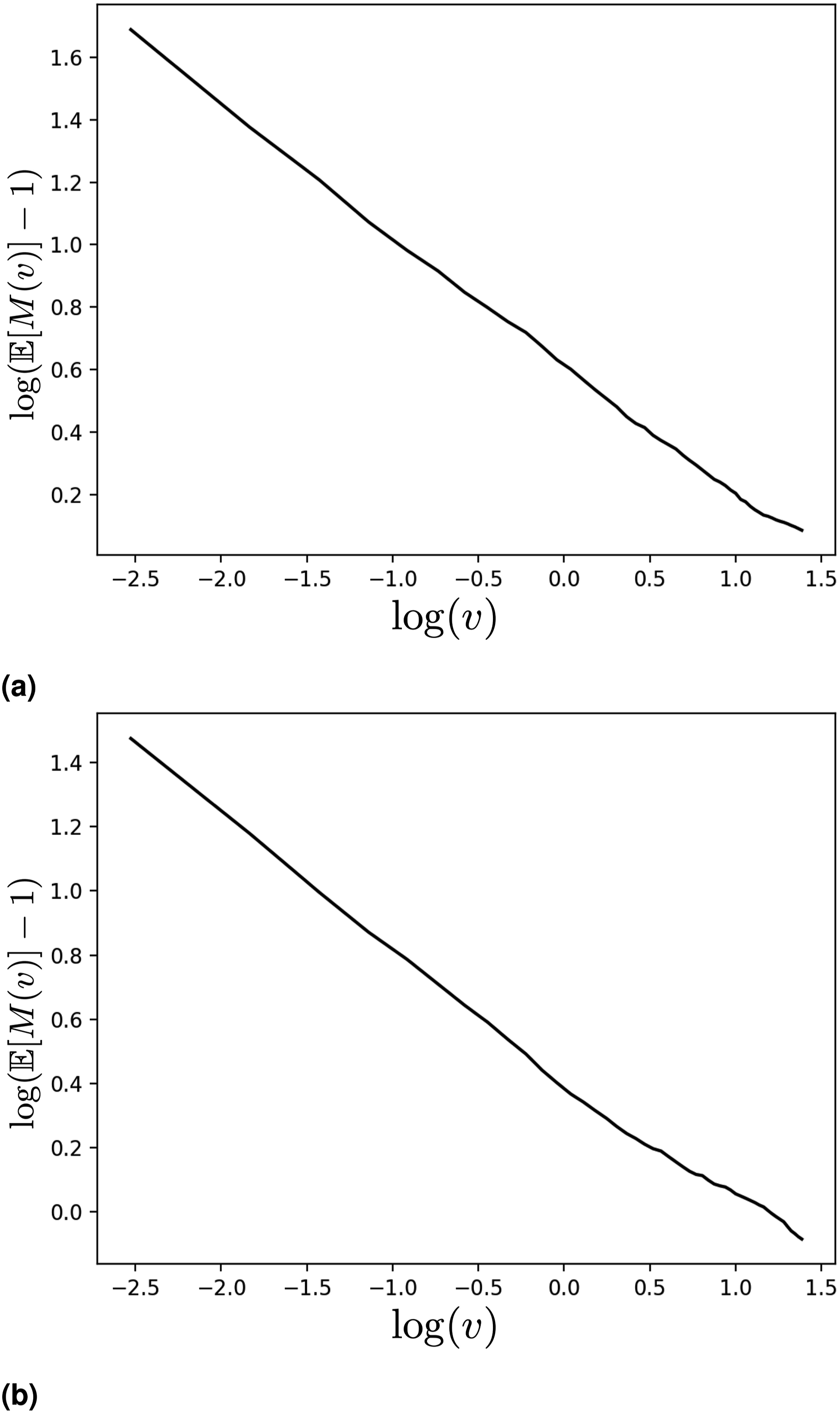$E [M (v)] - 1$ , plotted for a range of 50 speeds v from 0 (not inclusive) to 4 (inclusive), that is, v = 0.08, 0.16, …, 4.00, for two different values of t_max. Each plot done for T = 1000 trials of n = 25 random attacks (uniformly random attack times). (a) t_max = 15, n = 25, T = 1000 (b) t_max = 25, n = 25, T = 1000.

This suggests that given a particular distribution of attacks, there is some value α > 0 such that

E [M (c v)] - 1 \approx c^{α} (E [M (v)] - 1)

(15)

The slope of the line⁶ in the log-log plots in Figure 4 is −α. What α measures, roughly, is the balance of the speed-number tradeoff for the defenders: if we double the speed of the defenders, how many fewer defenders (on average) will we need to stop all the attacks? The nearly linear nature of Figure 4 indicates that, for a given (uniform in time and location) distribution of attacks, this tradeoff is roughly constant over a wide range of speeds. When α is small, it indicates that increasing the number of defenders is comparatively more important than increasing the speed (by the same proportion); in particular, if α = 1 then doubling the speed and doubling the number are equivalent.

We then examine what this α is given different distributions of attacks: for a given value of t_max, we vary the number n of attacks and see how α changes. The results are shown in Figure 5, with the y-axis being the slope of the log-log plot of the given parameters (−α, as mentioned above). Note that α < 1 in all measured cases, meaning that increasing the number of defenders by some proportion c is always more effective than increasing the speed of the defenders by a factor of c. When there are few attacks (n = 5), α ≈ 0.8, but as n increases it drops to about 0.4 before leveling out, indicating a substantial decrease in the efficacy of increasing speed as compared to increasing the number of defenders. This general pattern holds true for both plotted cases (t_max = 15 and t_max = 25) but the drop-off is sharper when t_max = 15.

Figure 5.

Relationship of −α (y-axis) to number of attacks n (x-axis) from n = 5 to n = 40, uniform attack times, for two different values of t_max. For each value of n and each of T = 1000 random attack sequences, the value M(v) was computed for 50 linearly spaced values of v from 0 to 4 (not inclusive of 0), that is, v = 0.08, 0.16, …, 4.00, and the best-fit slope of the log-log plot extracted. (a) t_max = 15 (b) t_max = 25.

6.2. Simulations for heterogeneous defenders

We conduct simulations for each of the settings from Section 2. Our experiments are run as follows:

1. Generate attacks ${(z_{j}, t_{j})}_{j = 1}^{n}$ randomly, either with fixed attack times t_j = j or uniformly random attack times in [0, t_max].

2. Compute $Opt (v, {(z_{j}, t_{j})}_{j = 1}^{n})$ for $v \in {(v_{\min}, v_{\max}]}^{m}$ , at g intervals.

3. Repeat the above for T trials and average the resulting values for each v .

We conduct all of our experiments on a circular perimeter of circumference 1, where the defenders are not permitted to leave the perimeter (so maximally distant points are at opposite ends and have distance 1/2). Comparison of the results sheds light on the conditions which favor heterogeneous defender teams and those which favor homogeneous teams and/or single super-defenders.

The structure of the simulations means each combination of defender speeds is evaluated on the same set of attack sequences, which makes the comparison fairer, and allows us to significantly speed up the computation when evaluating $Opt (v, {(z_{j}, t_{j})}_{j = 1}^{n})$ for many values of v on a single attack sequence ${(z_{j}, t_{j})}_{j = 1}^{n}$ , by exploiting the fact that Opt is a monotonically decreasing step function in v (as described in Section 4).

The full list of parameters is given in Table 3.

Table 3.

Parameters of the experiments.

Symbol	Description
m	Number of defenders (m = 2 unless specified otherwise)
n	Number of attacks
T	Number of trials
t _max	Size of attack window (not needed for heterogeneous setting (ii))
(v_min, v_max]	Range of defender speeds (inclusive of v_max but not v_min)
g	Number of speed values measured (grains) within (v_min, v_max]

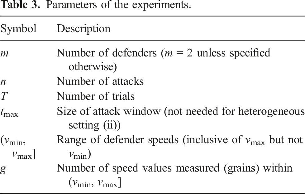
In Figure 6, we simulate sequences of n = 25 attacks of both settings, where the perimeter $X$ is a unit circle of circumference 1 and m = 2 defenders; for uniformly random attack times we set t_max = 25 to get the same density of attacks in both cases. This is analyzed over the speed range (v_min, v_max] = (0, 0.6] with g = 256 grains. The left column shows results for uniformly random

Figure 6.

2 defenders evaluated at g = 256 grains for speeds (v_min, v_max] = (0, 0.6] for 200 trials. Top row: 1 trial, front view. Middle row: 200 trials, front view. Bottom row: 200 trials, back view, showing the “ridge” at the center line v₁ = v₂ (both attack types). Left: Uniformly random attack times, n = 25, t_max = 25; Right: Fixed attack times, n = 25.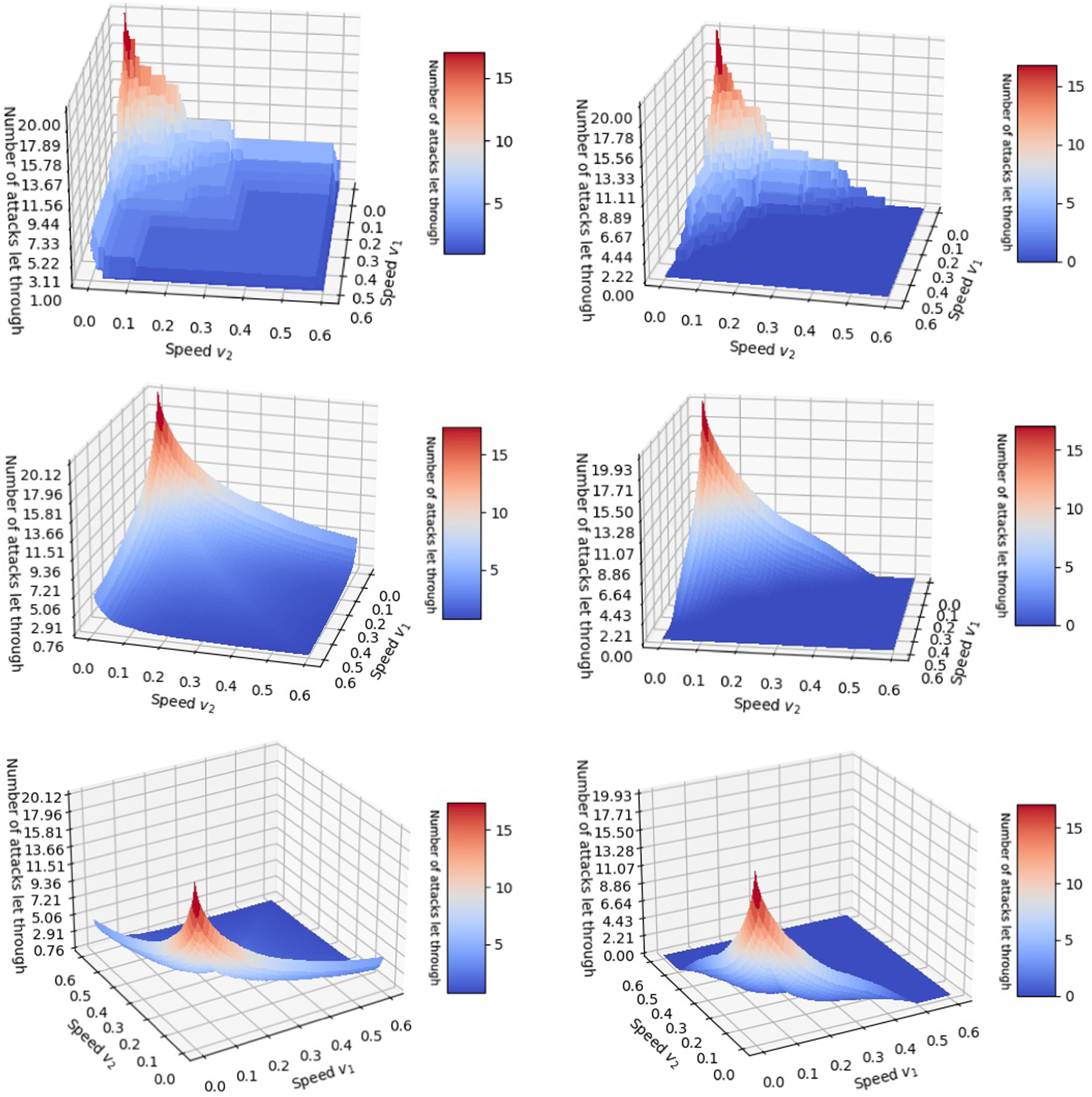

attack times; the right column shows results for fixed attack times.

The results are given as surface plots, taking defender speeds v₁, v₂ and returning Opt (v₁, v₂) (ignoring the assumption in the analysis that v₁ ≥ v₂, so the plots are symmetric about the line v₁ = v₂). We give:

• Top row: Opt (v₁, v₂) for a single sequence of attacks. This can be viewed as T = 1, and is meant to give a visualization of how adjusting the speeds of the defenders changes the ability to defend against a particular sequence. Since Opt (v₁, v₂) takes integer values, we have a monotonically decreasing step function.

• Middle and bottom rows: Opt (v₁, v₂) when averaged over T = 200 randomly generated attack sequences. Middle row gives the front view to show overall shape; bottom row gives the back view to show the ridge at v₁ = v₂. This ridge, which appears for both uniformly random attack times and fixed attack times, shows that on average homogeneous defenders are less efficient (per combined speed) than heterogeneous defenders.

From this we can make a number of interesting observations:

• Opt (v₁, v₂) is generally larger for the uniformly random attack times, as attacks which are close together in time are much harder to defend. In particular, with fixed attack times Opt (v₁, v₂) = 0 for sufficiently large defender speeds (one defender of speed 1/2 is already sufficient to defend all attacks).

• As mentioned, there is a ridge on v₁ = v₂ (the back view makes it clearly visible). This shows that on average, homogeneous defenders are less effective than well-designed heterogeneous ones.

• Under uniformly random attack times, each “half” (cutting at the v₁ = v₂ line) is empirically convex, while under fixed attack times, each “half” is convex near the v₁ = v₂ ridge but becomes concave again near the edge of the plot (as seen in the back view) and as the defender speeds increase (as can be seen on the edge in both views).

We also consider the question: what is the optimal mix of defender speeds? To answer this, we need to consider what we want to hold constant, since obviously faster defenders are always better; an obvious starting point is to look at defenders of a fixed total speed, and consider what ratio of speeds performs the best. This also means that we are comparing defender teams whose reachable sets are of equal total size (ignoring overlaps), and (because we evaluate over a grid of possible values of v ) means we compare the values of Opt( v ) on a diagonal line.

In Figure 7, we show the best (empirical) mixture: for each value of v_tot = v₁ + v₂, the returned value is $\frac{v_{2}^{*}}{v_{t o t}}$ , where

v_{2}^{*} : = \arg \min_{v_{2} \leq v_{t o t} / 2} Opt ((v_{t o t} - v_{2}, v_{2}))

(16)

Figure 7.

Empirical optimal ratio v₂/v_tot versus total speed v_tot under uniformly random (left) and fixed (right) attack times, averaged for n = 25 attacks with t_max = 25 over 200 trials.

That is, given a total speed of v_tot, what is the optimal fraction of the speed “budget” to assign to the slower defender? A value of 0.5 signifies homogeneous defenders are best; a value of 0.0 signifies that a single super-defender is best; and a value in between signify some heterogeneous mix of defenders is best.

These are based on the same experiments as shown in Figure 6. Note that the fixed attack times graph ends at v_tot = 0.5; past that, both one single super defender and homogeneous defenders will defend perfectly, so measuring the minimum no longer makes sense. However, it is striking that the benefits of a heterogeneous team persist so close to that threshold, and the optimal ratio remains relatively stable over a wide range of speed “budgets” in both settings.

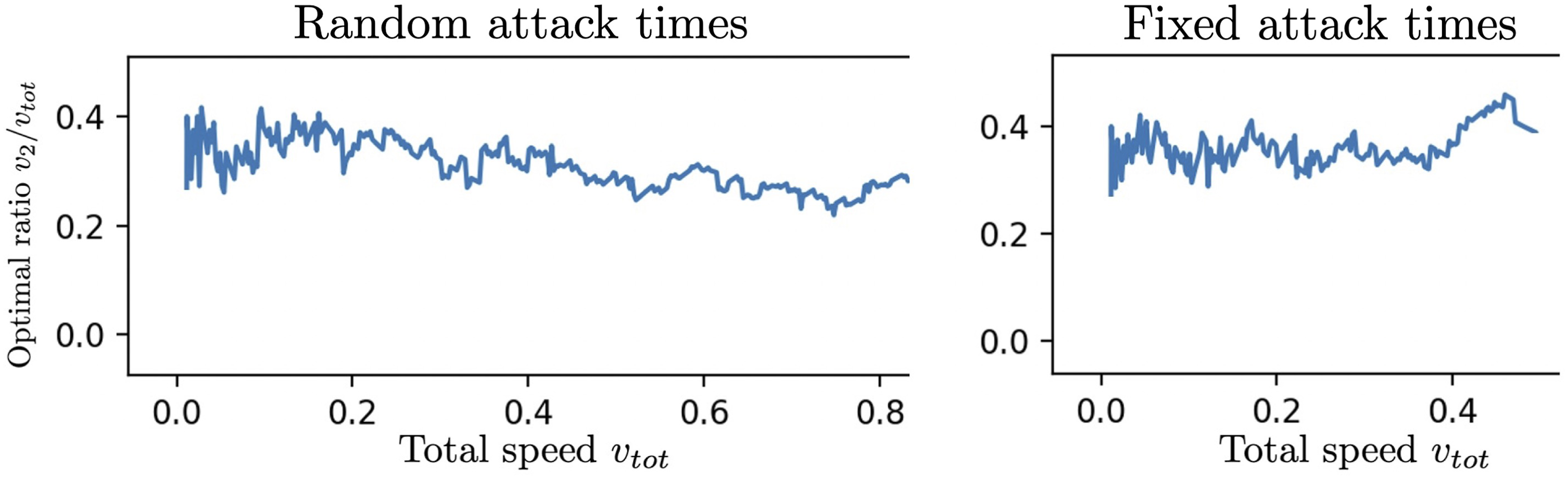
6.2.1. Computational complexity of simulations

The results of the monotonicity-based computational acceleration discussed in Section 4 can be seen in Figure 8, corresponding to the simulations shown in Figure 6. As before, the left-hand column is the results for uniformly random time attacks, and the right-hand column is the results for fixed-time attacks, while the top row represents a single trial (corresponding to the top row of Figure 8) and the bottom row correspond to the average of T = 200 trials.

Figure 8.

Monotonicity savings for the trials depicted in Figure 6. Uniformly random attack times on the left, and fixed attack times on the right. Axes labeled by position in the vector of possible speeds (0 to g − 1). Top row is for one trial (corresponding to the single trials shown in Figure 6) and bottom is average over 200 trials. Axes are labeled by grain number from 1 to 256 (linearly corresponding to speeds v₁, v₂ in Figure 6). Output in [0, 1] (depicted yellow to purple) denoting fraction of time Opt ( v , {(z_j, t_j)}) had to be computed directly (rather than known from monotonicity and previously computed values)—lower (lighter) values correspond to greater time savings from monotonicity. We denote axes in grain number since this is the relevant parameter for monotonicity savings.

Each square is a 256 × 256 grid, representing the 256² combinations of speeds v for which we want to compute Opt( v ); the shade of a given point represents the fraction of times Algorithm 2 had to be run on for that specific v (as opposed to being known already by monotonicity), running from yellow (Algorithm 2 never run) to purple (Algorithm 2 run). Note that because they represent a single trial (each), every point in the top two graphs takes a value of either 0 or 1.

We note a few things: (i) the savings increase strongly where $E [Opt (v)]$ is flatter (this is expected since $\nabla_{v} E [Opt (v)]$ corresponds to the probability that there is a step at v , and having a step nearby means the condition is less likely to be satisfied); (ii) there are darker points at regular intervals (such as in the center), which correspond to the combinations which are evaluated earlier.

Even with m = 2 and the strategic use of monotonicity, which can save up to about 95% of the running time, this can get big fairly quickly.

6.2.2. Simulations for unit horizon

Simulation results for the case of two defenders on a circular perimeter with unit horizon are shown in Figure 9. Note that in this case, heterogeneity is not beneficial, it is even detrimental. The optimal speed allocation is to assign the entire speed budget to one defender or split it equally.

Figure 9.

Unit-horizon case, 2 defenders evaluated at g = 128 grains for speeds (v_min, v_max] = (0, 0.5] for 10,000 trials and n = 25 attacks. Color bar corresponds to average of Opt( v ). Top: back view, note the lack of the “ridge” seen in Figure 6. Bottom: front view.

7. Conclusion

We introduced and studied a minimal model to map out how and why heterogeneity in robotic teams affects performance in perimeter defense applications.

In the case of homogeneous defenders, our results show a preference for a larger number of slower robots instead of a smaller number of quicker robots. The resulting multi-robot setting then raises the question if heterogeneity in the team composition is beneficial or detrimental. Thus, we also investigated the heterogeneous setting.

On the one hand, we showed that a heterogeneous team achieves better performance when full information of the oncoming attacks is available to the defenders. Moreover, we uncovered a seemingly universal behavior, where the ratio of optimal defender speeds is nearly constant for a range of problem parameters.

On the other hand, we proved that heterogeneity is detrimental to the system’s performance in the converse case where minimal attack information is available. These results suggest that heterogeneity is potentially a non-robust property, since less system information dramatically decreases its usefulness.

Future directions involve quantifying and studying the use of heterogeneity when intermediate levels of information are available to the defenders. This would explore the existence of a phase transition where heterogeneity changes from decreasing to improving system performance. Possible scenarios include varying the horizon length of incoming attacks between the cases of 1 and ∞ considered in the paper. Another scenario augments the unit-time horizon with the knowledge of the number of remaining attacks. In particular, we conjecture that even in this case defenders should always capture attacks if possible and that heterogeneity remains detrimental. Lastly, we wish to perform numerical simulations for a larger number of defenders.

Footnotes

Author’s note

Sukhatme holds concurrent appointments as a Professor at USC and as an Amazon Scholar. This paper describes work performed at USC and is not associated with Amazon.

Declaration of conflicting interests

The author(s) declared no potential conflicts of interest with respect to the research, authorship, and/or publication of this article.

Funding

The author(s) disclosed receipt of the following financial support for the research, authorship, and/or publication of this article: This work was supported by Army Research Laboratory.

ORCID iDs

Aviv Adler

Oscar Mickelin

Ragesh K. Ramachandran

Notes

Proof of Theorem 1

In this proof, for readability we denote i*≔i*( j ) and j*≔j*( j ); these values depend on j (and are important to keep track of to reconstruct the optimal defense plan ℓ ).

Algorithm 1 depends on the function $V (j) : {0, 1, \dots, n}^{m} \to N$ , which denotes the following: suppose that defender i (with speed v_i) is required to thwart attack j_i and then no others after that (but defender i can thwart attacks arriving before $t_{j_{i}}$ , and if j_i = 0, then defender i is not allowed to thwart any attack); V( j ) is the minimum number of defenders that can be let through under these constraints. Then the following hold:

• V (0, …, 0) = n (the base case from which we recursively compute V);

• $Opt (v, {(z_{j}, t_{j})}_{j = 1}^{n}) = \min_{j} V (j)$ (this allows us to extract the correct value by keeping track of this minimum).

We then want to recursively compute V( j ) for all j ∈ {0,1,…,n}^m. This can be done by considering (17)

S = \arg \max_{i \in [m]} j_{i}

that is, the set of defenders that thwart the latest attack in j . We then (arbitrarily) select a defender

i^{*} \in S

to consider.

We can then ask: suppose j′ is the last attack that defender i* thwarts before thwarting $j_{i^{*}}$ . Then $j^{'} < j_{i^{*}}$ and $1_{i^{*}} (j^{'}, j_{i^{*}}) = 1$ , since otherwise i* cannot defend both attacks. The best the defenders can do in this case is to thwart $V (j_{- i^{*}} (j^{'}))$ attacks, then have defender i* thwart $j_{i^{*}}$ : if $| S | = 1$ (i* is the unique defender required to thwart $j_{i^{*}}$ ) then this is 1 more attack thwarted in total; otherwise it’s redundant. Thus, minimizing over all possible j′, we have (18)

\begin{array}{l} V (j) = \min_{j^{'}} {V (j_{- i^{*}} (j^{'})) : j^{'} < j_{i^{*}} and \\ 1_{i^{*}} (j^{'}, j_{i^{*}}) = 1} + 1 {| S | = 1} \end{array}

(where

1 {| S | = 1}

is the indicator function for

| S | = 1

). We also let j* be (any) j′ which minimizes this, which will be important for reconstructing the optimal defense plan ℓ . By iterating over all j in lexicographic order, we can compute V( j ) using the above recursion (and starting from V (0, …, 0) = n). We keep track of the minimum value (and the j ^min which minimizes V( j )) and output this as

Opt (v, {(z_{j}, t_{j})}_{j = 1}^{n})

. To reconstruct the defense plan, we start with j ^min and read backward: we know that the optimal defense plan (which is the optimal defense plan for j ^min) starts by defending according to

j_{i^{*}}^{\min} (j^{*})

and then having i* defend

j_{i^{*}}^{\min}

at the end; we then recurse to

j_{i^{*}}^{\min} (j^{*})

until we arrive at j = (0, …, 0).

Proof of Proposition 1

Our setup is: the defenders are currently at a distance a and an attack comes in at x which can be reached by at least one of the defenders, after which N further (uniformly and randomly distributed) attacks will follow. We have two policies: f′, which declines to capture in this case, and f*, which follows the conjectured optimal strategy of always capturing, and always maximizing the distance between the defenders conditional on whether or not a capture is made.

We let J_f′(a; x; N) be the expected reward of following policy f′ from the given conditions (current separation a, attack at x, N attacks after that), and $J_{f^{*}} (a; x; N)$ be the policy of following f* (including the initial capture which f′ does not do). Then if we can show that $J_{f^{'}} (a; x; N) \leq J_{f^{*}} (a; x; N)$ it proves that f* outperforms all policies which do not make the capture at the current time. Since our result is such that if it works for this value of N, it also works for smaller values of N, it means that the optimal policy must always capture if possible and thus, by Proposition 2 in the main work, the policy f* is therefore optimal under the given conditions.

We also assume that the current separation between the defenders (before deciding whether to thwart the current reachable attack) is a ≥ 2v₂; this assumption is justified because by Proposition 2 in the main work, we know that all things equal we want to maximize separation (J is monotonic in a), and 2v₂ separation can always be maintained even when capturing since the non-capturing defender can always maximize its distance to the current attack; even if the initial position of the defenders does not satisfy this, after 2 attacks it can always be achieved (even with captures).

We assume that 2v₁ ≤ 1 and v₁ + 3v₂ ≤ 1 (otherwise by Theorem 2 from the main work it is possible to thwart all attacks no matter what, which by definition means the optimal policy thwarts the current attack).

Let s_f′(i) and $s_{f^{*}} (i)$ be the expected sizes of the union of the reachable set at step i after the current step, under policies f′ and f*, respectively, where f′ does not thwart the attack and f* is the conjectured optimal policy. Then s_f′(i) ≤ min (1, 2 (v₁ + v₂)) and $s_{f^{*}} (i) \geq \max (2 v_{1}, v_{1} + 3 v_{2})$ . The first inequality is a generic upper bound on the size of the reachable set union for defenders of speeds v₁, v₂; the second holds because if no capture is made, the defenders can achieve at least v₁ + v₂ separation, and if a capture is made, they can achieve at least 2v₂ separation (the non-capturing defender maximizes separation), in which case the union of the reachable sets satisfies the given bound.

Thus, the probability that the attack at step i is reachable (with the current attack considered step 0) is bounded by the above, and hence (19)

\begin{array}{l} J_{f^{'}} (a; x; N) & \leq \min (1, 2 (v_{1} + v_{2})) N \end{array}

(20)

\begin{array}{l} and J_{f^{*}} (a; x; N) & \geq 1 + \max (2 v_{1}, v_{1} + 3 v_{2}) N \end{array}

Subtracting using these bounds, we get that (21)

\begin{array}{l} J_{f^{*}} (a; x; N) - J_{f^{'}} (a; x; N) \\ \geq 1 - \min (1 - 2 v_{1}, 1 - v_{1} - 3 v_{2}, 2 v_{2}, v_{1} - v_{2}) N \\ = 1 - w N \geq 0, if N \leq \frac{1}{w} . \end{array}

The extra “+1” comes from the fact that f* makes a capture at the current step, while f′ does not. Thus, we are done.

Note that the bound in the Proposition is not the best possible. We can sharpen it by noting that under f*, when a capture is not made, the union of the reachable sets on the next step is min (1, 2 (v₁ + v₂)) (maximizing separation without needing to capture allows the defenders to have non-intersecting reachable sets). We leave the improvements to future work.

Proof of Proposition 2

We next proceed with the proof of Proposition 2 in the main text.

The proof is by induction on the number of attacks N. We show (ii) together with the following additional properties:

(iii) For any N, J (a; N) is an increasing function of a;

We start with the base case N = 0. Note that given an initial defender distance a, the probability that the first attack can be defended is just the size of the union of the interval [−v₁, v₁] (where the faster defender can reach) with the interval [a − v₂, a + v₂] (where the slower defender can reach). We denote the size of this union as

s (a) : = s (a, v_{1}, v_{2}) : = {\begin{cases} 2 v_{1}, for a \leq v_{1} - v_{2} \\ \min (v_{1} + v_{2} + a, 2 (v_{1} + v_{2}), 1), \\ for a > v_{1} - v_{2} \end{cases}

Clearly, J (a; 0) ≤ s(a), with equality if (i) holds. Since s(a) is a monotonically increasing function for a ∈ [0, 1/2], (ii) holds. Clearly, J (a; 0) = s(a), so (iii) holds as well.

Next, we proceed with the induction step and show (ii). We make use of the following recursive formula: (22)

J (a; N + 1) = s (a) + E_{x} [J (f (a, x); N)]

which holds since attack N + 1 is defended with probability s(a), by (i), and by independence of the distributions of the attacks. Since J (·; N) is an increasing function, by (iii), this expression is maximized by an f maximizing f (a, x, N), subject to the constraint in (i). Equation (22) also shows (iii), as J (a; N + 1) is the sum of two increasing functions. This concludes the induction step and therefore the proof.

Proof of Theorem 2

Analysis of cost minimization extension for homogeneous defenders

In Section 4, inspired by the work of Velhal et al. (2022),⁷ we showed an extension of Algorithm 1 which both finds the minimum number M of defenders needed to intercept all the attacks and also finds the assignment of those M defenders to the n attacks ${(z_{j}, t_{j})}_{j = 1}^{n}$ that minimizes a given linear cost objective function. This cost is represented by values c_j,j′ ≥ 0 for all pairs j, j′ such that attack j′ is reachable from attack j, that is, such that dist (z_j, z_j′) ≤ v (t_j′ − t_j); Velhal et al. (2022) focus on a special objective of the form (27)

c_{j, j^{'}} \propto dist (z_{j}, z_{j^{'}})

which represents the fuel needed to travel from z_j to z_j′. One other small difference is that their formulation includes reserve stations, at which the defenders start; our original formulation of the homogeneous perimeter defense problem given in Section 3 does not include this, as it does not affect the minimum number of defenders needed to thwart all the attacks.

They also split their method into two parts:

(a) Fixing the number (and origin) of the defenders, find the assignment of defenders to attacks which minimizes the fuel cost. This is done by formulating a Linear Sum Assignment Problem (LSAP, as given in [equation (10)-(10e), Velhal et al. (2022)]), which is then solved by known techniques. If no such solution exists, then it will find the cost-minimizing assignment that thwarts the maximum possible number of attacks.

(b) Determine the minimum number of defenders needed to defend all attacks, which is done by analyzing the output of the LSAP and either adding defenders if there were undefended attacks or removing them if there were idle defenders in the optimal solution of the LSAP. This is given in [Algorithm 1, Velhal et al. (2022)].

In [Section 3.2, Velhal et al. (2022)], it is claimed that [Algorithm 1, Velhal et al. (2022)] computes the minimum number of defenders required to neutralize all the intruders. However, we believe that there are examples where [Algorithm 1, Velhal et al. (2022)] does not successfully find the minimum number of defenders.

First, it is asserted in [Algorithm 1, Velhal et al. (2022)] (lines 11-12) that “if All defender are assigned to task then Solution is optimal.” The algorithm terminates under this condition. This assertion is, however, not proven in their work, and furthermore seems to fail, such as in the following example:

• The perimeter is the square {(x, y): |x|, |y| ≤ 1}, with a defender reserve station at (0, 0). All defenders have speed 1.

• 10 attacks occur at the following times and locations on the perimeter: 5 attacks at (0, 1) at times 2, 6, 10, 14, 18; and 5 attacks at (1, 0) at times 4, 8, 12, 16, 20.

To minimize the fuel cost for 2 defenders, one should be sent to (0, 1) (arriving at time 1) and wait there, neutralizing all attacks at that location; and the other to (1, 0) (also arriving at time 1 and neutralizing all attacks at that location). This yields a total cost of 2, and assigns each defender at least one task. However, the problem can be solved by one defender by alternating between (0, 1) and (1, 0) (requiring a total cost of $1 + 9 \sqrt{2}$ but only one defender). Thus, even though the optimal solution for the 2-defender case assigned all defenders to tasks, the minimum number of defenders required is only 1.

Additionally, it is claimed that if the optimal solution to the LSAP with m defenders leaves q attacks undefended, then the minimum number of defenders needed to defend all the attacks will be M = m + q; this is used in line 8 of [Algorithm 1, Velhal et al. (2022)]. This claim is substantiated by [Theorem 1, Velhal et al. (2022)], which asserts that adding another defender can only neutralize one additional attack, while all other undefended attacks remain infeasible.

However, a similar counterexample as above seems to show that this is not the case. Consider the above counterexample, but where the defenders have only speed 1/2 (sufficient to arrive at (0, 1) by time 2 from the reserve, but insufficient to traverse the $\sqrt{2}$ distance between (0, 1) and (1, 0) in 2 units of time). Let the 10 attacks be labeled with j = 1, 2, …, 10, that is, attack j arrives at time 2j, and at (0, 1) if j is odd. Then according to the LSAP formulation from Velhal et al. (2022), the cost incurred by requiring a defender to go from attack k to attack j > k is (28)

c_{k, j}^{s} = {\begin{cases} 0 & if j \equiv k \mod (2) \\ κ & otherwise \end{cases}

where κ is a large value intended to penalize time-infeasible assignments (given in [equation (5), Velhal et al. (2022)]). However, since all attacks j must be neutralized in the LSAP, this means that the defender must neutralize the attacks in order of time (or else incur infinite penalty for defending attacks out of time order, as specified in [equation (5), Velhal et al. (2022)]); thus, only the first attack can be defended, with the other 9 incurring cost κ. According to [Theorem 1, Velhal et al. (2022)]: “If one reserve defender is added to the team of defenders, then only one previously time-infeasible intruder will get assigned with time feasibility. All other (q − 1) time-infeasible assignments remain time-infeasible.” However, in this example, adding an additional defender allows all intruders to become time-feasible, as one defender can move to (0, 1) and the other can move to (1, 0).

Therefore, it appears that [Algorithm 1, Velhal et al. (2022)] will not always find the minimum number of defenders.

Finally, however, we note that since the solution to the LSAP does indicate whether the problem is feasible for the given number of defenders, it is possible to use O (log n) calls of the LSAP to find the minimum number of defenders needed by using a binary search (thus taking a total of O (n³ log n) time).

References

Adler

Mickelin

Ramachandran

, et al. (2023) The role of heterogeneity in autonomous perimeter defense problems. In: Algorithmic Foundations of Robotics XV. Cham: Springer International Publishing, 115–131.

Bajaj

Bopardikar

(2019) Dynamic boundary guarding against radially incoming targets. In: 2019 IEEE 58th conference on decision and control (CDC), Nice, 11–13 December 2019, 4804–4809. IEEE.

Casey

(2014) Drones Bring Fight and Flight to Battle against Poachers. New York, NY: Scientific American. (online) 20.

Chopra

Egerstedt

(2014) Heterogeneous multi-robot routing. In: 2014 American control conference, Portland, OR, 04–06 June 2014, 5390–5395. IEEE.

Cohen

(2007) Natural disasters. Drone spy plane helps fight California fires. Science 318(5851): 727.

Cormen

Leiserson

Rivest

, et al. (2001) Introduction to Algorithms. 2nd edition. Cambridge, MA: The MIT Press.

Fuchs

Khargonekar

Evers

(2010) Cooperative defense within a single-pursuer, two-evader pursuit evasion differential game. In: 49th IEEE conference on decision and control (CDC), Atlanta, GA, 15–17 December 2010, 3091–3097.

Guerrero-Bonilla

Nieto-Granda

Egerstedt

(2021) Robust perimeter defense using control barrier functions. In: 2021 international symposium on multi-robot and multi-agent systems (MRS), Cambridge, 04-05 November 2021, 164–172. IEEE.

Isaacs

(1965) Differential games: a mathematical theory with applications to warfare and pursuit, control and optimization. In: SIAM Series in Applied Mathematics. Hoboken, NJ: Wiley.

10.

Lee

Shishika

Kumar

(2020) Perimeter-defense game between aerial defender and ground intruder. In: 2020 59th IEEE conference on decision and control (CDC), Jeju, 14–18 December 2020, 1530–1536.

11.

Lykou

Moustakas

Gritzalis

(2020) Defending airports from UAS: a survey on cyber-attacks and counter-drone sensing technologies. Sensors 20(12): 3537.

12.

Macharet

Chen

Shishika

, et al. (2020) Adaptive partitioning for coordinated multi-agent perimeter defense. In: 2020 IEEE/RSJ international conference on intelligent robots and systems (IROS), Las Vegas, NV, 24 October 2020–24 January 2021, 7971–7977. IEEE.

13.

Mayya

Ramachandran

Zhou

, et al. (2022) Adaptive and risk-aware target tracking for robot teams with heterogeneous sensors. IEEE Robotics and Automation Letters 7(2): 5615–5622.

14.

Puterman

(2014) Markov Decision Processes: Discrete Stochastic Dynamic Programming. Hoboken, NJ: John Wiley & Sons.

15.

Ramachandran

Preiss

Sukhatme

(2019) Resilience by reconfiguration: exploiting heterogeneity in robot teams. In: 2019 IEEE/RSJ international conference on intelligent robots and systems (IROS), Macau, 03–08 November 2019, 6518–6525.

16.

Ramachandran

Pierpaoli

Egerstedt

, et al. (2022) Resilient monitoring in heterogeneous multi-robot systems through network reconfiguration. IEEE Transactions on Robotics 38(1): 126–138.

17.

Ravichandar

Shaw

Chernova

(2020) STRATA: unified framework for task assignments in large teams of heterogeneous agents. Autonomous Agents and Multi-Agent Systems 34(38): 38.

18.

Santos

Egerstedt

(2018) Coverage control for multi-robot teams with heterogeneous sensing capabilities using limited communications. In: 2018 IEEE/RSJ international conference on intelligent robots and systems (IROS), Madrid, 01–05 October 2018, 5313–5319.

19.

Shishika

Kumar

(2018) Local-game decomposition for multiplayer perimeter-defense problem. In: 2018 IEEE conference on decision and control (CDC), Miami, FL, 17–19 December 2018, 2093–2100.

20.

Shishika

Kumar

(2020) A review of multi agent perimeter defense games. In: Decision and Game Theory for Security. Berlin: Springer International Publishing, 472–485.

21.

Shishika

Paulos

Dorothy

, et al. (2019) Team composition for perimeter defense with patrollers and defenders. In: 2019 IEEE 58th conference on decision and control (CDC), Nice, 11–13 December 2019, 7325–7332.

22.

Shishika

Paulos

Kumar

(2020) Cooperative team strategies for multi-player perimeter-defense games. IEEE Robotics and Automation Letters 5(2): 2738–2745.

23.

Smith

Bopardikar

Bullo

(2009) A dynamic boundary guarding problem with translating targets. In: Proceedings of the 48h IEEE conference on decision and control (CDC) held jointly with 2009 28th Chinese control conference, Shanghai, 15–18 December 2009, 8543–8548. IEEE.

24.

Twu

Mostofi

Egerstedt

(2014) A measure of heterogeneity in multi-agent systems. In: 2014 American control conference, Portland, OR, 04–06 June 2014, 3972–3977.

25.

Velhal

Sundaram

Sundararajan

(2022) Dynamic resource allocation with decentralized multi-task assignment approach for perimeter defense problem. IEEE Transactions on Aerospace and Electronic Systems 58(4): 3313–3325.

26.

Von Moll

Garcia

Casbeer

, et al. (2020) Multiple-pursuer, single-evader border defense differential game. Journal of Aerospace Information Systems 17(8): 407–416.

27.

Yan

Shi

Zhong

(2019) Reach-avoid games with two defenders and one attacker: an analytical approach. IEEE Transactions on Cybernetics 49(3): 1035–1046.

28.

Zych

(2020) The development of the israeli national missile defense concept. Kwartalnik Bellona 701(2): 75–88.