
Abstract
Motion planning can be cast as a trajectory optimisation problem where a cost is minimised as a function of the trajectory being generated. In complex environments with several obstacles and complicated geometry, this optimisation problem is usually difficult to solve and prone to local minima. However, recent advancements in computing hardware allow for parallel trajectory optimisation where multiple solutions are obtained simultaneously, each initialised from a different starting point. Unfortunately, without a strategy preventing two solutions to collapse on each other, naive parallel optimisation can suffer from mode collapse diminishing the efficiency of the approach and the likelihood of finding a global solution. In this paper, we leverage on recent advances in the theory of rough paths to devise an algorithm for parallel trajectory optimisation that promotes diversity over the range of solutions, therefore avoiding mode collapses and achieving better global properties. Our approach builds on path signatures and Hilbert space representations of trajectories and connects parallel variational inference for trajectory estimation with diversity-promoting kernels. We empirically demonstrate that this strategy achieves lower average costs than competing alternatives on a range of problems, from 2D navigation to robotic manipulators operating in cluttered environments.
1. Introduction
Trajectory optimisation is one of the key tools in robotic motion, used to find control signals or paths in obstacle-cluttered environments that allow the robot to perform desired tasks. These trajectories can represent a variety of applications, such as the motion of autonomous vehicles or robotic manipulators. In most problems, we consider a state-space model, where each distinct situation for the world is called a state, and the set of all possible states is called the state space (LaValle, 2006). When optimising candidate trajectories for planning and control, two criteria are usually considered: optimality and feasibility. Although problem dependant, in general, the latter evaluates in a binary fashion whether the paths generated respect the constraints of both the robot and the task, such as physical limits and obstacle avoidance. Conversely, optimality is a way to measure the quality of the generated trajectories with respect to task-specific desired behaviours. For example, if we are interested in smooth paths, we will search for trajectories that minimise changes in velocity and/or acceleration. The complexity of most realistic robot planning problems scales exponentially with the dimensionality of the state space and is countably infinite. When focusing on motion planning, a variety of algorithms have been proposed to find optimal and feasible trajectories. These can be roughly divided into two main paradigms: sampling-based and trajectory optimisation algorithms.
Sampling-based planning (Gammell and Strub, 2021) is a class of planners which rely on a sampling procedure to compose paths. In many cases, these approaches will be probabilistically complete and asymptotically optimal with respect to given optimality criteria (Al-Bluwi et al., 2012). These approaches decompose the planning problem into a series of sequentially sampled next steps evaluated via a tree-based (LaValle and Kuffner, 2001) or graph-based (Jaillet and Simeon, 2008; Kavraki et al., 1996) approach. However, most approaches are limited in their ability to encode kinodynamic cost like trajectory curvature (Heilmeier et al., 2020) or acceleration torque limits (Berntorp et al., 2014). In addition, despite the completeness guarantee, sampling-based planners are often more computationally expensive as the search space grows and can obtain highly varying results due to the random nature of the algorithms.
Trajectory optimisation algorithms (Gonzalez et al., 2016) use different techniques to minimise a cost functional that encourages solutions to be both optimal and feasible. The most direct optimisation procedure relies on a differentiable cost function and uses functional gradient techniques to iteratively improve the trajectory quality (Ratliff et al., 2009). However, many different strategies have been proposed. For example, one may start from a randomly initialised candidate trajectory and proceed by adding random perturbations to explore the search space and generate approximate gradients, allowing any arbitrary form of cost functional to be encoded (Kalakrishnan et al., 2011). The same approach can be used to search for control signals and a local motion plan concurrently (Williams et al., 2016). Finally, a locally optimal trajectory can also be obtained via decomposing the planning problem with sequential quadratic programming (Schulman et al., 2013). A drawback of these methods is that they usually find solutions that are locally optimal and may need to be run with different initial conditions to find solutions that are feasible or with lower costs Figure 1. An episode of the Kitchen scene. Depicted is one of the collision-free paths found by SigSVGD on a reaching task using a 7-DOF Franka Panda arm on the MotionBenchMaker planning benchmark.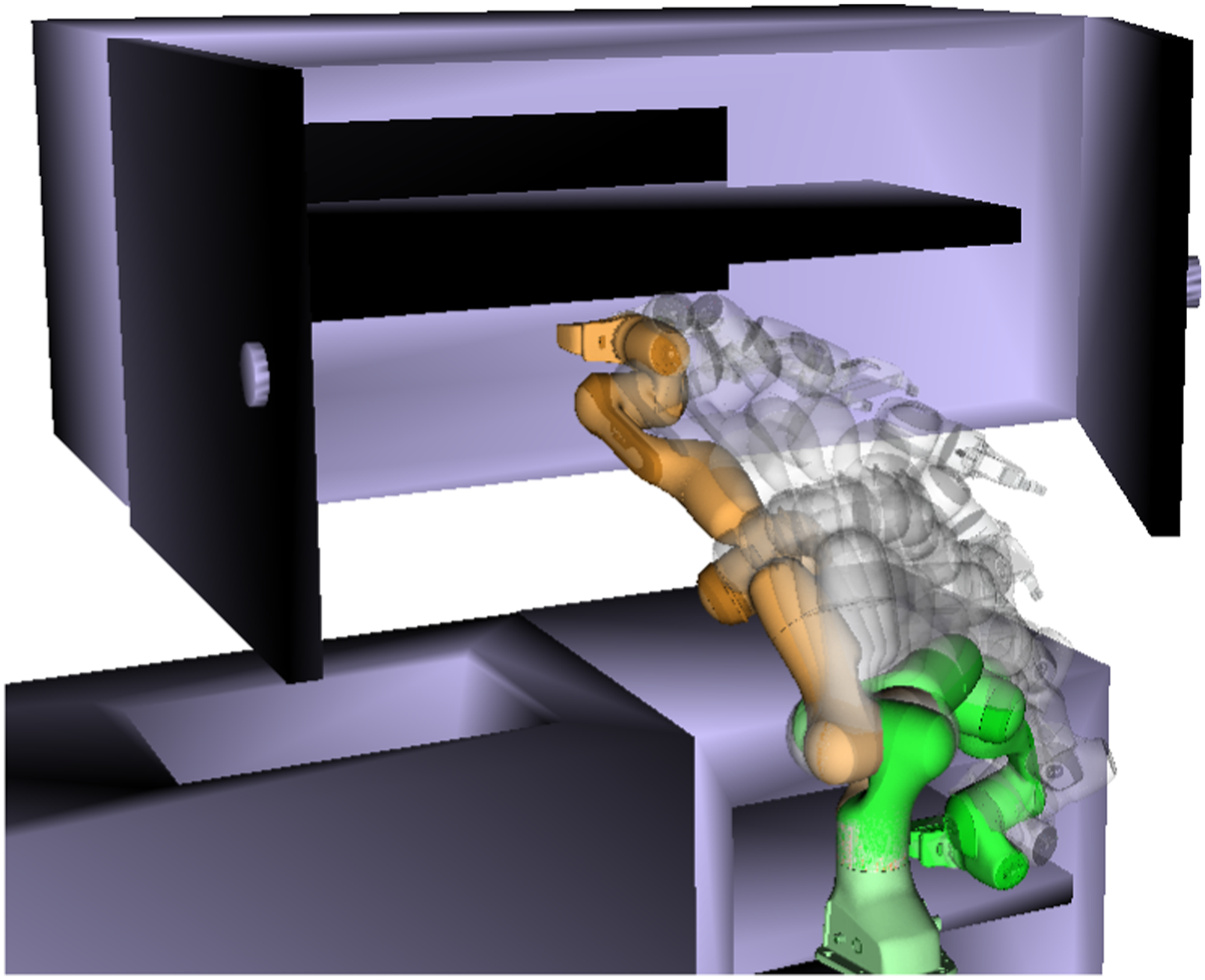
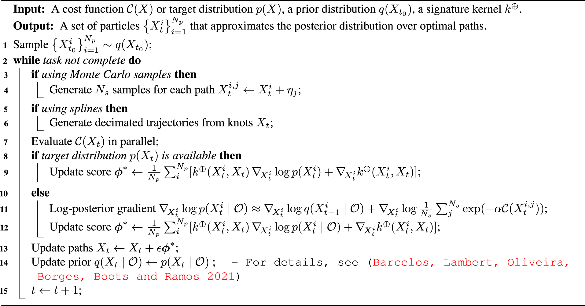
Our goal with the present work is to propose a new trajectory optimisation method to improve path diversity. More specifically, we focus on a class of algorithms that performs parallel trajectory optimisation of a batch of trajectories. This concurrent optimisation of several paths in itself already alleviates the proneness to local minima since many initial conditions are evaluated simultaneously. Nonetheless, we show how a proper representation of trajectories when performing functional optimisation leads to increased diversity and solutions with a better global property, either with direct gradients or Monte Carlo-based gradient approximations. For an illustrative example, refer to Figure 2. Qualitative analysis of 2D planning task. The plot shows the final 20 trajectories found with different optimisation methods. The colour of each path shows its normalised final cost. Note how all batch gradient descent trajectories converge to two modes of similar cost. Paths found by SVMP are already more diverse, but one of the gradient descent modes is lost. Note how when multiple trajectories converge to a single trough, the knots are pushed away by the repulsive force resulting in suboptimal solutions. Conversely, paths found by SigSVGD are diverse and able to find more homotopic solutions, including those found by BGD. Note also how paths are able to converge to the same trough without being repelled by one another since the repulsive force takes into account the entire trajectory and not exclusively the spline knot placement. That also allows for paths that are more direct and coordinated than SVMP.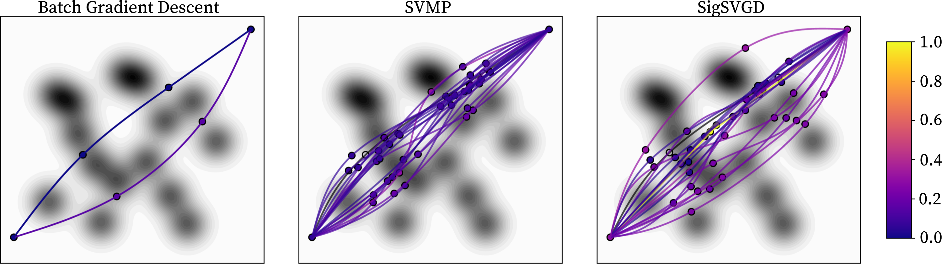
Our approach is based on two cornerstones. On one hand, we use a modification of Stein Variational Gradient Descent (SVGD) (Liu and Wang, 2016), a variational inference method to approximate a posterior distribution with an empirical distribution of sampled particles, to optimise trajectories directly on a structured Reproducing Kernel Hilbert Space (RKHS).
The structure of this space is provided by the second pillar of our approach. We leverage recent advancements in rough path theory to encode the sequential nature of paths in the RKHS using a Path Signature Kernel (Kiraly and Oberhauser, 2019; Salvi et al., 2021). Therefore, we can approximate the posterior distribution over optimal trajectories with structured particles during the optimisation while still taking into account motion planning and control idiosyncrasies.
More concretely, the main contributions of this paper are listed below: We introduce the use of path signatures (Lyons, 2014) as a canonical feature map to represent trajectories over high-dimensional state spaces. Next, we outline a procedure to incorporate the signature kernel into a variational inference framework for motion planning. Finally, we demonstrate through experiments in both planning and control that the proposed procedure results in more diverse trajectories, which aid in avoiding local minima and lead to a better optimisation outcome.
The paper is organised as follows. In Section 2, we review related work, contrasting the proposed method to the existing literature. In Section 3, we provide background on path signatures and motion planning as variational inference, which are the foundational knowledge for the method outlined in Section 4. Finally, in Section 5, we present a number of simulated experiments, followed by relevant discussions in Section 6.
2. Related work
Trajectory optimisation refers to a class of algorithms that start from an initial sub-optimal path and find a, possibly local, optimal solution by minimising a cost function. Given its broad definition, there are many seminal works in the area. One influential early work is Covariant Hamiltonian Optimisation for Motion Planning (CHOMP) (Ratliff et al., 2009) and related methods (Zucker et al., 2013; Byravan et al., 2014; Marinho et al., 2016). The algorithm leverages the covariance of trajectories coupled with Hamiltonian Monte Carlo to perform annealed functional gradient descent. However, one of the limitations of CHOMP and related approaches is the need for a fully-differentiable cost function.
In Stochastic Trajectory Optimisation for Motion Planning (STOMP) (Kalakrishnan et al., 2011), the authors address this by approximating the gradient from stochastic samples of noisy trajectories, allowing for non-differentiable costs. Another approach used in motion planning is quality diversity algorithms, at the intersection of optimisation and evolutionary strategies, of which Covariance Matrix Adaptation Evolution Strategy (CMA-ES) is the most prominent (Hansen et al., 2003; Hämäläinen et al., 2020; Tjanaka et al., 2022). CMA-ES is a derivative-free method that uses a multivariate normal distribution to generate and update a set of candidate solutions, called individuals. The algorithm adapts the covariance matrix of the distribution based on the observed fitness values of the individuals and the search history, balancing exploration and exploitation of the search space. Because of its stochastic nature, it is ergodic and copes well with multi-modal problems. Nonetheless, it may require multiple initialisations, and it typically requires more evaluations than gradient-based optimisers (Hansen, 2016).
TrajOpt (Schulman et al., 2013), another prominent planner, adopts a different approach solving a sequential quadratic program and performing continuous-time collision checking. Contrary to sampling-based planners, these trajectory optimisation methods are fast but only find locally optimal solutions and may require reiterations until a feasible solution is found. Another issue common to these approaches is that, in practice, they require a fixed and fine parametrisation of trajectory waypoints to ensure feasibility and smoothness, which negates the benefit of working on continuous trajectory space. To address this constraint, in Marinho et al. (2016), the authors restrict the optimisation and trajectory projection to an RKHS with an associated squared-exponential kernel. However, the cost between sparse waypoints is ignored, and the search is still restricted to a deterministic trajectory. Another approach was proposed in GPMP (Dong et al., 2016; Mukadam et al., 2017; Mukadam et al., 2018) by representing trajectories as Gaussian Processes (GP) and looking for a maximum a posteriori (MAP) solution of the inference problem.
More closely related to our approach are Lambert and Boots (2021) and Yu and Chen (2022) which frame motion planning as a variational inference problem and try to estimate the posterior distribution represented as a set of trajectories. In Yu and Chen (2022), the authors modify GPMP with a natural gradient update rule to approximate the posterior. On the other hand, in Stein Variational Motion Planning (SVMP) (Lambert and Boots, 2021), the posterior inference is optimised using Stein variational gradient descent. This method is similar to ours, but the induced RKHS does not take into account the sequential nature of the paths being represented but rather treats paths similar to static vectors on a high-dimensional space. This approach leads to a diminished repulsive force and lack of coordination along the dimensions of the projected space.
In contrast, our approach—which we will refer to as Kernel Signature Variational Gradient Descent (SigSVGD)—uses the path signature to encode the sequential nature of the functional being optimised. We argue that this approach leads to a better representation of trajectories promoting diversity and finding better local solutions. To empirically corroborate this claim, we use Occam’s razor principle and take SVMP as the main baseline of comparison since it more closely approximates our method.
We note that the application of trajectory optimisation need not be restricted to motion planning. By removing the constraint of a target state and making the optimisation process iterative over a rolling horizon, we retrieve a wide class of Model Predictive Controllers with applications in robotics (Barcelos et al., 2021; Barcelos et al., 2020; Lambert et al., 2020; Williams et al., 2016). Stein Variational MPC (SVMPC) (Lambert et al., 2020) uses variational inference with SVGD optimisation to approximate a posterior over control policies and more closely resembles SigSVGD. However, like SVMP, it too does not take into account the sequential nature of control trajectories, and we will illustrate how our approach can improve the sampling of the control space and promote better policies.
3. Background
3.1. Trajectory optimisation in robotics
Consider a system with state

Finally, we draw the reader’s attention to the fact that the problem stated in equation (1) can be viewed as an open-loop optimal control problem. If the solution can be found in a timely manner, the same problem can be cast onto a Model Predictive Control (Barcelos et al., 2021; Barcelos et al., 2020; Camacho and Alba, 2013) framework:
3.2. Path signature
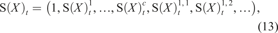
A multitude of practical data streams and time series can be regarded as a path, for example, video, sound, financial data, control signals, handwriting, etc. The path signature transforms such multivariate sequential data (which may have missing or irregularly sampled values) into an infinite-length series of real numbers that uniquely represents a trajectory through Euclidean space. Although formally distinct and with notably different properties, one useful intuition is to think of the signature of a path as akin to a Fourier transform, where paths are summarised by an infinite series of feature space coefficients. Consider a path X traversing space
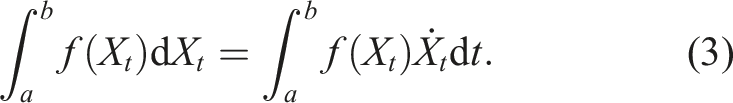
In particular, note that the mapping t → f(X
t
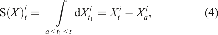
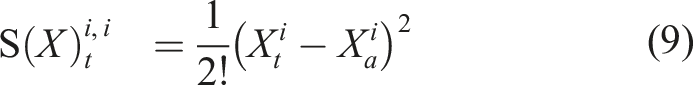
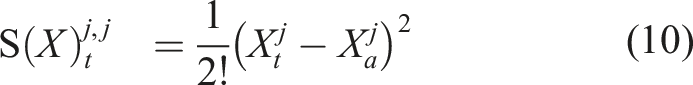
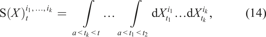
) is also a path. In fact, equation (3) is an instance of the Riemann–Stieltjes integral (Chevyrev and Kormilitzin, 2016), which computes the integral of one path against another. Let us now define the 1-fold iterated integral, which computes the increment of the ith coordinate of the path at time t as:
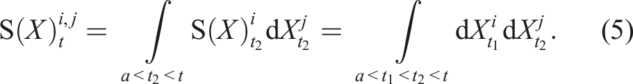
Since the 1-fold iterated integral is a path, we can apply the same iterated integral and define the 2-fold iterated integral (Chen, 1954; 1977) as: Geometric interpretation of the path signature. The path is moving from time 0 to time t. The dashed line is the chord connecting the two end-points of the path. Left and centre: These images depict two components of the 2-fold iterated integral of this path. Right: The image shows the Lévy area enclosed by the path and its chord.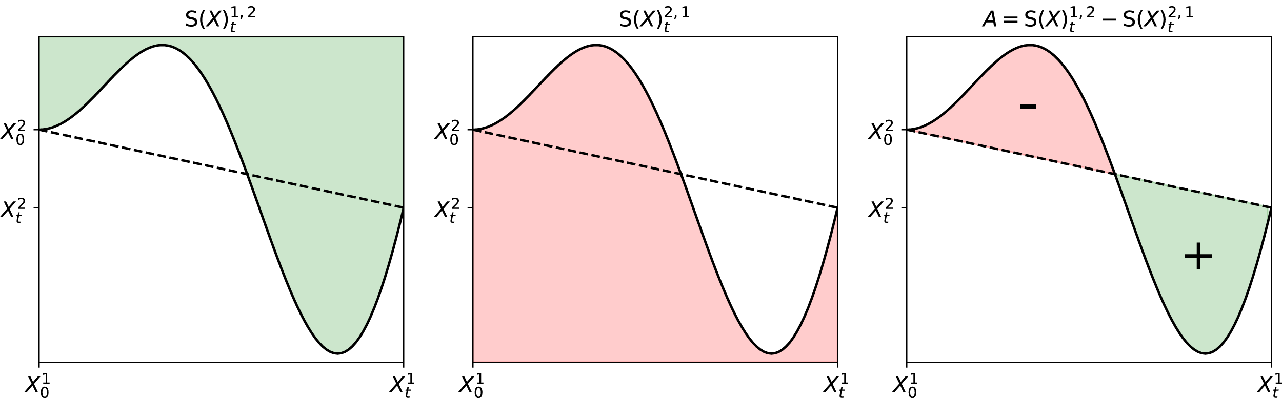


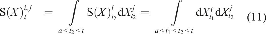
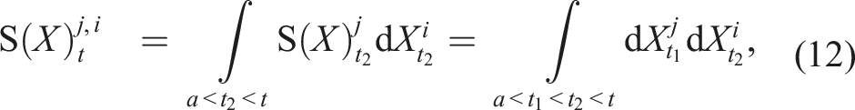
The geometric interpretation of the k-fold iterated integral for k > 2 of a two-dimensional path is not trivial and therefore not presented here. Nonetheless, by analogy, for a three-dimensional path, the 1-fold, 2-fold, and 3-fold iterated integrals are units of displacement, area, and volume, respectively. Informally, we can proceed indefinitely, and we retrieve the path signature by collecting all iterated integrals of the path X.
Signature (Chevyrev and Kormilitzin, 2016). The signature of a path In practice, we often apply a truncated signature up to a degree d, that is The path signature was originally introduced by Chen (Chen, 1958) who applied it to piecewise smooth paths, and further developed by Lyons and others (Améndola et al., 2019; Boedihardjo et al., 2016; Hambly and Lyons, 2010; Lyons, 2014). The number of elements in the path signature depends on the dimension of the input c and the degree d and is given by c
d
. Therefore, the time and space scalability of the signature is rather poor (O(c
d
)), but this can be alleviated with the use of kernel methods as we will discuss in Section 4. The signature of a path has several interesting properties, which make it inherently interesting for applications in robotics.

3.2.1. Canonical feature map for paths
For all effects, the path signature can be thought of as a linear feature map (Fermanian, 2021) that transforms multivariate sequential data into an infinite length series of real numbers, which uniquely represents a trajectory through Euclidean space. This is valid even for paths with missing or irregularly sampled values (Boedihardjo et al., 2016; Hambly and Lyons, 2010).
3.2.2. Time-reversal
We informally define the time-reversed path
3.2.3. Uniqueness
The signature of every non-tree-like path is unique (Hambly and Lyons, 2010). A tree-like path is one in which a section exactly retraces itself. Tree-like paths are quite common in real data (e.g., in cyclic actions), and this could be a limiting factor of the signature’s application. However, it has been proven (Hambly and Lyons, 2010) that if a path has at least one monotonous coordinate, then its signature is unique. The main significance of this result is that it provides a practical procedure to guarantee signature uniqueness by, for example, including a time dimension.
3.2.4. Invariance under reparametrisation
An important difficulty when vying for diversity in trajectory optimisation is the potential symmetry present in the data. This is particularly true when dealing with sequential data, such as, for instance, trajectories of an autonomous vehicle. In this case, the problem is compounded as there is an infinite group of symmetries given by the reparametrisation of a path (i.e., continuous surjections in the time domain to itself), each leading to distinct similarity metrics. In contrast, the path signature acts as a filter that is invariant to reparametrisation removing these troublesome symmetries and resulting in the same features as shown in Figure 4. Signature invariance to reparametrisation. Left: Plot of the coordinates of a two-dimensional path P
t
over time. Here, 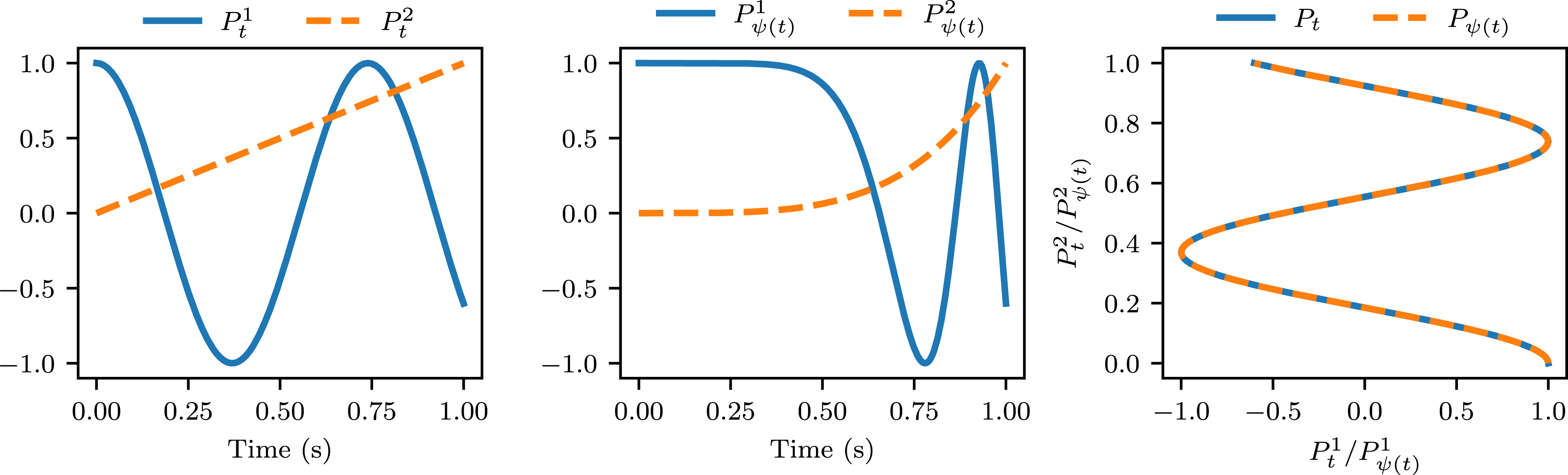
3.2.5. Dimension is independent of path length
The final property we will emphasise is how the dimension of the signature depends on its degree and the intrinsic dimension of the path but is independent of the path length. In other words, the signature dimension is invariant to the degree of discretisation of the path.
3.3. Stein variational gradient descent
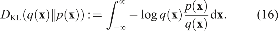
Variational inference (VI) (Blei et al., 2017) is an established and powerful method for approximating challenging posterior distributions in Bayesian Statistics. As opposed to Markov chain Monte Carlo (MCMC) (Haugh, 2021) approaches, in VI, the inference problem is cast as an optimisation problem in which a candidate distribution

The main challenge that arises is defining an appropriate


4. Method
Our main goal is to find a diverse set of solutions to the problem presented in Section 3.1. To that end, we begin by reformulating equation (1) as a probabilistic inference problem. Next, we show that we can apply SVGD to approximate the posterior distribution of trajectories with a set of sampled paths. Finally, in Section 4.3, we present our main contribution discussing how we can promote diversity among the sample paths by leveraging the Path Signature Kernel.
4.1. Stein variational motion planning
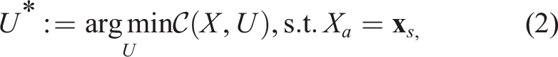
To reframe the trajectory optimisation problem described in equation (1) as probabilistic inference, we introduce a binary optimality criterion,
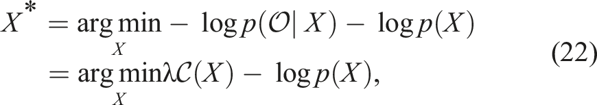
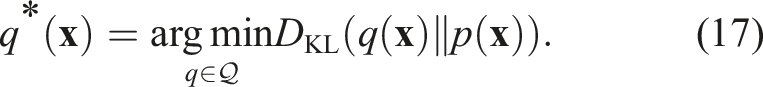
Rather than finding the MAP solution, we are interested in approximating the full posterior distribution, which may be multi-modal, and generating diverse solutions for the planning problem. As discussed in Section 3.3, we can apply SVGD to approximate the posterior distribution with a collection of particles. In the case at hand, each of such particles is a sampled path, such that equation (21) can be rewritten as:
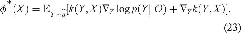
The score function presented in equation (23) is composed of two competing forces. On one hand, we have the kernel-smoothed gradient of the log-posterior pushing particles towards regions of higher probability, whereas the second term acts as a repulsive force, pushing particles away from one another.
It is worth emphasising that the kernel function is static, that is, it does not consider the sequential nature of the input paths. In effect, for a path of dimension c and s discrete time-steps, the inputs are projected onto a space
Finally, the posterior gradient can be computed by applying Bayes’ rule, resulting in:

4.2. Stein variational motion planning with smooth paths
In previous work (Barfoot et al., 2014; Dong et al., 2016; Lambert and Boots, 2021; Mukadam et al., 2018), the prior distribution in equation (24) is defined in a way to promote smoothness on generated paths. This typically revolves around defining Gaussian Processes (Rasmussen and Williams, 2006) as priors and leveraging factor graphs for efficiency. Although effective, this approach still requires several latent variables to describe a desired trajectory, which implies on a higher dimensional inference problem.
Importantly, the problem dimensionality is directly related to the amount of repulsive force exerted by the kernel. In large dimensional problems, the repulsive force of translation-invariant kernels vanishes, allowing particles to concentrate around the posterior modes, which results in an underestimation of the posterior variance (Zhuo et al., 2018). This problem is further accentuated when considering the static nature of the kernel function, as discussed in the previous section.
In order to keep the inference problem low-dimensional while still enforcing smooth paths, we make use of natural cubic splines and aim to optimise the location of a small number of knots. These knots may be initialised in different ways, such as perturbations around a linear interpolation from the starting state
Since path smoothness is induced by the splines, the choice of prior is more functionally related to the problem at hand. If one desires some degree of regularisation on the trajectory optimisation, a multivariate Gaussian prior centred at the placement of the initial knots may be used. Conversely, if we only wish to ensure the knots are within certain bounds, a less informative smoothed approximation of the uniform prior may be used. More concretely, for a box B = x: a ≤ x ≤ b, such prior would be defined as:

As discussed in Section 3.1, the cost functional
4.3. Stein variational motion planning with path signature Kernel
In this section, we present our main contribution, which is a new formulation for motion planning in which Path Signature can be used to efficiently promote diversity in trajectory optimisation through the use of Signature Kernels. In Section 3, we discussed some desirable properties of the signature transform. The key insight is that the space of linear combination of signatures forms an algebra and makes the signature a faithful feature map for trajectories (Kiraly and Oberhauser, 2019).
With that in mind, perhaps the most straightforward use of the signature would be to redefine the kernel used in equations (20) and (21) as
Hence, we take a different approach and proceed by first projecting paths to an RKHS onto which we will then compute the signature. That is, given a kernel
At first glance, this operation would further deteriorate scalability since the most useful
Nonetheless, recent work (Salvi et al., 2021) proved that for two continuously differentiable input paths, the complete signature kernel,

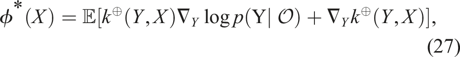
Hence, we can directly apply k⊕ in equation (23), and we now have a way to properly represent sequential data in feature space, resulting in the final gradient update function:
5. Results
In this section, we present results to demonstrate the correctness and applicability of our method in a set of simulated experiments, ranging from simple 2D motion planning to a challenging benchmark for robotic manipulators. For another introductory example, a path following task is presented in Appendix B.
5.1. Motion planning on 2D terrain
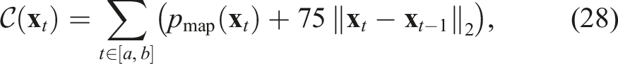
Our first set of experiments consists of trajectory optimisation in a randomised 2D terrain illustrated in Figure 2. Regions of higher cost, or hills, are shown in a darker shade, whereas valleys are in a lighter colour. The terrain is parameterised by a series of isotropic Multivariate Gaussian distributions placed randomly according to a Halton sequence and aggregated into a Gaussian Mixture Model denoted by pmap.
In this instance, paths are parameterised by natural cubic splines with N k = 2 intermediary knots, apart from the start and goal state. Note that this is a design choice and the method is agnostic to the type of parameterisation chosen to encode the paths, like, for instance, GP or Random Fourier Features (RFF). Characteristics such as smoothness, computational cost, and differentiability should be taken into account when selecting a given parameterisation.
Our goal is to find the best placement for these knots to find paths from origin to goal that avoid regions of high cost but are not too long. We adopt the following cost function in order to balance trajectory length and navigability:
The initial knots are randomly placed, and the plots in Figure 2 show the final 20 trajectories found with three different optimisation methods. Furthermore, the colour of each path depicts its normalised final cost. On the left, we can see the solutions found with Batch Gradient Descent (BGD) and note how all trajectories converge to two modes of similar cost. The SVMP results are more diverse but failed to capture one of the BGD modes. Also note how, when multiple trajectories converge to a single trough, the spline knots are pushed away by the repulsive force resulting in suboptimal solutions. On the other hand, the trajectories found by SigSVGD are not only more diverse, finding more homotopic solutions, but are also able to coexist in the narrow valleys. This is possible since the repulsive force is being computed in the signature space and not based on the placement of the knots. Furthermore, notice how, for the same reason, the paths are more direct and coordinated when compared to SVMP.
5.2. Point-mass navigation on an obstacle grid
Here, our goal is to demonstrate the benefits of applying the signature kernel Model Predictive Control (MPC). To that end, we reproduce the point-mass planar navigation task presented in Barcelos et al. (2021) and (Lambert et al. (2020) and compare SVMPC against a modified implementation using SigSVGD. The objective is to navigate a holonomic point-mass robot from start to goal through an obstacle grid. Since the system dynamics is represented as a double integrator model with non-unitary mass m, the particle acceleration is given by
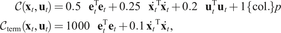
To create a controlled environment with several multi-modal solutions, obstacles are placed equidistantly in a grid (see Figure 5). The simulator performs a simple collision check based on the particle’s state and prevents any future movement in case a collision is detected, simulating a crash. Barriers are also placed at the environment boundaries to prevent the robot from easily circumventing the obstacle grid. As the indicator function makes the cost function non-differentiable, we need to compute approximate gradients using Monte Carlo sampling (Lambert et al., 2020). Furthermore, since we are using a stochastic controller, we also include CMA-ES and Model Predictive Path Integral (MPPI) (Williams et al., 2016) in the benchmark. A detailed account of the hyper-parameters used in the experiment is presented in Appendix A. Point-mass navigation trajectories. The plot shows an intermediate time-step of the navigation task for SigSVGD, on the left, and SVMPC, on the right. An inset plot enlarges a patch of the map just ahead of the point mass. The rollout colour indicates from which of the policies, that is, paths in the optimisation, they originate, whereas fixed motion primitives are shown in purple. Note how rollouts generated by SigSVGD are more dispersed, providing a better gradient for policy updates.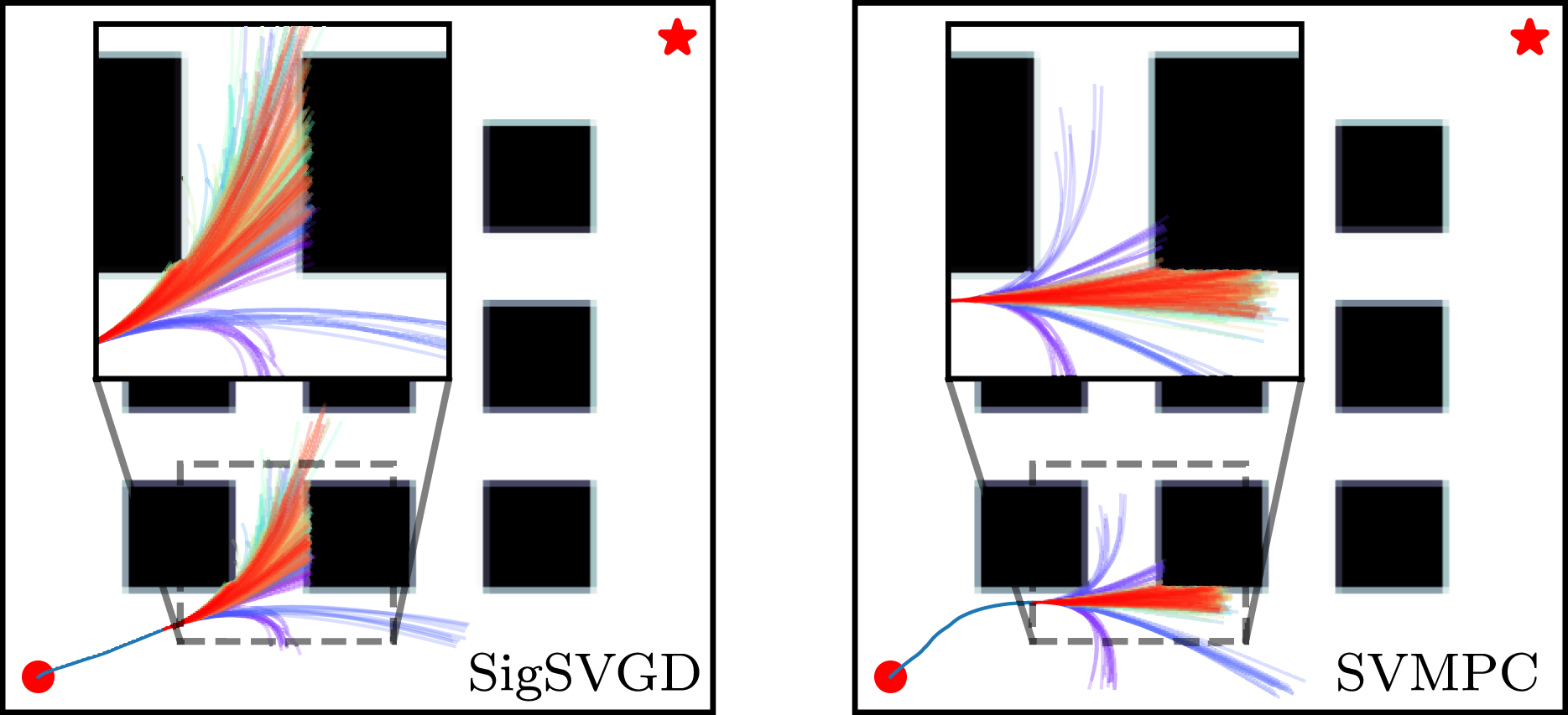
In this experiment, each of the particles in the optimisation is a path that represents the mean of a stochastic control policy. Gradients for the policy updates are generated by sampling the control policies and evaluating rollouts via an implicit model of the environment. As CMA-ES only entertains a single solution at any given time, to make the results comparable, we increase the amount of samples it evaluates at each step to be equivalent to the number of policies times the number of samples in SVMPC. One addition to the algorithm in Lambert et al. (2020) is the inclusion of particles with predefined primitive control policies which are not optimised. For example, policies which constantly apply the minimum, maximum, or no acceleration are all valid primitives. These primitive policies are also included in every candidate solution set of CMA-ES.
Point-mass navigation results.
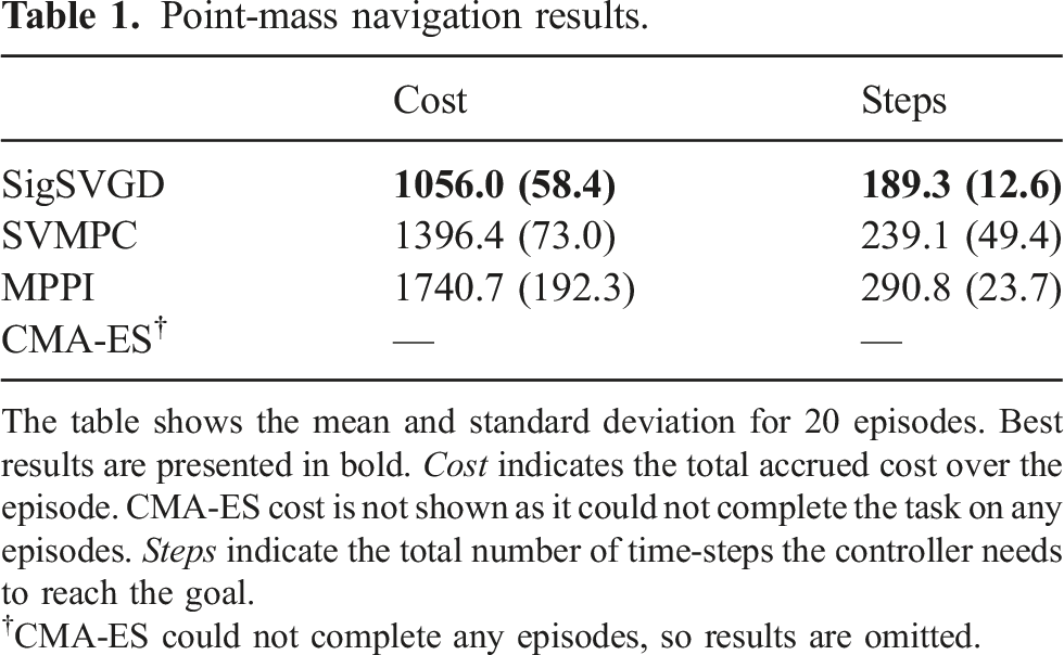
The table shows the mean and standard deviation for 20 episodes. Best results are presented in bold. Cost indicates the total accrued cost over the episode. CMA-ES cost is not shown as it could not complete the task on any episodes. Steps indicate the total number of time-steps the controller needs to reach the goal.
†CMA-ES could not complete any episodes, so results are omitted.
5.3. Benchmark comparison on robotic manipulator
To test our approach on a more complex planning problem, we compare batch gradient descent (i.e., parallel gradient descent on different initialisations), SVMP and SigSVGD in robotic manipulation problems generated using MotionBenchMaker (Chamzas et al., 2022). A problem consists of a scene with randomly placed obstacles and a consistent request to move the manipulator from its starting pose to a target configuration. For each scene in the benchmark, we generate four different requests and run the optimisation with five random seeds for a total of 20 episodes per scene. The numerical experiments are conducted on a system with Intel i7-10750H at 5.0 GHz with 12 cores CPU, 32 GB RAM (system memory) and an NVIDIA GeForce GTX 1650 Ti Mobile GPU.
The robot used is a Franka Emika Panda with 7 Degrees of Freedom (DOF). The cost function is designed to generate trajectories that are smooth, collision-free and with a short displacement of the robot’s end-effector. We once again resort to a fully-differentiable function to reduce the extraneous influence of approximating gradients with Monte Carlo samples. As is typical in motion planning, the optimisation is performed directly in configuration space (C-space), which simplifies the search for feasible plans. To reduce the sampling space and promote smooth trajectories, we once again parameterise the path of each of the robot joints with natural cubic splines, adopting three intermediary knots besides those at the initial and target poses.
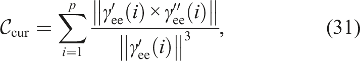
5.3.1. Regularising path length and dynamical motions
Finally, the use of splines to interpolate the trajectories ensures smoothness in generated trajectories, but that does not necessarily imply in smooth dynamics for the manipulator. To visualise this, consider, for example, a trajectory in 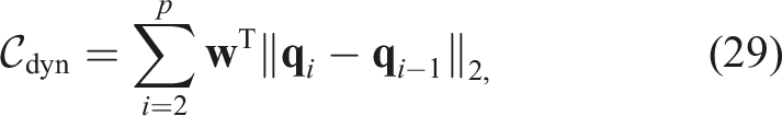
Let 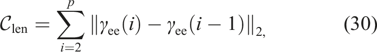

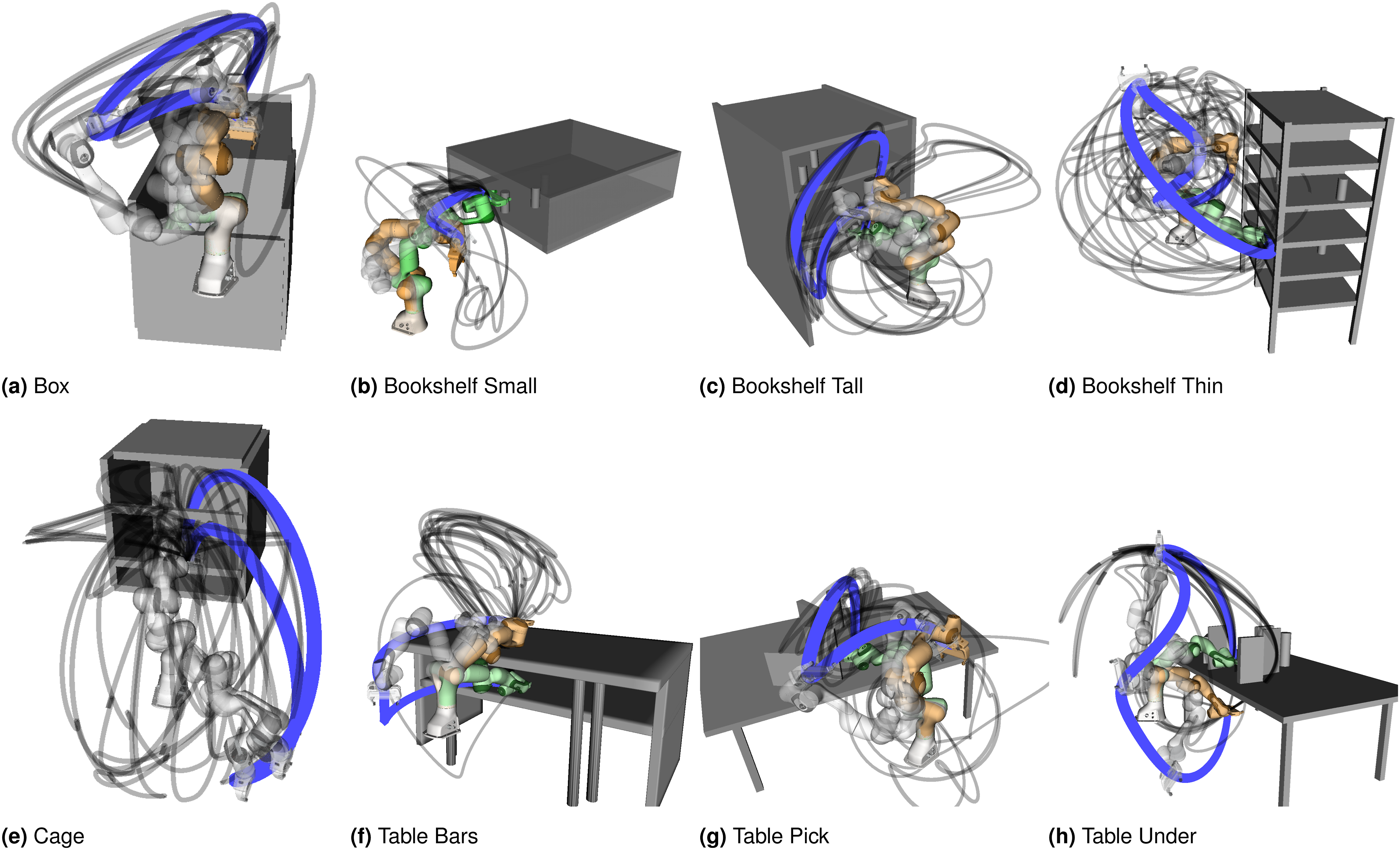
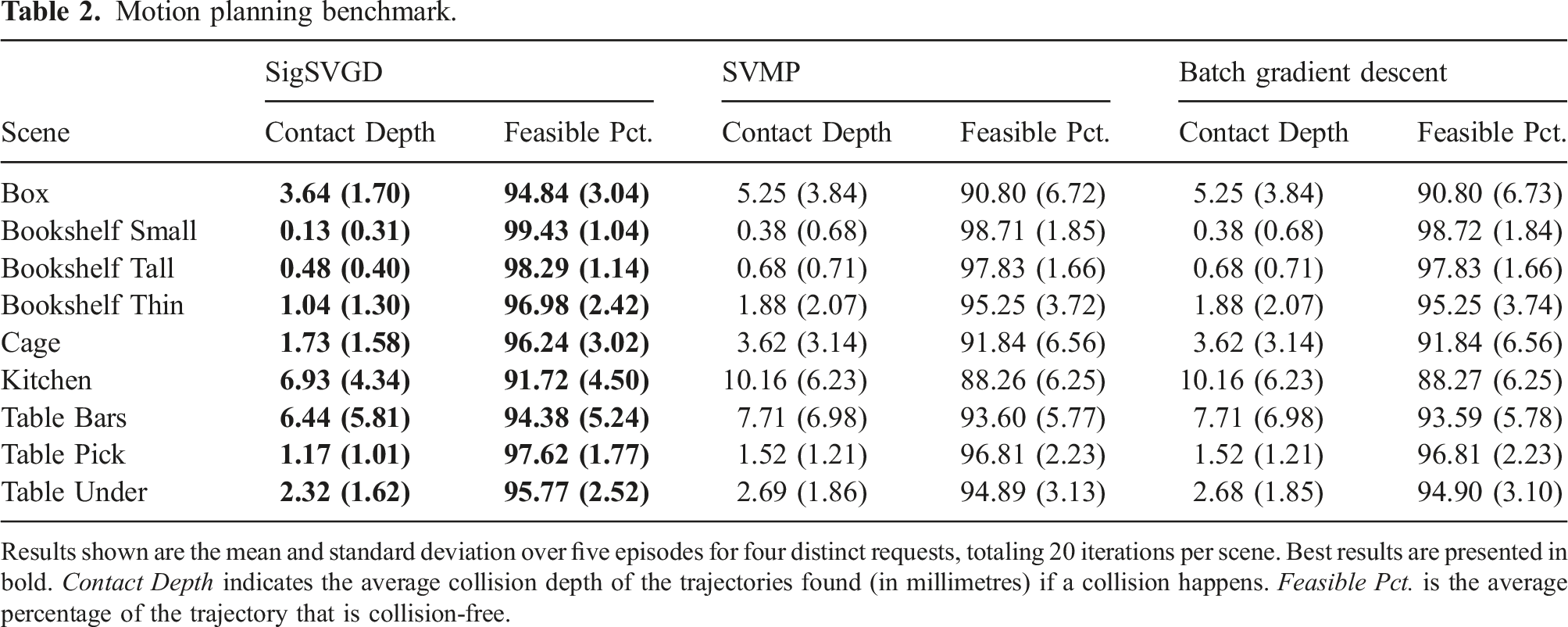
The results shown on Figure 6 demonstrate how SigSVGD achieves better results in almost all metrics for every scenario. The proper representation of paths results in better exploration of the configuration space and leads to better global properties of the solutions found. This can be seen in Figure 7, which shows the end-effector paths for SigSVGD and SVMP. One of such paths is also illustrated in Figure 1. For completeness, we have also included results for trajectory feasibility and respective contact depth on collisions. Not only did SigSVGD not compromise on feasibility, but also showed a higher percentage of feasible trajectories and lower contact depths for rollouts in collision (see Table 2). Motion planning benchmark. Results shown are the mean and standard deviation over five episodes for four distinct requests, totalling 20 iterations per scene. The best result is highlighted with a hatched bar. Lowest cost depicts the cost of the best trajectory found. Path length is the piecewise linear approximation of the end-effector trajectory length for the best trajectory. NLL indicates the negative log likelihood and, since we are using an exponential likelihood, represents the total cost of all sampled trajectories. Visualisation of SigSVGD in the motion planning benchmark. The Blue and Grey lines denote the end-effector’s trajectories with the former highlighting the trajectory with the lowest cost. The Orange and Green tinted robot poses denote the start and target configurations, respectively. The translucent robot poses denote in-between configurations of the lowest-cost solution. (a) Box. (b) Bookshelf Small. (c) Bookshelf Tall. (d) Bookshelf Thin. (e) Cage. (f) Table Bars. (g) Table Pick. (h) Table Under. Motion planning benchmark. Results shown are the mean and standard deviation over five episodes for four distinct requests, totaling 20 iterations per scene. Best results are presented in bold. Contact Depth indicates the average collision depth of the trajectories found (in millimetres) if a collision happens. Feasible Pct. is the average percentage of the trajectory that is collision-free.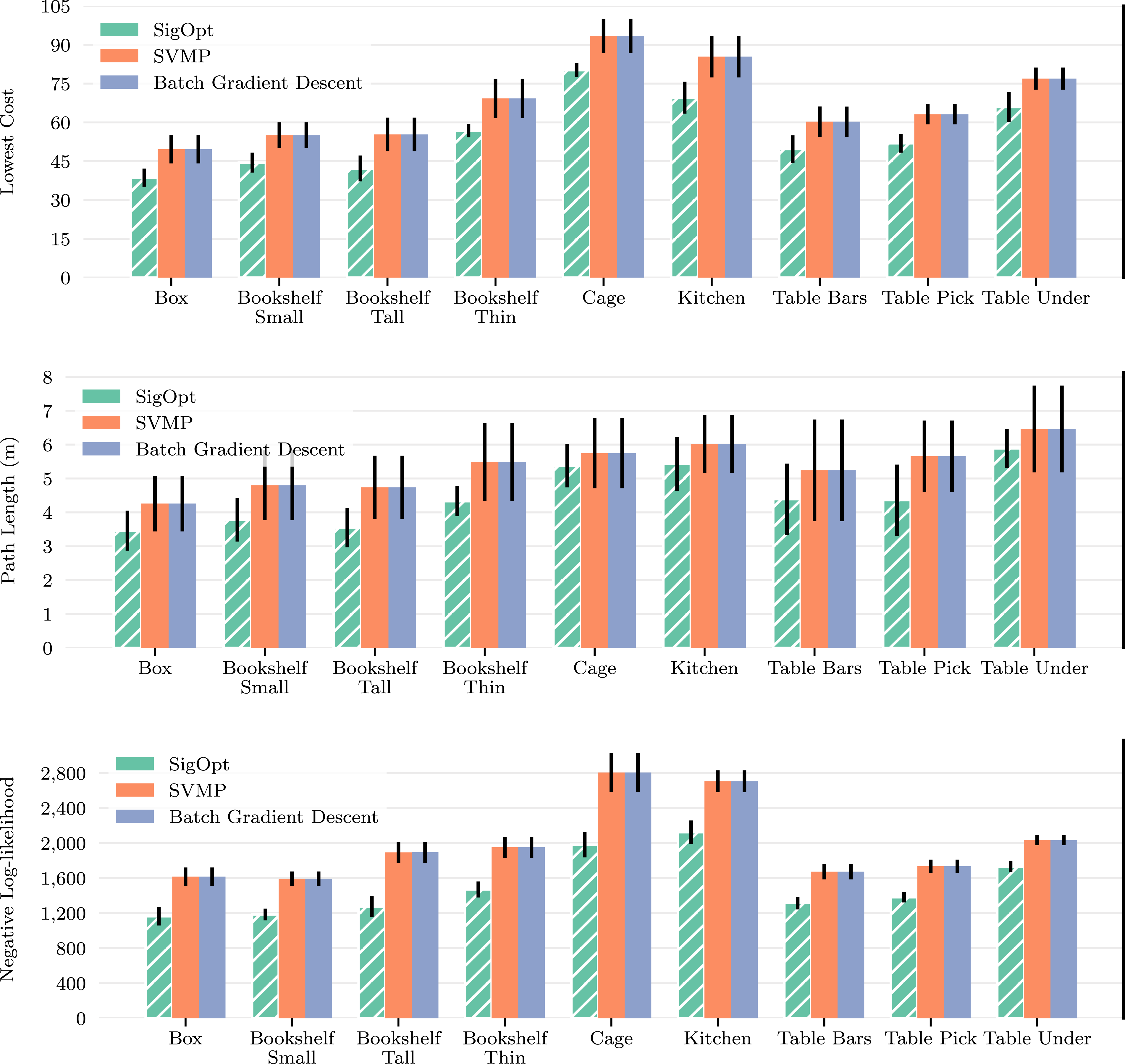
5.3.2. Robot collision as continuous cost
Typically, collision-checking is a binary check and non-differentiable. To generate differentiable collision checking with informative gradients, we resort to continuous occupancy grids. Occupancy grid maps are often generated from noisy and uncertain sensor measurement by discretising the space
In this work, we trade off the extra complexity of the methods previously mentioned for a coarser but simpler approach. Inspired by Danielczuk et al. (2021), we learn the occupancy of each scene using a neural network as a universal function approximator. We train the network to approximate a continuous function that returns the likelihood of a robot configuration being occupied. The rationale for this choice is that, since all methods are optimised under the same conditions, the comparative results should not be substantially impacted by the overall quality of the map. Additionally, the trained network is fast to query and fast to obtain derivatives with respect to inputs, properties that are beneficial for querying of large batches of coordinates for motion planning.
Given a dataset of n pairs of coordinates and a binary value which indicates whether the coordinate is occupied, that is,
A similar problem occurs when ascertaining whether a given configuration of the robot’s joints is unfeasible, leading to a self-collision. We address this issue in a similar manner by training a separate neural network to approximate a continuous function fs-col, which maps configurations of the robot to the likelihood of them being in self-collision. More precisely,
5.3.3. Bringing collision costs from workspace to configuration space
Collision checking requires information about the workspace geometry of the robot to determine whether it overlaps with objects in the environment. On the other hand, we assume that the robot movement is defined and optimised in C-space. The cost functions to shape robot behaviour are often defined in the Cartesian task space. We denote C-space as
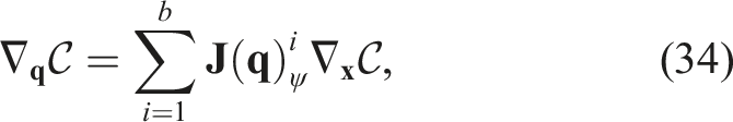
We start by defining b body points on the robot, each with a forward kinematics function ψ
i
mapping configurations to the Cartesian coordinates 
5.3.4. Combining trajectory optimisation with RRT-initialised trajectories
To further explore the applicability of SigSVGD in scenarios where initial trajectories are already in proximity to a local minimum, we conducted a modified version of the experiment illustrated in Figures 6 and 7. Instead of randomly initialising the spline knots, we apply RRT*-Connect to initialise the k-many motion planning problem, where k = 20 is the number of particles used in our experiment. Subsequently, we proceed with the batch optimisation procedure just like in the previous experiment. It is important to note that motion planning with RRT*-Connect is inherently sequential, foregoing the advantages of parallel computation and introducing a notable overhead. Nevertheless, we adopt this approach in a controlled experiment to assess the contribution of SigSVGD under these specific conditions. The results are shown in Figure 8. The outcomes for each simulation are more variegated than those of Figure 6, but illustrate how even under these new conditions, SigSVGD helps in finding a better solution in most of the simulated scenarios. Motion planning benchmark with RRT*-Connect initialisation. Results shown are the mean and standard deviation over five episodes for four distinct requests, totalling 20 iterations per scene. The best result is highlighted with a hatched bar. Lowest cost depicts the cost of the best trajectory found. Path length is the piecewise linear approximation of the end-effector trajectory length for the best trajectory. NLL indicates the negative log likelihood and, since we are using an exponential likelihood, represents the total cost of all sampled trajectories.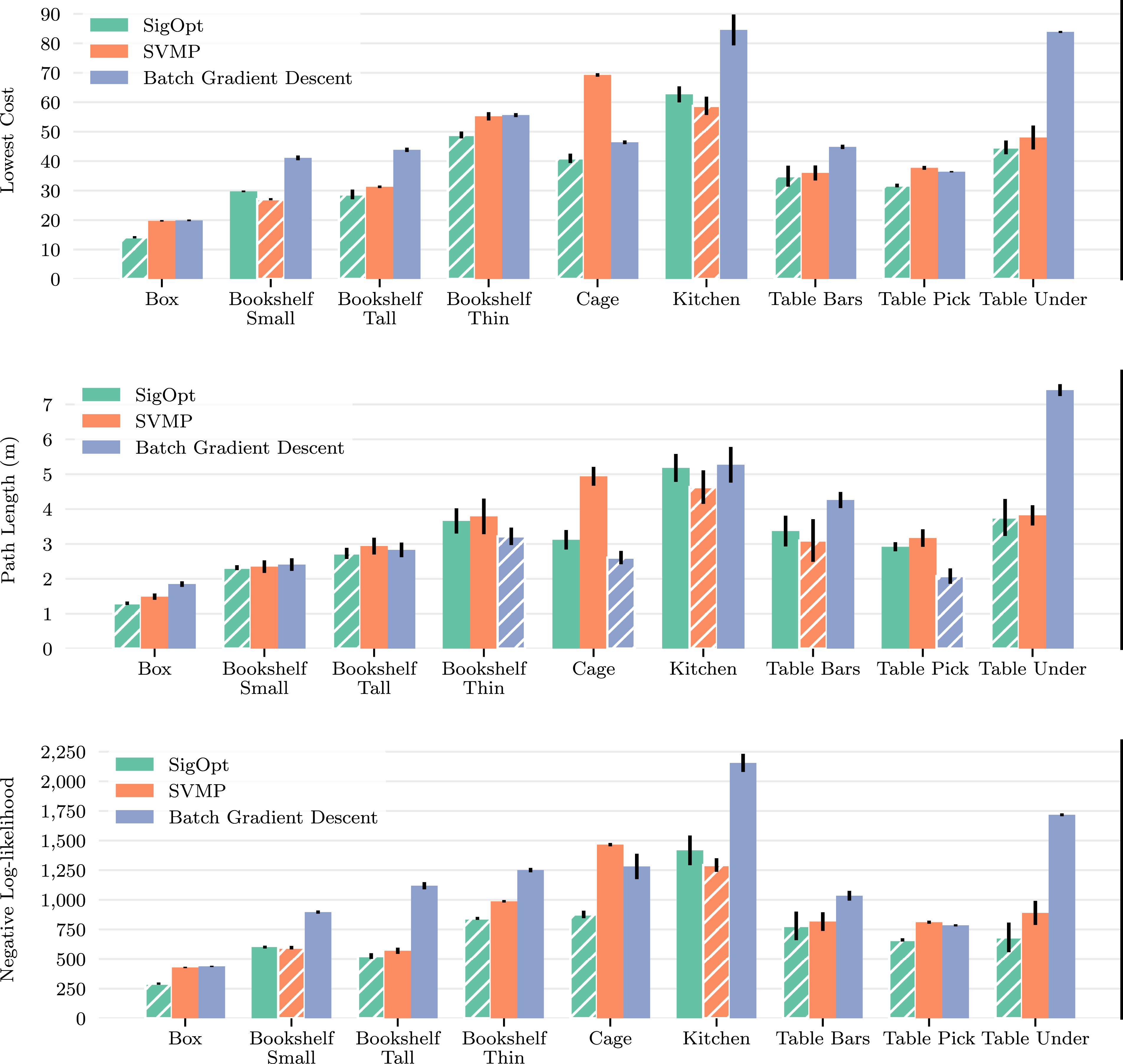
6. Conclusion
This work, to the best of our knowledge, is the first to introduce the use of path signatures for trajectory optimisation in robotics. We discuss how this transformation can be used as a canonical linear feature map to represent trajectories and how it possesses many desirable properties, such as invariance under time reparametrisation. We use these ideas to construct SigSVGD, a sequential kernel method to solve control and motion planning problems in a variational inference setting. It approximates the posterior distribution over optimal paths with an empirical distribution comprised of a set of vector-valued particles that encode the sequential nature of paths and which are all optimised in parallel.
In previous work, it has been shown that approaching the optimisation from the variational perspective alleviates the problem of local optimality, providing a more diverse set of solutions. We argue that the use of signatures improves on previous work and can lead to even better global properties. Despite the signature poor scalability, we show how we can construct fast and paralellisable signature kernels by leveraging recent results in rough path theory. The RKHS induced by this kernel creates a structured space that captures the sequential nature of paths. This is demonstrated through an extensive set of experiments that the structure provided helps the functional optimisation, leading to better global solutions than equivalent methods without it. We hope the ideas herein presented will serve an inspiration for further research and stimulate a groundswell of new work capitalising on the benefits of signatures in many other fields within the robotics community.
Footnotes
Declaration of conflicting interests
The author(s) declared no potential conflicts of interest with respect to the research, authorship, and/or publication of this article.
Funding
The author(s) received no financial support for the research, authorship, and/or publication of this article.