The INSANE dataset: Large number of sensors for challenging UAV flights in Mars analog,outdoor,and out-/indoor transition scenarios

Abstract

For real-world applications, autonomous mobile robotic platforms must be capable of navigating safely in a multitude of different and dynamic environments with accurate and robust localization being a key prerequisite. To support further research in this domain, we present the INSANE datasets (Increased Number of Sensors for developing Advanced and Novel Estimators)—a collection of versatile Micro Aerial Vehicle (MAV) datasets for cross-environment localization. The datasets provide various scenarios with multiple stages of difficulty for localization methods. These scenarios range from trajectories in the controlled environment of an indoor motion capture facility, to experiments where the vehicle performs an outdoor maneuver and transitions into a building, requiring changes of sensor modalities, up to purely outdoor flight maneuvers in a challenging Mars analog environment to simulate scenarios which current and future Mars helicopters would need to perform. The presented work aims to provide data that reflects real-world scenarios and sensor effects. The extensive sensor suite includes various sensor categories, including multiple Inertial Measurement Units (IMUs) and cameras. Sensor data is made available as unprocessed measurements and each dataset provides highly accurate ground truth, including the outdoor experiments where a dual Real-Time Kinematic (RTK) Global Navigation Satellite System (GNSS) setup provides sub-degree and centimeter accuracy (1-sigma). The sensor suite also includes a dedicated high-rate IMU to capture all the vibration dynamics of the vehicle during flight to support research on novel machine learning-based sensor signal enhancement methods for improved localization. The datasets and post-processing tools are available at: https://sst.aau.at/cns/datasets/insane-dataset/

1. Introduction

Real-world datasets are an essential part of the research and development process in the field of robotics. When developing new methods and algorithms, one of the first steps is to test and prove an approach with flawless simulated data sequences, followed by more advanced verification in which the simulated data needs to reflect real-world sensor behaviors such as noise, non-Gaussian signal distributions, and environment-based signal degradation. Modeling realistic sensor signals and their degradation linked to the environment is a difficult, if not impossible, task. At this stage, real-world datasets with accurate ground truth are a prerequisite to move from the ivory tower to real-world applications.

Existing Unmanned Aerial Vehicle (UAV) datasets focus on isolated topics such as Visual Inertial Odometry (VIO), indoor navigation, or vehicle control with aspects to energy efficiency as presented by Rodrigues et al. (2021). Datasets focusing on outdoor UAV applications are sparse, and the provided ground truth for subsequent algorithm development and evaluation is not of sufficient quality. In addition, research towards multi-environment UAV operations is progressively increasing. One example is the transition of UAVs from outdoor environments to indoor locations and vice versa. Such operations cause changes to the sensor availability, such as GNSS sensors, which become unavailable in particular phases. Other side effects include anomalies in the magnetic field, close to building structures, which affect the readings of a magnetometer, or changing light conditions affecting VIO approaches. It may also require changes of the navigation reference frames if the available sensors provide relative navigation, for example, VIO.

Autonomous tasks requiring such scenarios are package delivery applications, automated emergency response, vessel inspection (e.g., the European BugWright2 ¹ project), and long-term environmental surveying, for example, agricultural applications Malyuta et al. (2020). Corresponding research for transitioning robotic vehicles includes Congram and Barfoot (2021) and long-duration UAV autonomy with possible indoor recharging Brommer et al. (2018).

Unfortunately, openly available multi-environment data, which is necessary to elevate this field of research and to move from simulated scenarios into the real world, especially for UAVs, does not exist. Simulated environments include the work introduced by Fornasier et al. (2021) and Wang et al. (2020) as well as datasets with real sensor data but artificially augmented vision presented by Antonini et al. (2020). Yet, using simulated data for this aspect is only suitable for initial development stages as it does not account for realistic environmental effects introduced to a sensor, such as near infrastructure affecting GNSS or Ultra-Wide-Band (UWB) signals during an indoor-outdoor transition.

While the applications mentioned before require a versatile multi-sensor setup to complete a task and gain sufficient knowledge about the environment, we also want to mention the possible aspects for which this dataset can aid the development and improvement of novel multi-sensor fusion approaches. Figure 1 in the related work section shows the increased number of sensors and a wide variety of sensor modalities of the INSANE dataset compared to state-of-the-art datasets. Other UAV datasets do not carry a high number of sensors due to restricted payloads.

Figure 1.

Overview of the number of sensors and their variety categorized by the type of robotic platform for state-of-the-art datasets. Corresponding tables, which compare the individual sensor modalities in more detail, are provided in appendix A.1.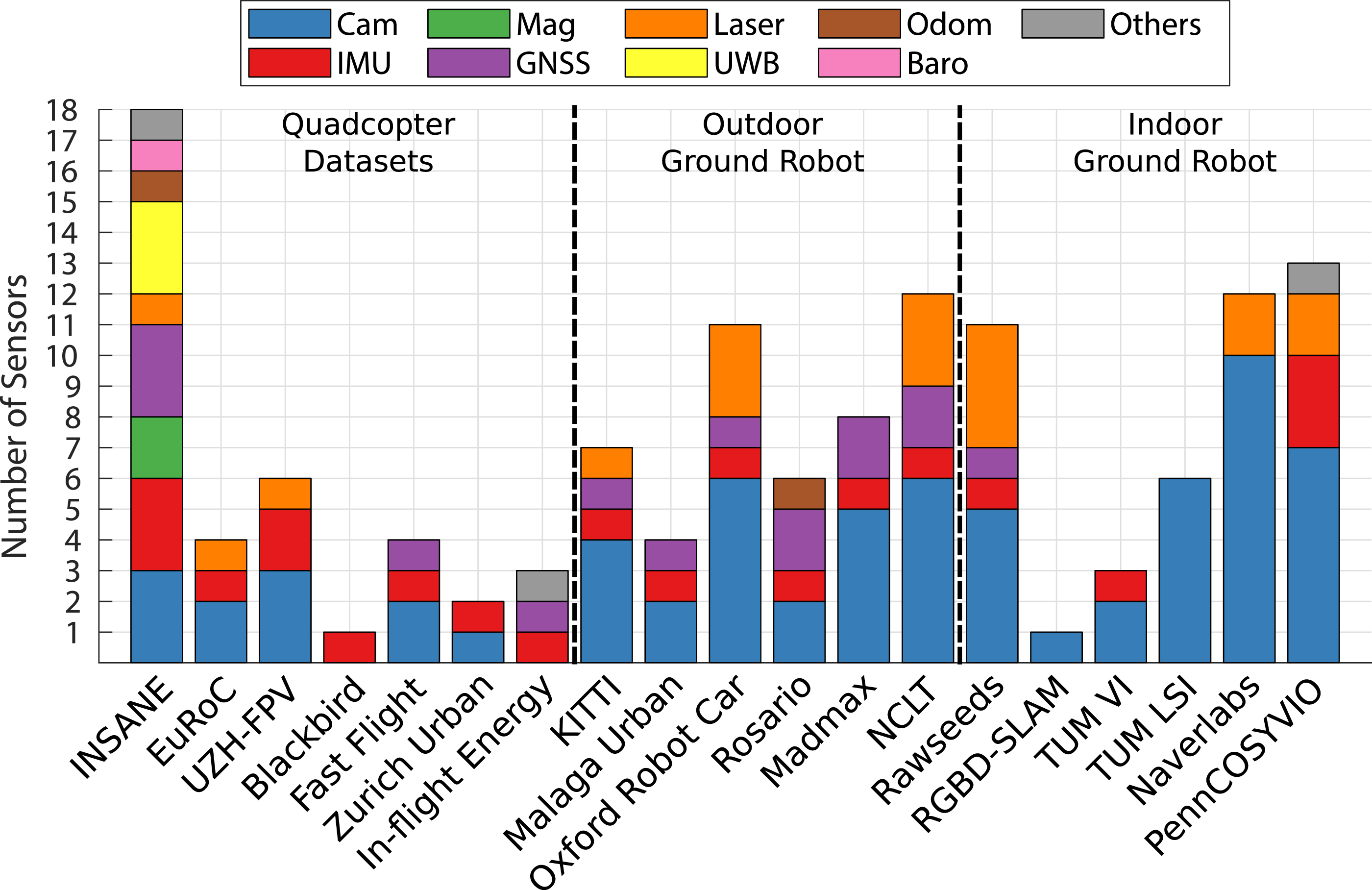

The presented INSANE flight dataset aims to overcome this limitation. With a total of 18 sensors, ranging from high-resolution navigation images over high-rate and multi-IMU signals to multi-GNSS and UWB data. This dataset provides the opportunity for the validation of localization approaches with aspects to centralized estimation and modular integration of sensor information, scalability of new methodologies, and properties to robustness and sensor switching approaches under real-world conditions. It further promotes the development for robust mapping and perception as well as the comparison of learning vs. classical approaches. Research on these topics will benefit from the increased number of sensors, the broader modality of sensor types, and the fact that this sensor data is subject to real-world sensor degradation. In addition to the variety of sensors, the dataset also focuses on scenarios for cross-environment robotics by providing a variety of cross-domain and multi-environment flight datasets with highly accurate ground truth for position and orientation (6 DoF) for indoor and outdoor setups.

For the generation of ground truth data, special attention and effort was given to the acquisition of high-quality raw (unprocessed) measurements provided by the sensors that are required to generate this ground truth. The ground truth provided for the presented dataset is given as an absolute entity and is not expressed relative to existing localization algorithms, as done by distinct related work. Thus, comparing localization algorithms to the ground truth provided by this work allows for a definite evaluation of errors without restrictions to specific metrics.

The same platform was used to record 27 datasets with accumulated trajectories of more than 2 km while operating in four distinct environmental domains. It provides the necessary data to validate individual algorithm setups in a controlled environment and gradually increases the difficulty for successive proof of algorithms and methods.

The main features are as follows:

• 6 DoF absolute ground truth with centimeter and sub-degree accuracy (1-sigma) for outdoor datasets.

• Indoor trajectories with motion capture ground truth (6 DoF millimeter and sub-degree accuracy) for the initial proof of algorithms.

• Outdoor to indoor transition trajectories with continuous absolute ground truth.

• Trajectories in a Mars analog desert environment for Mars-Helicopter analog setups, including various ground structures, cliff flight over, and cliff-wall traversing trajectories for mapping.

• Vehicle and sensor integrity, including intrinsic information such as static IMU data and Revolutions per Minute (RPM) correlated vibration data.

• Real-world sensor effects and degradation posed by individual scenarios.

• Initialization sequences for VIO algorithms.

• Inter-sensor calibrations in pre-calculated form and unprocessed calibration data sequences for custom calibration routines.

1.1. Structure

We first discuss related work and discuss differences between existing datasets in Section 2. Section 3 discusses the full system setup, outlining the properties of the vehicle in 3.1 and individual aspects of all sensors, including the general module synchronization approach in 3.2 as well as a test bench setup for a dedicated vibration test in 3.3.

Section 4 will discuss the individual environmental domains and challenges for the data that was recorded in these environments. These include simple and controlled indoor environments, more involved outdoor and outdoor/indoor transition setups at a semi-urban university location, and the Mars analog desert environment, which utilizes the full sensor suite and can be interpreted as an off-world setup and that also provides challenging VIO scenarios with ground structures that are semi-homogeneous, and terrain with high relative altitude changes. The Mars analog datasets also include high velocity, high travel distance, and higher altitude aspects. Section 5 discusses the methodology for the generation of ground truth data.

Section 6 provides a brief outline of the data structure and Section 7 shows two examples of processed data to prove the quality and usability of the data. More specifically, Section 7.1 illustrates an exemplary multi-sensor fusion scenario that requires sensor switching for an outdoor to indoor transition scenario in the semi-urban area. Section 7.2 shows a vision-only example, using VIO only with a comparison of the filter results globally aligned with ground truth for a general comparison. Sections 8 and 9 complete the paper with lessons learned and the conclusion.

2. Related work

This section provides an overview of UAV research datasets and how the presented work is positioned within this ecosystem. The majority of open-source datasets in the robotics community focus on isolated research aspects and most of them are tailored towards ground vehicles and aspects of autonomous driving. This includes large-scale outdoor datasets such as KITTI Geiger et al. (2013) (1392 × 512 images @10 Hz and IMU @10 Hz) and the Oxford dataset Maddern et al. (2017) (1280 × 960 images @16 Hz, GNSS and INS solution @50 Hz and no raw IMU data), with the later addition of sporadically sparse RTK GNSS for ground truth Maddern et al. (2020). However, given the time at which the datasets were published, the provided data rates and image resolutions are lower compared to the sensor setup of the presented work. Another ground vehicle dataset, targeted specifically for the SLAM and odometry community, is presented by Pire et al. (2019). The dataset focuses on an agricultural environment and provides stereo imagery (672 × 376 @20 Hz), IMU (140 Hz), and odometry data. The dataset uses an RTK GNSS for positional ground truth but does not provide ground truth for the global orientation.

Several indoor datasets are making use of local ground truth in the form of high-quality SLAM in post-processing. This includes the TUM-LSI large-scale indoor dataset Walch et al. (2017) and Liu et al. (2022), which adds a Leica station with fiducial markers at dedicated locations. Another dataset, for a large-scale shopping mall scenery, introduced by Naverlabs Lee et al. (2021) makes use of Structure-from-Motion (SfM) in post-processing for the generation of ground truth data. The presented work does provide data to perform the same approach if desired. However, providing post-processed SLAM/SfM data is not within the scope of this publication.

The next category of datasets concerns the indoor to outdoor transition aspect. Such datasets are mainly performed by hand-held sensor suites. Pfrommer et al. (2017) introduced the PennCOSYVIO dataset with a sensor setup that extends a Google Tango platform with additional camera modalities (2 × 752 × 480 images @20 Hz and IMU @200 Hz). The dataset features indoor and outdoor locations, but it does not make use of a GNSS sensor. The ground truth for this dataset is solely generated by utilizing pre-calibrated fiducial markers placed throughout the experiment area. Schubert et al. (2018) later introduced the TUM dataset, also using a hand-held sensor setup for indoor to outdoor trajectories without GNSS information (1024 × 1024 images @20 Hz and IMU @200 Hz). For this dataset, ground truth information is only provided for the indoor segment using a motion capture system.

Finally, datasets for the development and proof of localization algorithms for UAVs also exist, but the focus does not lie on sensor degradation and sensor switching nor cross-domain operation. The EuROC dataset introduced by Burri et al. (2016) focuses on various difficulty levels of VIO for indoor scenarios (2 × 768 × 480 images @20 Hz and IMU @200 Hz), with ground truth generated by using a motion capture system and a Leica station. The UZH-FPV drone racing dataset Delmerico et al. (2019) features dynamic flights for isolated indoor and outdoor trajectories (640 × 480 images @30 Hz and IMU @500 Hz/1000 Hz, respectively). This dataset uses a motion-capturing system for the ground truth of the indoor trajectories, and SLAM for the ground truth of the outdoor trajectories. Another interesting approach is the Blackbird dataset Antonini et al. (2020), which performs real-world flights and collects IMU (100 Hz) as well as motion capture information (360 Hz) to generate a multitude of photo-realistic vision streams, each for the same set of recorded trajectories. UAV datasets for possible future real-world applications also exist; Rodrigues et al. (2021) generated a dataset for the analysis of energy consumption for a package delivery drone. However, the dataset does not provide image streams, and the accuracy of position ground truth is only rated with ±2 m @10 Hz.

Another dataset, mainly concerning the Mars analog contribution of the presented work, is the MADMAX dataset Meyer et al. (2021). This dataset provides a sensor suite similar to the Mars-Rover but is performed in a hand-held approach. However, this dataset only provides lower rate IMU measurements (100 Hz) and lower rate image streams (1032 × 772 @15 Hz and 2064 × 1544 @4 Hz) compared to the presented INSANE dataset. This is adequate, given that a rover platform does not perform agile trajectories. The ground truth for this dataset is generated by fusing measurements from two RTK GNSS units (1 Hz) with IMU measurements, resulting in a 100 Hz filtered ground truth data stream.

Figure 1 shows a high-level overview of the number of sensors and the variety of sensor types across 19 datasets, comparing the INSANE and other datasets for quadcopters, outdoor ground robots such as cars, and indoor ground and hand-held robots. Tables 7, 8 and 9 in appendix A.1 provide an additional and very detailed comparison between these datasets.

To the best of our knowledge, no UAV dataset concerning indoor-outdoor transitioning with aspects to real-world sensor degradation and an extensive sensor suite (see Table 1) with corresponding redundancies, various frame rates and resolutions, and continuous global ground truth for outdoor, indoor, and transition areas, such as presented by this work, exists at this point.

Table 1.

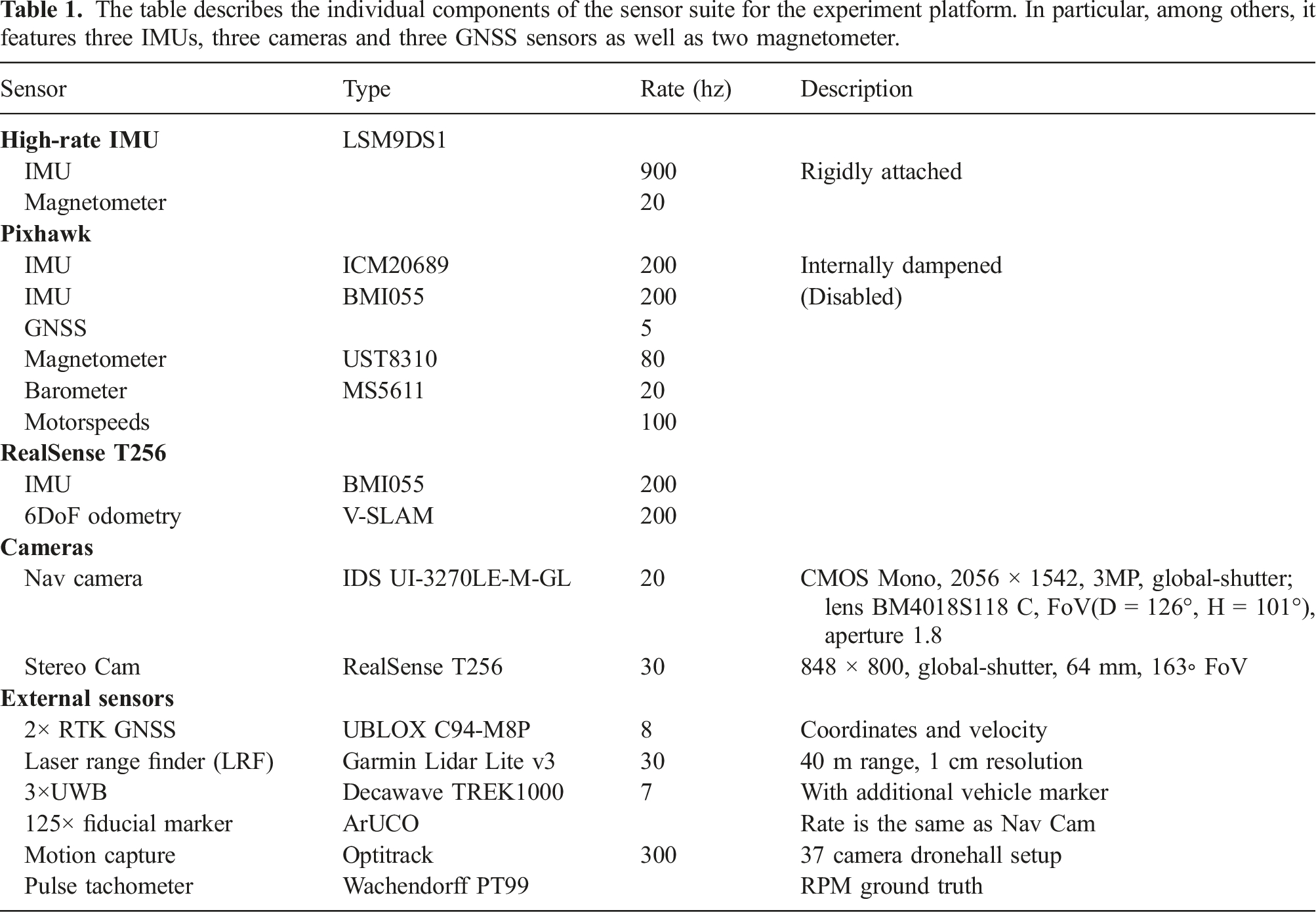
The table describes the individual components of the sensor suite for the experiment platform. In particular, among others, it features three IMUs, three cameras and three GNSS sensors as well as two magnetometer.

Sensor	Type	Rate (hz)	Description
High- rate IMU	LSM9DS1
IMU		900	Rigidly attached
Magnetometer		20
Pixhawk
IMU	ICM20689	200	Internally dampened
IMU	BMI055	200	(Disabled)
GNSS		5
Magnetometer	UST8310	80
Barometer	MS5611	20
Motorspeeds		100
RealSense T256
IMU	BMI055	200
6DoF odometry	V-SLAM	200
Cameras
Nav camera	IDS UI-3270LE-M-GL	20	CMOS Mono, 2056 × 1542, 3MP, global-shutter; lens BM4018S118 C, FoV(D = 126°, H = 101°), aperture 1.8
Stereo Cam	RealSense T256	30	848 × 800, global-shutter, 64 mm, 163◦ FoV
External sensors
2× RTK GNSS	UBLOX C94-M8P	8	Coordinates and velocity
Laser range finder (LRF)	Garmin Lidar Lite v3	30	40 m range, 1 cm resolution
3×UWB	Decawave TREK1000	7	With additional vehicle marker
125× fiducial marker	ArUCO		Rate is the same as Nav Cam
Motion capture	Optitrack	300	37 camera dronehall setup
Pulse tachometer	Wachendorff PT99		RPM ground truth

3. System setup

3.1. Vehicle configuration

All datasets have been recorded with the flight platform shown by Figure 2. The base of this platform is a commercially available carbon frame equipped with a minimal power unit, rotors, and a PixHawk4 autopilot. The base frame was heavily extended and altered from its original. The final platform setup weighs 3 kg and carries a number of additional sensors (see Table 1).

Figure 2.

This illustration shows the vehicle design with coordinate frames for the placement and orientation of the sensors on the experiment platform in (a), and the real vehicle with sensor position overlays in (b). Accurate calibration of each sensor (extrinsics and intrinsics where applicable) is given for each scenario. The method on how each sensor is calibrated and the intent on the sensor placement is described in Section 3.2.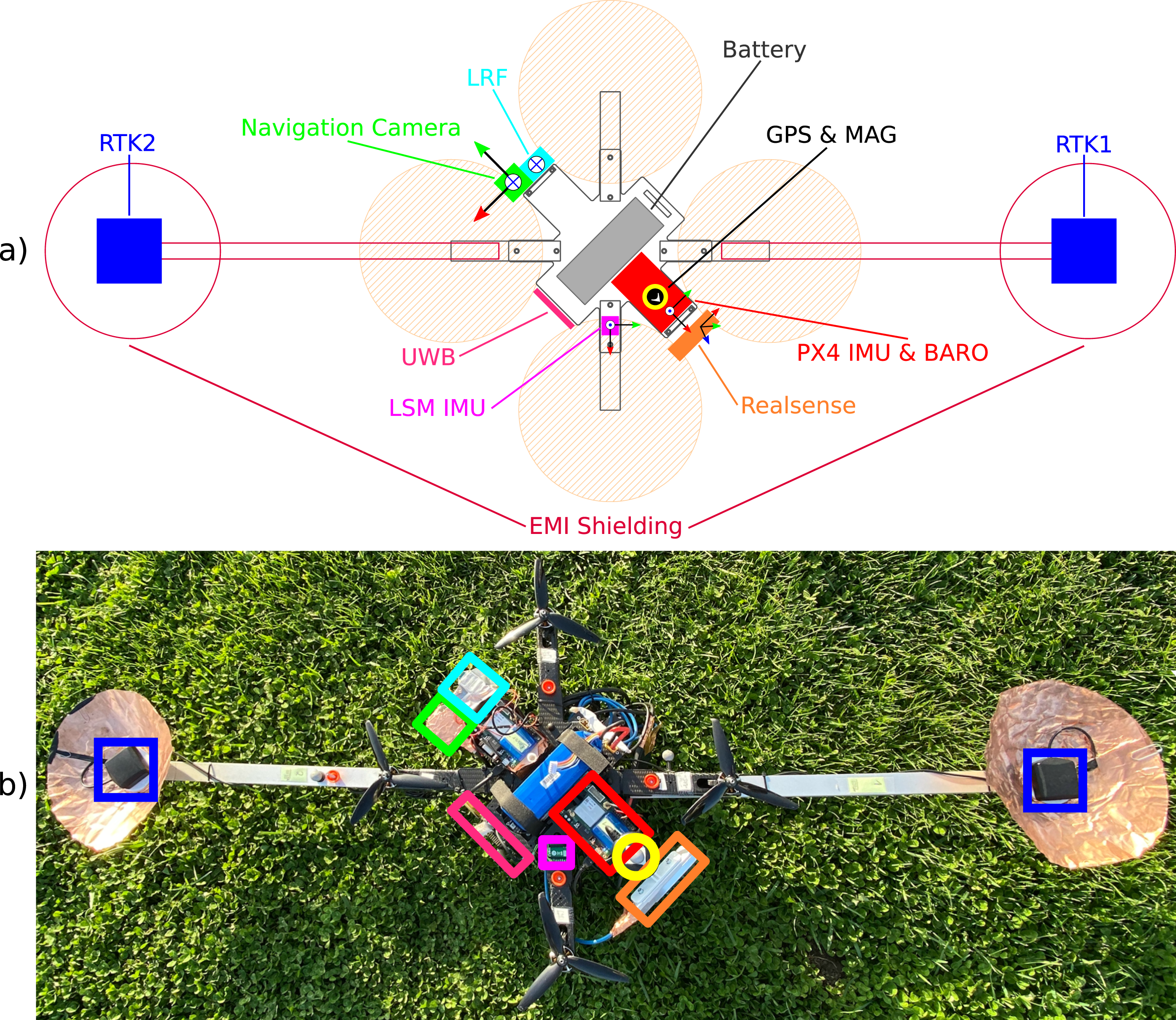

The small size of the aerial vehicle constrains the amount of additional payload. However, the UAV setup needs to be able to process the sensor data during closed-loop experiments and needs to be able to record the data of the sensor suite in raw format without loss of information. Because of this, the vehicle is equipped with two Raspberry Pi4 companion boards. This allows for computational load balancing, interface bandwidth distribution associated with a specific sensor, and distributed sensor data storage. These three aspects of the vehicle system are shown as a block diagram in Figure 3.

Figure 3.

This diagram shows the embedded companion boards and sensor integration as well as storage and interface distribution according to individual sensor data rates and the available bandwidth of the interfaces from the embedded hardware.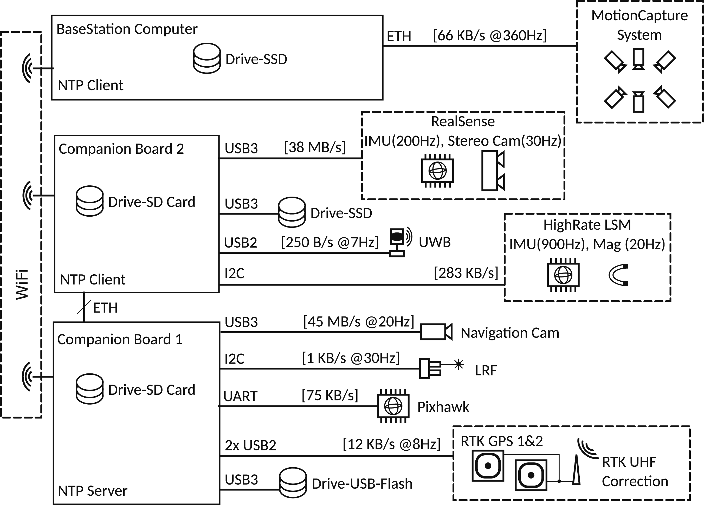

It might be of interest to the reader that the vehicle was running an in-house developed and source-available ² flight stack Scheiber et al. (2022), which is generalized and deployable across many standard computation platforms by utilizing a robust and versatile OS Stewart (2021).

The vehicle includes additional Electromagnetic Interference (EMI) shielding to allow optimal functioning of RF sensitive components such as the GNSS despite high-frequency data lines (further detailed in Section 3.2.5). Additional dust shielding and individual cooling appliances were added to the flight platform for optimal operation in the hot and sandy environment posed during the Mars analog data recording sessions.

3.2. Sensors

This section outlines the setup, calibration procedures, and individual aspects concerning the sensor suite. The sensors are summarized in Table 1.

3.2.1. IMUs

In general, the sensor suite includes four Micro-Electromechanical Systems (MEMS) IMUs. Two 200 Hz IMUs are part of the Holybro Pixhawk v5 autopilot, namely, the BMI055 from Bosch and ICM20689 from TDK. One 200 Hz BMI055 IMU is part of the RealSense T256 stereo camera, and one dedicated high-rate 900 Hz LSM9DS1 IMU from ST-Electronics is added by itself. The two IMUs of the autopilot cannot be distinguished and are actively switched based on a sensor voting scheme by default. To enable a clear association between the IMU calibration and its bias, the BMI055 IMU was deactivated. Another reason is that the RealSense T256 already provides measurements of a BMI055 type IMU. Thus, all active IMUs provided by the dataset are from individual manufacturers, providing a good range of different IMU characteristics. In addition, it may be noted that the IMUs of the autopilot are hardware dampened, shown by Figure 4 and further detailed in the vibration analysis Section 3.3 and 4.5, respectively.

Figure 4.

The sensor suite has three IMUs where each serves a different aspect. This figure shows the assembly of the primary IMU sensor within the PixHawk autopilot, on top of a damping layer that acts as a low-pass filter between the IMU and the main PCB board. This hardware filter is beneficial for closed-loop applications. However, in section 4.5, we are carrying out a vibration analysis of the vehicle. This analysis made use of the rigidly attached high-rate IMU. A brief comparison of the dampened IMU and the high-rate IMU with applied filters, designed based on the vibration analysis, is described, and the interested reader is referred to Steinbrener et al. (2022) for further use on the vibration data.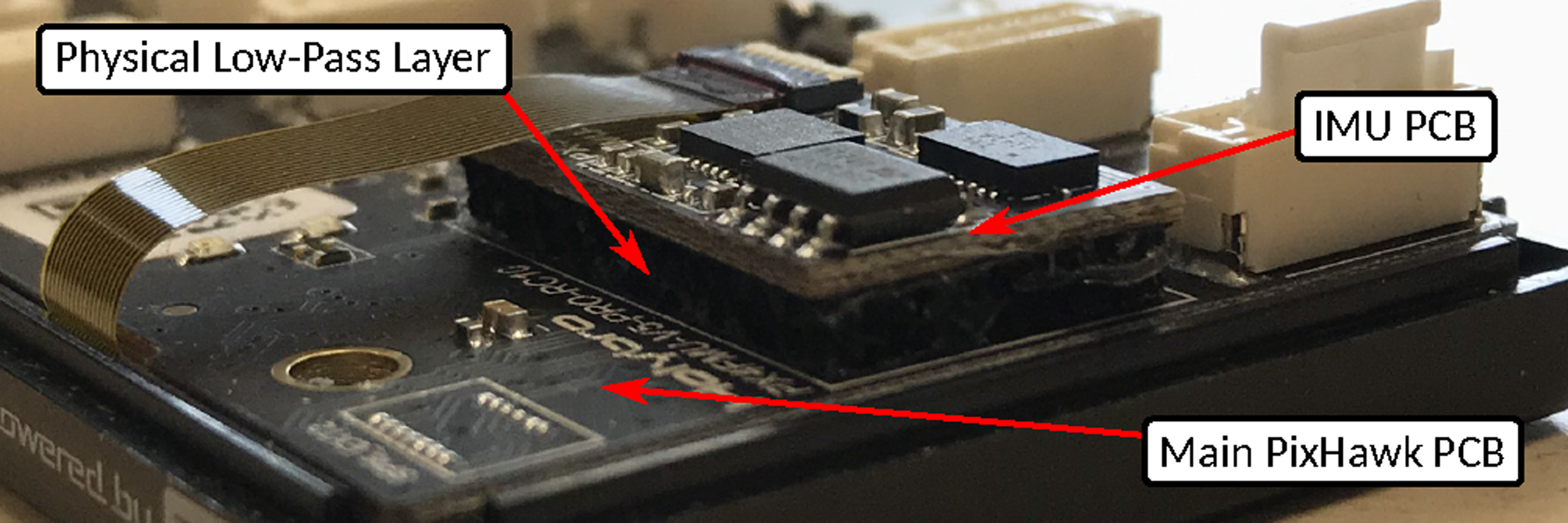

The IMU sensor positioning is shown by Figure 2. The autopilot IMU, which is referred to as the main IMU, is positioned close to the vehicle’s center, which should avoid amplified vibrations within the linear acceleration measurements.

The RealSense camera is positioned forward-facing and tilted down for ideal stereo camera positioning. Therefore, this IMU has the highest lever arm and receives the most amplification for resonances in terms of vibration. Specific scenarios also showed under-sampling effects. The measurement stream of this IMU can be seen as a challenging scenario for possible research.

The high-rate LSM9DS1 IMU is rigidly attached (not dampened) and provides measurements at more than 900 Hz to support IMU filter applications or machine learning approaches, as shown by Steinbrener et al. (2022) for active vibration analysis and noise reduction. The intrinsic calibration of the specific IMUs is done by performing the Allan variance method outlined by Freescale (2015). IMU recordings with a length of 5 hours and the corresponding tools are open-sourced with the dataset.

3.2.2. Magnetometer

The helicopter platform hosts two independent magnetometers from different manufacturers for variation in sensor characteristics and redundancy. The first module is included in the PixHawk4 sensor suite (80 Hz), and the second module is located within the external LSM9DS1 System on Chip (SoC) (20 Hz). For magnetometers, several aspects have to be considered: The intrinsic and extrinsic calibration of the sensor for its specific location on the experiment platform, the magnetic variation which depends on the geolocation, and local magnetic disturbances posed by the environment. The dataset includes a default magnetometer calibration for this vehicle and dedicated magnetometer calibration datasets, which allows for different calibration methods by the user.

It is important to note that the magnetic variation at the locations in which the dataset was recorded are not negligible. This variation depends on the geolocation and concerns the magnetic inclination (spherical elevation) and the declination (spherical azimuth), which build the local direction and strength of the magnetic field. The pertinent information is available online. ³ Location-dependent variables and descriptions for the datasets can be found in Section 4. Tables 2, 3, and 4 specifically address the magnetic variation.

Table 2.

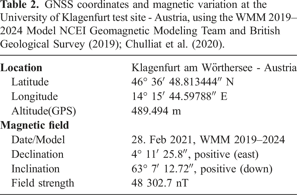
GNSS coordinates and magnetic variation at the University of Klagenfurt test site - Austria, using the WMM 2019–2024 Model NCEI Geomagnetic Modeling Team and British Geological Survey (2019); Chulliat et al. (2020).

Location	Klagenfurt am Wörthersee - Austria
Latitude	46° 36′ 48.813444″ N
Longitude	14° 15′ 44.59788″ E
Altitude(GPS)	489.494 m
Magnetic field
Date/Model	28. Feb 2021, WMM 2019–2024
Declination	4° 11′ 25.8″, positive (east)
Inclination	63° 7′ 12.72″, positive (down)
Field strength	48 302.7 nT

Table 3.

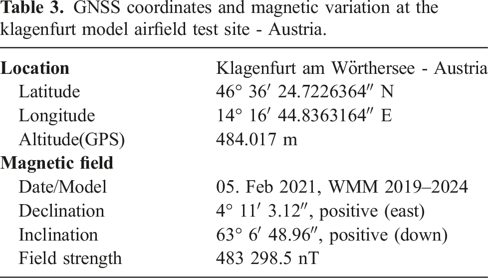
GNSS coordinates and magnetic variation at the klagenfurt model airfield test site - Austria.

Location	Klagenfurt am Wörthersee - Austria
Latitude	46° 36′ 24.7226364″ N
Longitude	14° 16′ 44.8363164″ E
Altitude(GPS)	484.017 m
Magnetic field
Date/Model	05. Feb 2021, WMM 2019–2024
Declination	4° 11′ 3.12″, positive (east)
Inclination	63° 6′ 48.96″, positive (down)
Field strength	483 298.5 nT

Table 4.

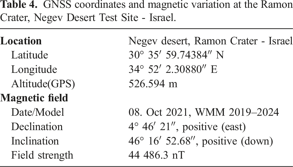
GNSS coordinates and magnetic variation at the Ramon Crater, Negev Desert Test Site - Israel.

Location	Negev desert, Ramon Crater - Israel
Latitude	30° 35′ 59.74384″ N
Longitude	34° 52′ 2.30880″ E
Altitude(GPS)	526.594 m
Magnetic field
Date/Model	08. Oct 2021, WMM 2019–2024
Declination	4° 46′ 21″, positive (east)
Inclination	46° 16′ 52.68″, positive (down)
Field strength	44 486.3 nT

The provided data segments can be used to calculate the intrinsic and extrinsic calibration of a magnetometer with respect to an IMU sensor. The intrinsic calibration of a magnetometer concerns hard-/and soft-iron effects. Both effects are mainly dependent on the mounting location of the sensor. Hard-iron effects cause a fixed offset in the magnetometer readings, while soft-iron effects affect the magnetic field strength and its direction locally. As shown by Figure 5, the red sphere shows raw magnetic measurements, and the blue sphere shows measurements that are compensated for their hard- and soft-iron effects. The red sphere is not only shifted off-center due to hard-iron effects but also distorted in its spherical shape due to the mentioned soft-iron effects.

Figure 5.

The image illustrates the offset for the magnetometer measurements from the PX4 platform, as an example on the magnetometer intrinsic calibration for hard- and soft-iron effects. The calibration is provided for all magnetometers.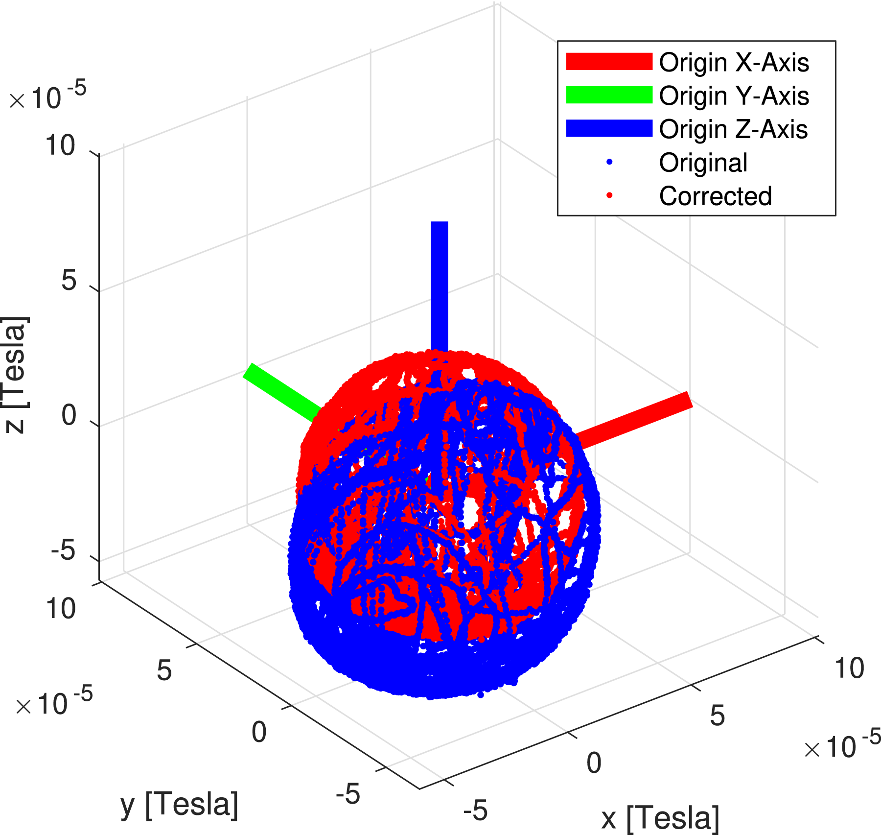

The calibration data was recorded in a non-occluded environment, and the vehicle was rotated around various rotational axes such that the magnetic vector, if projected onto a sphere, covers this sphere sufficiently. At first, an ellipsoid fit for the raw data was performed and the center of mass for this ellipsoid was found. This provides the general offset of the ellipsoid ${\mathbf{b}}_{\text{ct}}\in {\mathbb{R}}^{3\times 3}$ . Afterward, a transformation was found which transforms the ellipsoid into a sphere ${\mathbf{t}}_{\text{sp}}\in {\mathbb{R}}^{3\times 3}$ . Knowing both parameters, individual magnetometer measurements can be corrected by applying ${\mathbf{m}}_{\text{corr}}={\mathbf{t}}_{\text{sp}}\left({\mathbf{m}}_{\text{raw}}-{\mathbf{b}}_{\text{ct}}\right)$ . Detailed information on this method can be found in Vasconcelos et al. (2011).

After finding the intrinsic calibration, the extrinsic calibration between the IMU and magnetometer as well as the local magnetic inclination can be found. This is done by applying the method outlined in Papafotis and Sotiriadis (2020). Individual data sequences were recorded which provide static rotations of the vehicle in all six rotational directions with respect to the gravity vector. This data is processed with the cost function described in Papafotis and Sotiriadis (2020) to find the most accurate rotation between the gravity and magnetic vectors, including the magnetic inclination. The dataset is published with a default calibration for the vehicle setup and with a set of tools to recompute the calibration with potentially different parameters.

The data sequences for the transition experiments show an additional, real-world effect that we aimed to capture with our dataset. Because the indoor area and surrounding elements have metal structures, the magnetic field also changes depending on the location within the environment. Figure 20 shows how the magnetic field changes when entering the indoor area. One possible approach on interacting with changes in the magnetic field is outlined in Brommer et al. (2020), which describe a method of detecting magnetic field changes with subsequent adaptation to the changing magnetic field without measurement rejection.

The magnetometer measurements for all flight sequences are not compensated nor calibrated. This provides the possibility to include online self-calibration of magnetometer intrinsics, if desired.

3.2.3. Cameras

The sensor suite includes a RealSense T256 stereo camera (848 × 800 @30 Hz) and an IDS UI-3270LE-M-GL global-shutter 3MP navigation camera (2056 × 1542 @20 Hz). The navigation camera is facing downward and is aligned with a Laser Range Finder (LRF) for associated pixel range information (see Section 3.2.4). The stereo camera faces in flight direction and is tilted by 60° towards the ground. The reason for this is threefold. First, the stereo camera observes the horizon, and horizon detection can be used to improve attitude estimation. Second, the forward-facing image stream, especially for the desert datasets, can be used to observe and map crater walls. A similar task might be included in future Mars explorations. And third, starting at the height of 2 m, the stereo camera and the navigation camera have an overlapping field of view, which allows for additional feature matching, as shown by Figure 6.

Figure 6.

Example image of the outdoor dataset, showing the overlapping FoV of the forward-down-facing stereo camera (a) and the downward-facing navigation camera (b). Labels 1–3 show the same locations in the environment. 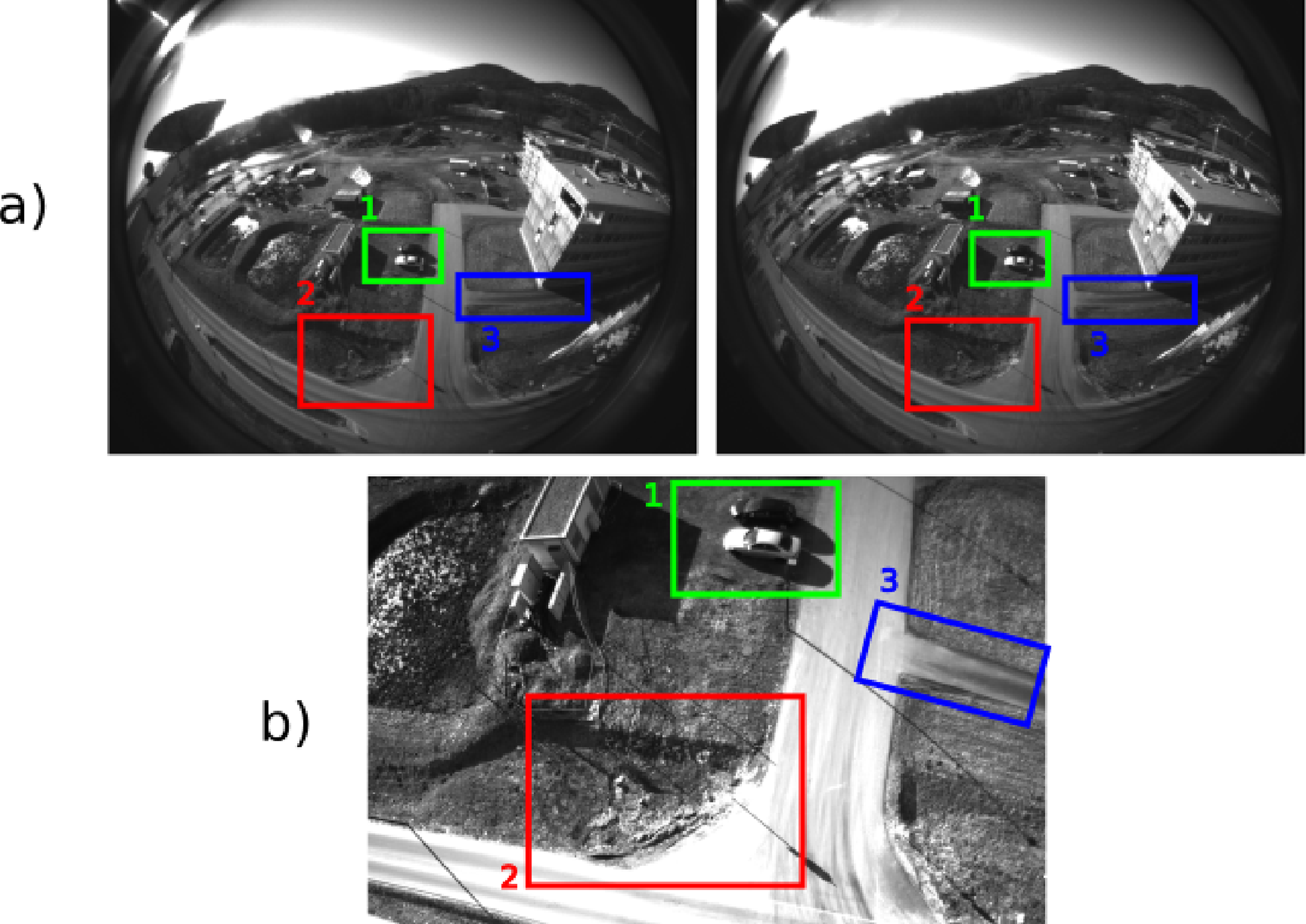Note: The image of the navigation camera is rotated by −90° and cropped to the region of interest.

Camera exposure time and gain were chosen such that motion blur is minimized. For the navigation camera, the exposure time was limited to $<5\hspace{0.17em}\text{ms}$ , and the gain was automatically adapted within a range that provides balanced brightness throughout an individual trajectory. This especially concerns the transition datasets, which have three lighting conditions: Outdoor with natural light and radiant sun, the transition area with shadow casting and reflecting snow patches, and the indoor area with artificial light providing yet another light intensity. The pure outdoor datasets, including the desert segments, make use of the same settings to reduce gain where flat patches of reflecting areas might raise the brightness of the image over a suitable threshold. The camera settings for the stereo camera are left to default values, which provide suitable imagery throughout all scenarios.

The timestamps of the navigation camera are provided by an internal clock of the camera, which is synchronized to the host system on startup. Thus, the timestamps reflect the time at which the image was taken by the camera module.

The dataset further provides dedicated recordings for the calibration of both cameras. This includes measurement streams of all IMUs and an image stream for the dedicated camera observing a checker/fiducial marker board. This data can be used to generate the intrinsic and extrinsic calibration of the cameras with respect to any IMU by using the Kalibr tool Rehder et al. (2016).

3.2.4. Laser range finder

All datasets feature a 30 Hz data stream of a Gamin Lidar Lite v3, which is a laser-based range measurement sensor. This sensor provides distance to ground measurements at a resolution of 1 cm with 2.5 cm standard deviation and operates at a distance of up to 40 m, according to the manufacturer’s description. It was noticed throughout the recording of the datasets that this sensor provides sporadic zero measurements beginning at distances of 25–30 m depending on the properties of the ground surface. The detection and rejection of these measurements is thus straightforward.

This sensor is co-mounted with the high-resolution navigation camera to provide the same setup which is used by the Mars-Helicopter Ingenuity Bayard et al. (2019). The LRF is mounted facing down in the same direction as the navigation camera (see Figure 7) to provide distance-to-ground measurements for a known pixel cluster within the navigation image.

Figure 7.

This illustration shows the co-mounted camera and laser range finder setup, which provides the same sensor setup as for the Mars-Helicopter ingenuity described by Grip et al. (2019).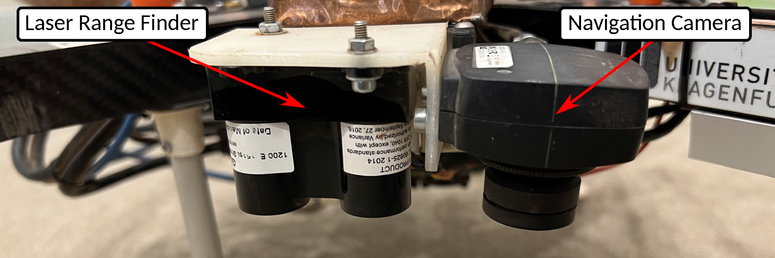

The dataset provides two options for the calibration of the rotation between the camera and the LRF. The calibration routine for the first option provides an image stream with a visible checker/fiducial target board for pose tracking and associated LRF and IMU measurements. The dataset contains measurements while the system was excited in all dimensions. A calibration can be performed with the Kalibr tool Rehder et al. (2016).

The second option is to use the data for the static setup in which the camera and the LRF are facing a wall at a defined distance. With the help of an indicator card, the spot in which the infrared LRF laser hits the wall is made visible and can thus be marked in the image and associated with a pixel location. A calibration that was generated with the second method is provided with the dataset.

3.2.5. Real-time kinematic GNSS

The sensor suite includes two off-the-shelf UBLOX C94-M8P RTK GNSS development boards with standard ceramic patch antennas. An RTK GNSS system requires a static base station that communicates corrections to the GNSS modules mounted on the vehicle. This results in highly accurate GNSS measurements with an accuracy of 1 cm to 16 cm standard deviation. For the available datasets, the threshold for the calibration of the RTK base station was set to 0.5 m.

The UBLOX C94-M8P module provides an Ultra High Frequency (UHF) module for the communication between the base station and the receivers on the vehicle. This communication channel was replaced by ZigBee modules for an extended range and reliability of the presented setup.

An RTK GNSS module has different modes of operation, which indicate the level of accuracy in position. The three primary modes are non-RTK standard GNSS, RTK float, and RTK fixed mode. Non-RTK represents the standard GNSS information without additional corrections. The RTK-float state signalizes that no unique solution for the current constellation exists. This state still benefits from RTK corrections and provides measurements with 10 cm to 16 cm accuracy. The RTK fix is the most accurate state and provides an accuracy of below 1 cm. The receiver’s status depends on a multitude of factors, such as the number of satellites, the time each satellite was tracked, and the SNR posed by the environment.

The majority of the recorded datasets provide measurements with RTK fix measurements. However, certain conditions can cause sporadic RTK-float states. The GNSS receivers also provide an estimate for the measurement covariance for significantly more detail on the measurement accuracy. This information is also provided with each dataset. We used the binary information of fixed and float RTK states for the detection of EMI issues.

As illustrated by Figure 2, the two GNSS antennas are placed on aluminum rods with a distance of 1.2 m, centered at the midpoint of the vehicle and rotated by 45° with respect to the front of the vehicle represented by the positive x-axis of the main IMU. The reason for the large baseline between the GNSS antennas is that the GNSS measurements are used for the position and rotational ground truth. Given the setup shown by Figure 8, an accuracy of η = 1 cm for one antenna, and the baseline of B = 1.2 m, the rotational error in the worst case is ϵ = 0.95°. The method used for ground truth generation is detailed in Section 5.

Figure 8.

Rotational dual GNSS error ϵ based on measurement accuracy η and the antenna baseline (b).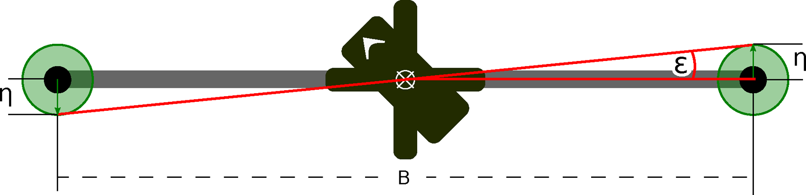

We want to briefly address the topic of EMI because the vehicle carries numerous components such as processors, RF communication, and DC/DC power converters which pose the potential for EMI with the off-the-shelf GNSS antennas: EMI in the context of high-frequency communication channels such as Bluetooth and especially USB3 has been discussed and analyzed in the literature Lin et al. (2014). Because the GNSS ceramic patch antennas for this system are standard consumer-grade products, the antennas do not make use of additional active interference rejection and provide no dedicated shielding against EMI. Initial GNSS quality tests showed impaired signal quality mainly due to the low SNR of individual satellite signals. This is caused by the onboard electronics, such as the non-shielded computation boards, sensors, and high-frequency data lines hosted by the platform. Thus, the antennas required significant additional shielding (see Figure 2) to reach an SNR, which allows the operation with high accuracy.

Different shielding designs, made from copper sheets and constructed by hand, as shown by Figure 9 have been tested. In all tests, shielding variation a) showed the most improvement for the SNR. Option c) mainly failed due to possible ground reflections of vehicle-centered EMI sources. Option b) showed good static results, but tests showed that long-term tracking of satellite signals was interrupted during rotational movement. The RTK receiver requires observations of satellite signals over more extended periods of time. Shielding option b), however, causes a barrier of signals to one side of the hemisphere, which changes based on the rotation of the vehicle. Thus, shielding variation a) was ultimately used for all data recordings. In addition to the apparent antenna shielding, the final setup required individual shielding of USB3 connection points and additional USB3 inline low-pass filter ⁴ as well as shielding and partial enclosure of computational platforms and the GNSS receivers.

Figure 9.

Tested EMI preventive variations for dedicated RTK Antenna shielding to archive sub-centimeter position accuracy and subsequent orientation accuracy for the ground truth method described in Section 5.2. (a) upward-opening with 45° side and base shielding, (b) similar to (a) but antenna and shielding tilted 40° in the vertical plane, (c) fully vertical shielding, no ground encapsulation besides antenna ground plane.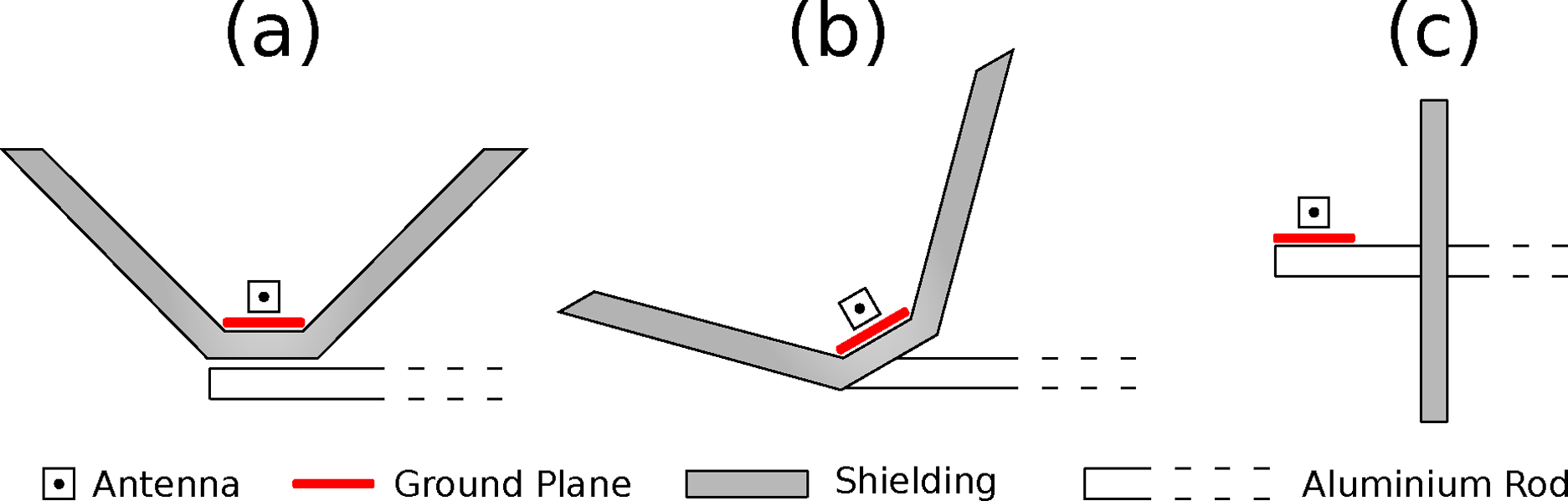

As mentioned in the previous section, the quality of the GNSS also depends on the environment. The transition data was recorded in a semi-urban environment prone to multi-path effects and a higher noise floor. On the contrary, the Mars analog datasets recorded in the Negev desert have a very low noise floor. Such circumstances can be observed in the corresponding covariances of the GNSS measurements. However, we made sure that the data in the datasets always have high-quality GNSS measurements and thus highly accurate ground truth.

3.2.6. Fiducial marker

The transition and indoor datasets provide fiducial marker landmarks. The primary purpose of these markers is to provide ground truth pose information in the transition area. When moving from outdoors to indoors, the transition area poses the challenge in which highly accurate GNSS position measurements degrade in terms of accuracy as the vehicle moves closer towards the building. At the same time, the motion capture system does not detect the vehicle yet. Thus, a field of 108 fiducial markers on eight rigid platforms is used to generate ground truth information for this trajectory segment. Each marker is a uniquely identifiable ArUco marker ⁵ generated with the library introduced in Garrido-Jurado et al. (2016). The markers become visible while the GNSS accuracy is still sufficient. During a handover phase, the GNSS and marker pose information is aligned to provide a common ground truth reference frame. After this handover phase, only the marker poses are used to generate ground truth information until the vehicle reaches the inside of the building and the area that is covered by the motion capture system. This represents the second handover phase in which a transition from marker ground truth to the motion-capturing system is performed.

The system uses two board types, five narrow-field and three wide-field marker boards. The difference between these boards is the marker size. The wide-field boards carry a 50 cm marker which becomes visible at the height of $<10\hspace{0.17em}\mathrm{m}$ . These boards are used for the outdoor area. The narrow-field boards feature smaller markers to cover lower-altitude detections during the indoor transition phase.

The fiducial marker field is calibrated based on a dedicated recording with the navigation camera, which covers all markers across boards. Marker poses T_{cam_marker} are expressed with respect to the navigation camera frame. First, all transformations between visible markers in each image ${\mathbf{T}}_{ij}={\mathbf{T}}_{\text{cam}\_i}^{-1}\hspace{0.17em}{\mathbf{T}}_{\text{cam}\_j}\hspace{0.17em}\text{with}\hspace{0.17em}\mathrm{j}<\mathrm{i}\in \mathbb{N}$ are extracted. This condition is applied to reduce complexity. Once all images have been analyzed, the individual transformations T _ij are filtered for outliers not laying within 1σ standard deviation, and the mean is generated.

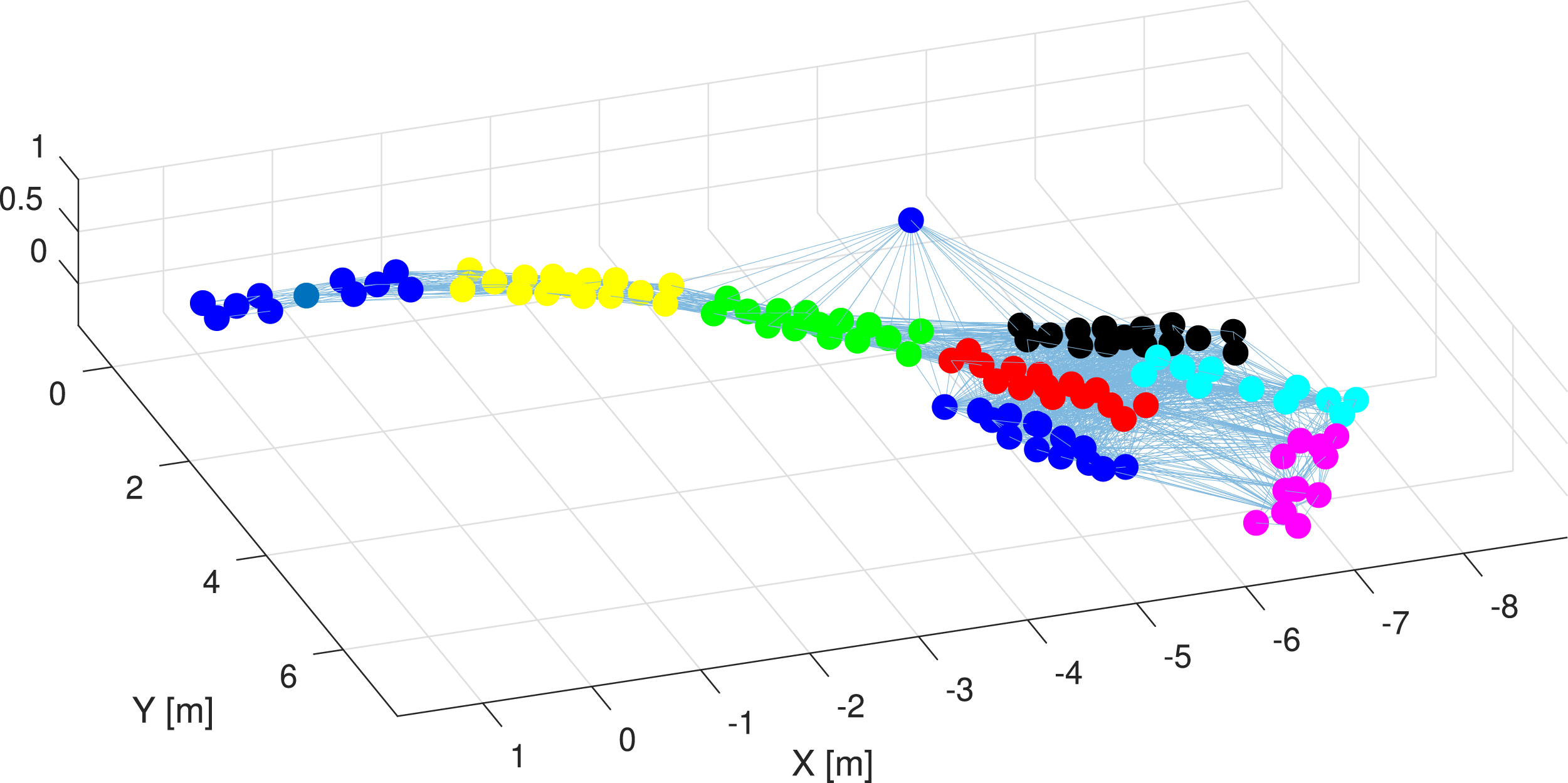
A main marker is defined, which builds the reference frame for all other markers. All individual calibrations, which may not be observed together with the main marker, are built by forming a graph search with the shortest path regarding the number of needed translations between the main marker and individual markers. Since this can include erroneous translations, the pose of each marker with respect to the main marker is improved by building multiple randomized paths between the main and individual markers, which are then averaged using the geometric median. Finally, each marker is referenced to the main marker. The board which is carrying the main marker is associated to a motion-capturing object. Thus, all markers can be expressed with respect to the motion capture system. This static calibration (visualized by Figure 11) is used to generate poses for the vehicle in the transition scenario case.

The dedicated layout for this location is shown by Figure 10 and the location of the markers after calibration is shown by Figure 11. A second purpose for these boards is the reference of UWB modules located outside the building and mounted to the marker boards. The UWB modules are placed on three boards and known locations for UWB anchor calibration.

Figure 10.

ArUco fiducial marker field design for the outdoor-indoor transition area at the Dronehall Klagenfurt. Small markers on the edge of each board provide higher accuracy for board-to-board calibration. Indoor markers are small to medium-sized due to the close proximity of the vehicle during the experiment. The outdoor marker boards carry markers that allow reliable detection up to 10 m altitude. This Setup ensures sufficient overlay in which high RTK GNSS quality is given, and the navigation camera can detect the marker. The image further shows the motion capture coverage and the placement of the UWB modules.

Figure 11.

The graph shows the placement of individual fiducial markers and their respective carrier boards in the outdoor/indoor transition area after the calibration routine. Colored dots represent individual markers detected, a dedicated color is used for each carrier board, and the lines connecting the dots represent observed relative translations between markers during the calibration procedure. The designed layout is shown in Figure 10.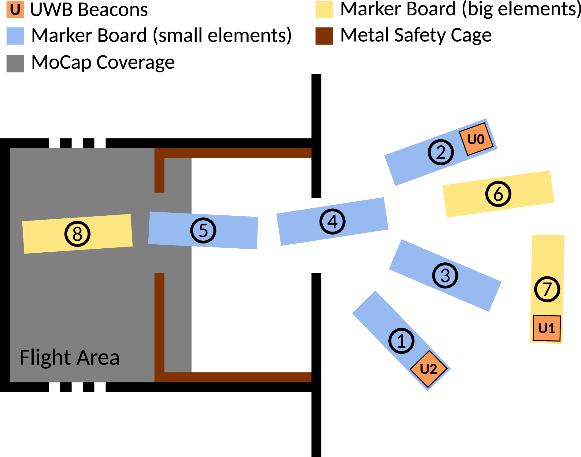

Markers can also be used as a visual aid and are present for the indoor recordings for this purpose as well. Prepared camera relative poses are provided with the datasets as well as the marker calibrations. All tools to export this data from raw data streams are open-sourced with the dataset.

3.2.7. Ultra-wideband modules

The indoor and transition datasets also feature UWB measurements. In the case of the transition dataset, the UWB modules are placed close to the building entrance and can be used for position estimates in the area in which the GNSS signals are degrading. For this purpose, the vehicle is carrying a main anchor, and three additional UWB anchors are placed on the ground. The UWB positions are shown in Figures 10 and 12. Each UWB measurement is associated with a tag.

Figure 12.

The entrance of the Dronehall, which the aerial vehicle is flying through for the recording of the transition phase datasets. The image illustrates the setup of the marker boards and the distribution of UWB modules.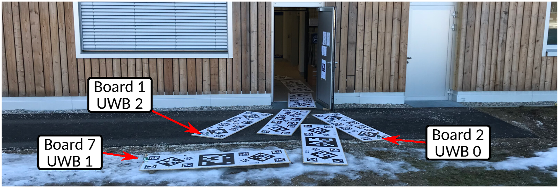

The position of the ground UWB anchors is determined by known positions on the fiducial marker boards, which can be related to the indoor motion-capturing system (see Section 3.2.6). The range in which the UWB modules provide measurements depends on environmental occlusions. While the vehicle is in the air, the first measurements are received from a distance of 30 m. A reliable stream of measurements is available at a range of $<15\hspace{0.17em}\mathrm{m}$ between UWB anchors. This includes partial areas of the indoor area.

3.2.8. Computation module time synchronization

The system diagram in Figure 3 shows that the vehicle uses two onboard computational modules for the acquisition of sensor data. These two modules are used for all experiments. A third computational instance is dedicated for the recording of motion capture data and is present for all experiments that involve the indoor area. Because multiple modules are used, inter-module time synchronization is essential to ensure coherent data association of isolated modules.

All platforms run an NTP server through Chrony, ⁶ which is set up to synchronize the system clocks at a higher rate compared to default settings. The NTP time server/reference is set up to be on module 1 of the vehicle companion boards. Module 2 and the motion capture system run an NTP client, which is continuously synchronizing to the reference time source.

We performed a dedicated test for the validation and evaluation of the quality for the time synchronization. This test was performed by utilizing the General Purpose Input/Outputs (GPIOs) of the two onboard modules, which were setup to generate a digital signal with rising edges at the same time, based on the system clock. The signal of both modules was observed with an oscilloscope. This experiment setup showed that the synchronization of the system time is accurate to 100 µs (see Figure 13) using an NTP server with continuous synchronization steps.

Figure 13.

Validation of the time synchronization for the onboard computation modules.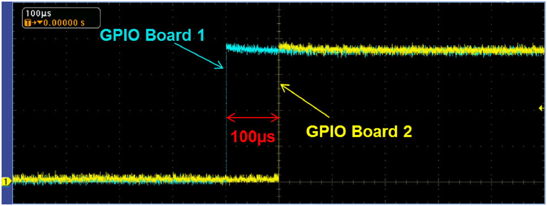

In addition to the synchronization of the computation modules, we also want to address the synchronization of the IMUs and the RealSense T256 module. The synchronization of the PX4 IMU is done software-based. The PX4 autopilot continuously synchronizes its internal clock with the computation module (host) using an NTP-like protocol for the correction of its internal clock. Timestamps of all PX4 sensor readings are then done onboard the PX4 and sent to the host with the corresponding system time.

The LSM9DS1 IMU is a single stand-alone chip which is readout via I²C. This device does not have an internal clock that can be synchronized. Thus, the timestamp generation of the LSM9DS1 is done as follows. The driver requests a measurement which triggers the acquisition of the IMU readings. The driver is immediately triggered as soon as an IMU reading was received on the I²C bus. The time difference between the request and the response is called the round trip time and is used to compensate for the communication delay, which allows for a more accurate timestamp $t_{\text{stamp}}=t_{\text{request}}+0.5\hspace{0.17em}\left(t_{\text{response}}-t_{\text{request}}\right)$ .

The synchronization of the RealSense T256, according to its documentation, ⁷ is done as follows. The T256 uses a continuous synchronization method, which provides an accuracy of 1 ms between the internal timestamps of the T256 and the host. Timestamps of the IMU data and the camera images are based on the common internal clock of the T256 and provided as the hosts system clock time.

Overall, please note that the individual sensors are not hardware synchronized. A software synchronization with an accuracy of 100 µs provides a sufficient base for sensor synchronization. We want to point out that hardware synchronization is generally not standard practice and not always possible. Novel approaches should thus not rely on synchronously triggered sensor information and allow for online estimation of delays.

However, accurate ground truth for the state of a vehicle is important for a dataset, and we perform additional synchronization for the sensors that are used to generate ground truth information in post-processing (see Section 5.3). The post-processing tools for the synchronization of the ground truth sensors are publicly available and can be used for the synchronization of other elements.

3.3. Vibration test bench

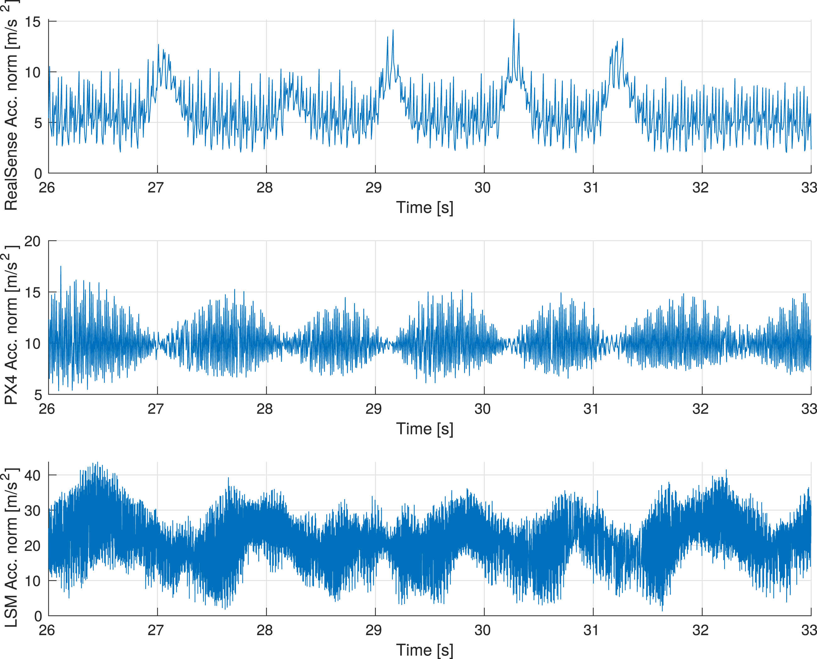
The dataset also provides additional data for vehicle-specific vibration analysis. This data is especially interesting for advanced IMU pre-filtering. The high-frequent vibration characteristics of the vehicle showed under-sampling effects for the low-rate IMUs (RealSense and PX4 @200 Hz). The RealSense is also mounted off-center, which increases this effect. Further investigation also showed that the IMU of the PX4 autopilot was hardware dampened (see Figure 4). To capture all vibration dynamics of the vehicle without hardware dampening and at a high enough sampling rate, a dedicated rigidly attached high-rate 900 Hz IMU was added to the sensor suite. Figure 15 shows a signal comparison between all IMUs. Please note that the Figure shows the norm of the linear acceleration per IMU, the change in magnitude for the LSM9DS1 IMU can be explained by the lever arm. The change in magnitude for the RealSense IMU can be caused by the lever arm as well as hardware dampening and settings from the manufacturer, which could not be changed to RAW.

The resulting dataset is suitable for an in-depth analysis of conditional sensor signal characteristics, and enables the development of adaptive noise canceling and other IMU pre-filtering techniques for improved trajectory tracking.

Data for the vibration analysis was recorded with the test bench shown in Figure 14. The flight platform was restrained by 10 ropes, eight ropes to restrain the vehicle in the vertical axis, and two ropes to further restrain rotations in the horizontal plane. The goal was to provide a semi-rigid constraint that prevents large movement of the platform but allows the nominal vibration characteristics of the vehicle that it exhibits during unconstrained, real-world flight.

Figure 14.

The image shows the vibration test bench to which the vehicle is semi-rigidly attached. Variations of static RPM and RPM sweeps of the engines provide a baseline for the vibration characteristics of the vehicle for subsequent analysis of the three IMU signals in nominal condition.

Figure 15.

This plot shows a comparison for the norm of the linear acceleration signal from the BMI055 RealSense IMU (top), the ICM20689 PX4 IMU (middle), and the LSM9DS1 IMU (bottom). The vehicle was suspended in the test bench shown by Figure 14, and the motor speeds were set to 15500 RPM. The RealSense IMU was mounted off-center and thus with a lever arm, and the PX4 IMU was mounted in the center of the vehicle. Both IMUs have a measurement rate of 200 Hz and show under-sampling effects with corresponding correlations. The LSM9DS1 IMU was also mounted off-center but has a measurement rate of 900 Hz, which results in a more accurate sampling of the vibration signals.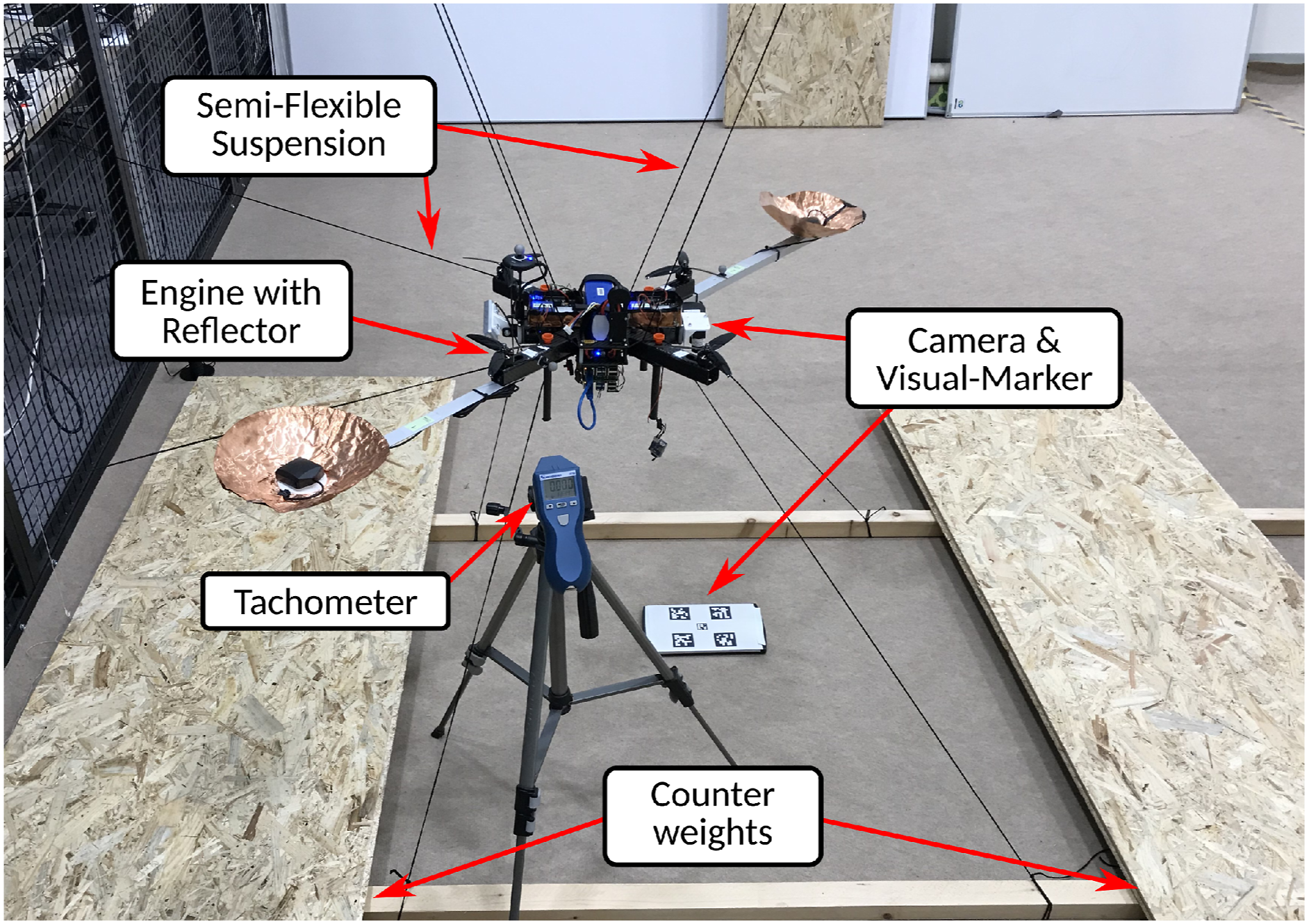

The recorded data for this scenario includes the three IMU data streams, magnetometer, pressure, downward-facing LRF, and nominal motor speeds. The PX4 firmware was adapted to stream the nominal RPM values reported by the internal mixer module. A tachometer, with provides the direct RPM of a single-engine, is used to scale the nominal motor speeds reported by the autopilot. In addition, the video streams of both cameras are recorded as well. The downward-facing navigation camera records a small five-element fiducial marker board, and the forward-tilted stereo camera observes another fiducial marker board. The pose information of the marker throughout the vibration data sequences can be used to refactor the vehicle pose data and exclude low-frequent movement—if desired. It further serves the purpose of verifying the credibility of the camera sensor mounting design.

The vibration data is recorded in nine segments with motor speeds ranging from 10% to 100% of the full nominal motor speeds. The vehicle is static before each sequence, and the motors are at a full stop before and after each segment is recorded. All four engines receive the same thrust signal through software commands, which ensures fixed and equal RPMs for all motors during the recorded sequence. A more detailed analysis of the vibration data is presented in Section 4.5.

4. Environments and experiment data

The dataset provides experiment data for three different environments. This includes the environmental transition scenario at the campus at the University of Klagenfurt, a solely outdoor setup at a model airfield, and an outdoor Mars analog setup at the Ramon crater in the Negev desert of Israel. All experiments are performed with the same vehicle setup. However, external sensor sources vary depending on the environment.

4.1. University of Klagenfurt

The location at the University of Klagenfurt is used for two types of experiments. First, the previously mentioned indoor datasets in a controlled environment for the initial tests of algorithms with the flight platform. This scenario makes use of the “Dronehall,” a motion capture environment with an area of 150 m² and 10 m in height. This area features 37 cameras and provides millimeter and sub-degree accuracy. Experiments in this environment also provide fiducial markers on the ground, visible by the navigation camera, and three UWB modules placed at different heights. Light conditions for these experiments are constant. The second type of experiment is the outdoor to indoor transition scenario. These experiments make use of the surrounding outdoor area and the indoor area of the Dronehall. This experiment also made use of fiducial marker and UWB modules but in a different configuration compared to the indoor experiments. The environmental information which applies to both experiments is summarized by Table 2.

4.1.1. Motion capture - Indoor

The indoor datasets cover three patterns at moderate speed: An upward spiral movement, a square trajectory, and a pick-and-place scenario in which the vehicle moves to multiple locations and performs a touch-down and takeoff maneuver. The three patterns are visualized by Figure 16. The pick and place scenarios have impulses in linear acceleration during the touch-down segments. The pick and place scenario also features UWB measurements for triangulation.

Figure 16.

Indoor motion capture flight patterns. 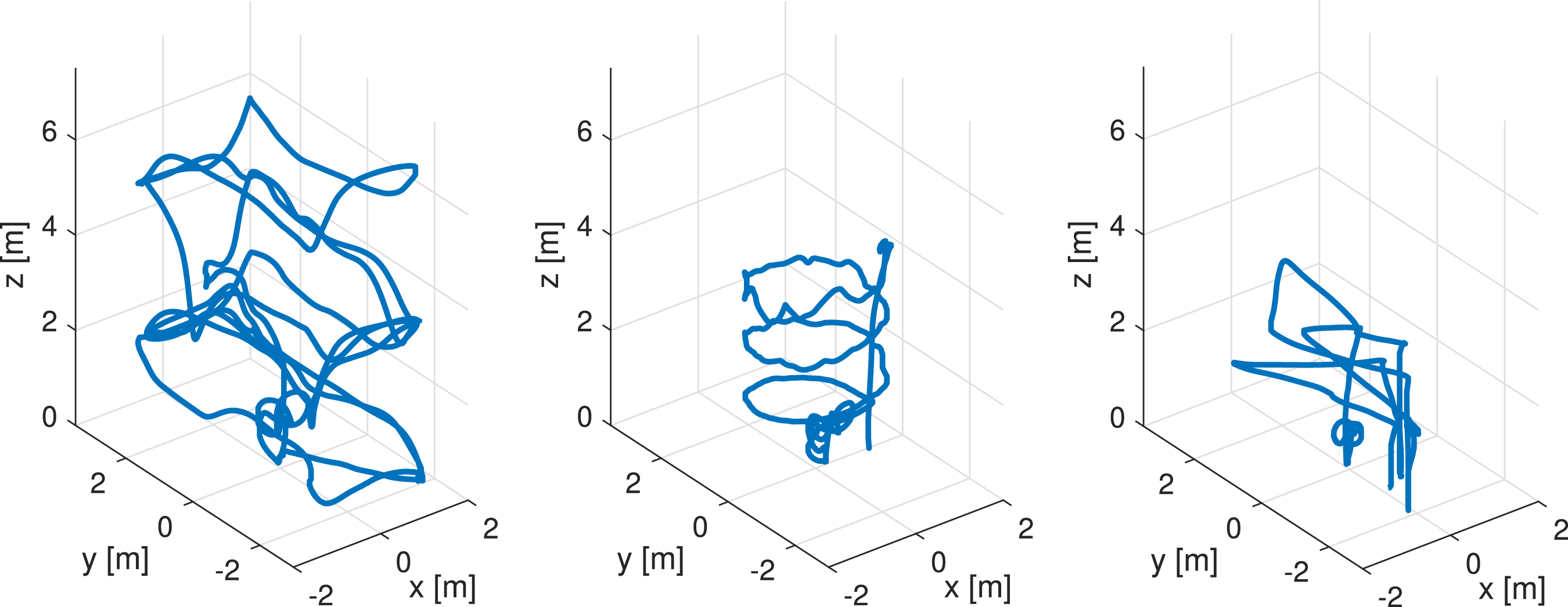Left: Ascending square trajectory, Middle: Upwards spiral, Right: Translations with pick and place elements.

4.1.2. Outdoor to indoor transition

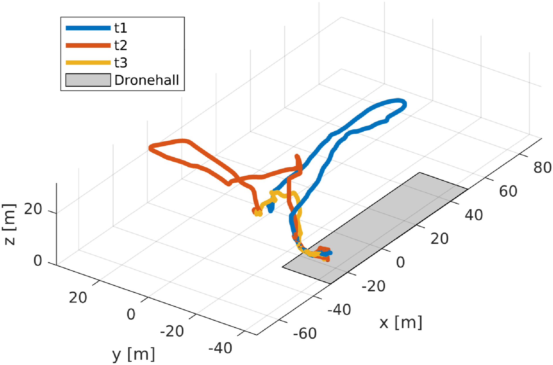
The outdoor to indoor transition experiments are performed in the surrounding outdoor area, and the indoor area of the Dronehall. This location made use of the fiducial marker setup as described in Section 3.2.6. The transition datasets provide a variety of flight patterns. All datasets start at approximately the same location. Figure 17 illustrates individual flight sectors and Figure 18 shows the recorded trajectories and map overlays.

Figure 17.

Location map and flight sectors for the Klagenfurt Dronehall indoor - outdoor transition experiments. Map source: Land Kaernten - KAGIS ⁸

Figure 18.

Trajectory and overlays for the outdoor to indoor transition datasets. The shaded area marks the indoor area.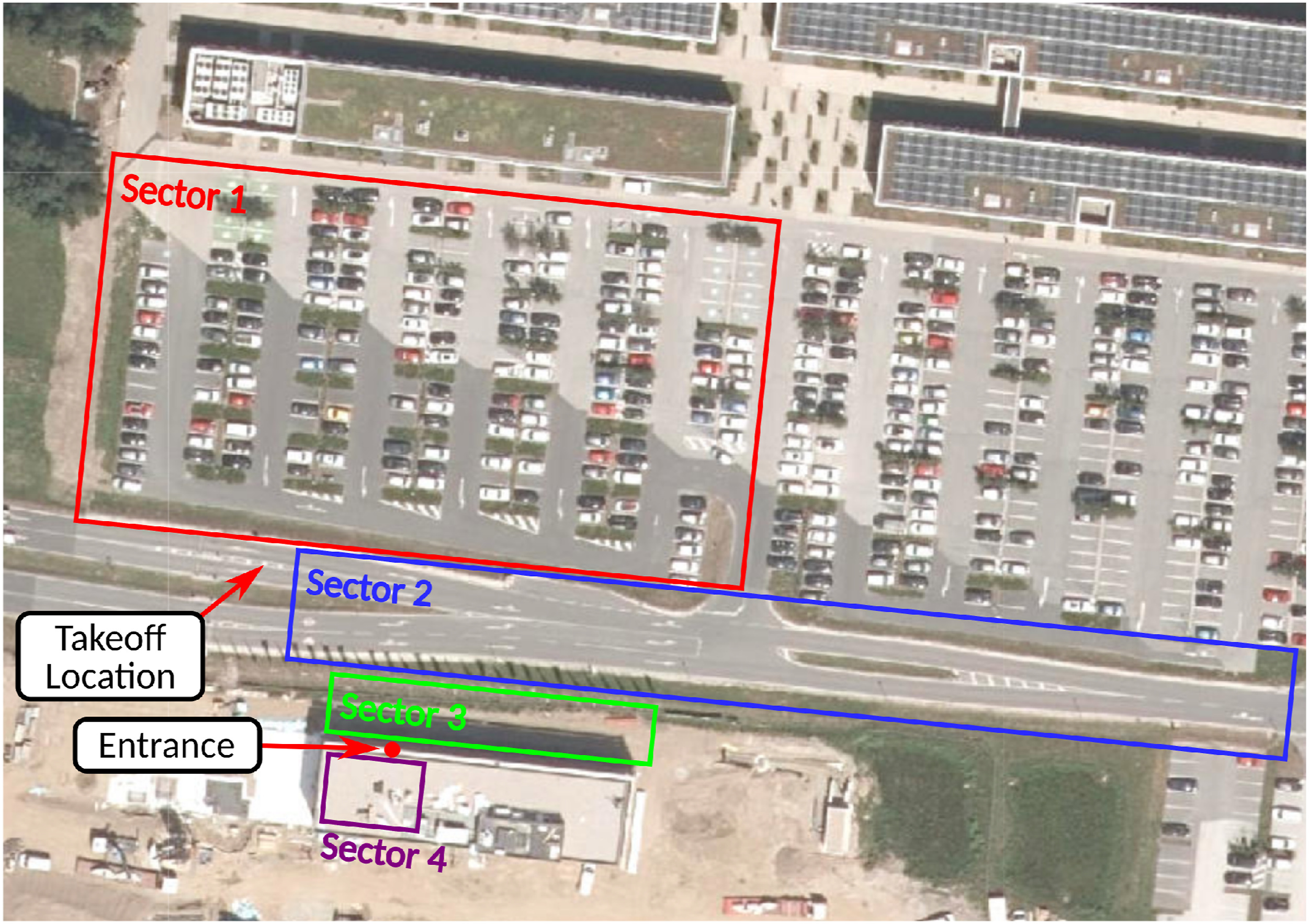

Sectors 1 and 2 are the main outdoor areas of the science park of the university. Sector 3 is the transition area in which the GNSS quality starts to degrade based on the altitude of the vehicle. The lower the position of the vehicle, the higher the GNSS signal occlusion due to the building. Figure 19 further illustrates the GNSS signal degradation as the vehicle moves closer to the building at ground level. Sector 4 represents the indoor location of the Dronehall. The process of gaining and losing the RTK fix of the GNSS modules shows a hysteresis effect. Once the observation of satellites is lost after a longer period, regaining the same accuracy is not instantaneous and requires significant time.

Figure 19.

This map illustrates the RTK GNSS accuracy in close proximity to the Dronehall building. Red dots show the XY position at which the measurements are taken, and the z-axis shows the sample standard deviation of different static measurement sequences with more than 2000 position measurements each. The surface shows the nearest interpolation of the data points, and the blue dot indicates the location of the entrance. This shows that the position accuracy towards the building degrades as expected. It also shows that the accuracy is sufficient between four and eight meters, which is the area where the fiducial markers are placed for ground truth during the transition phase.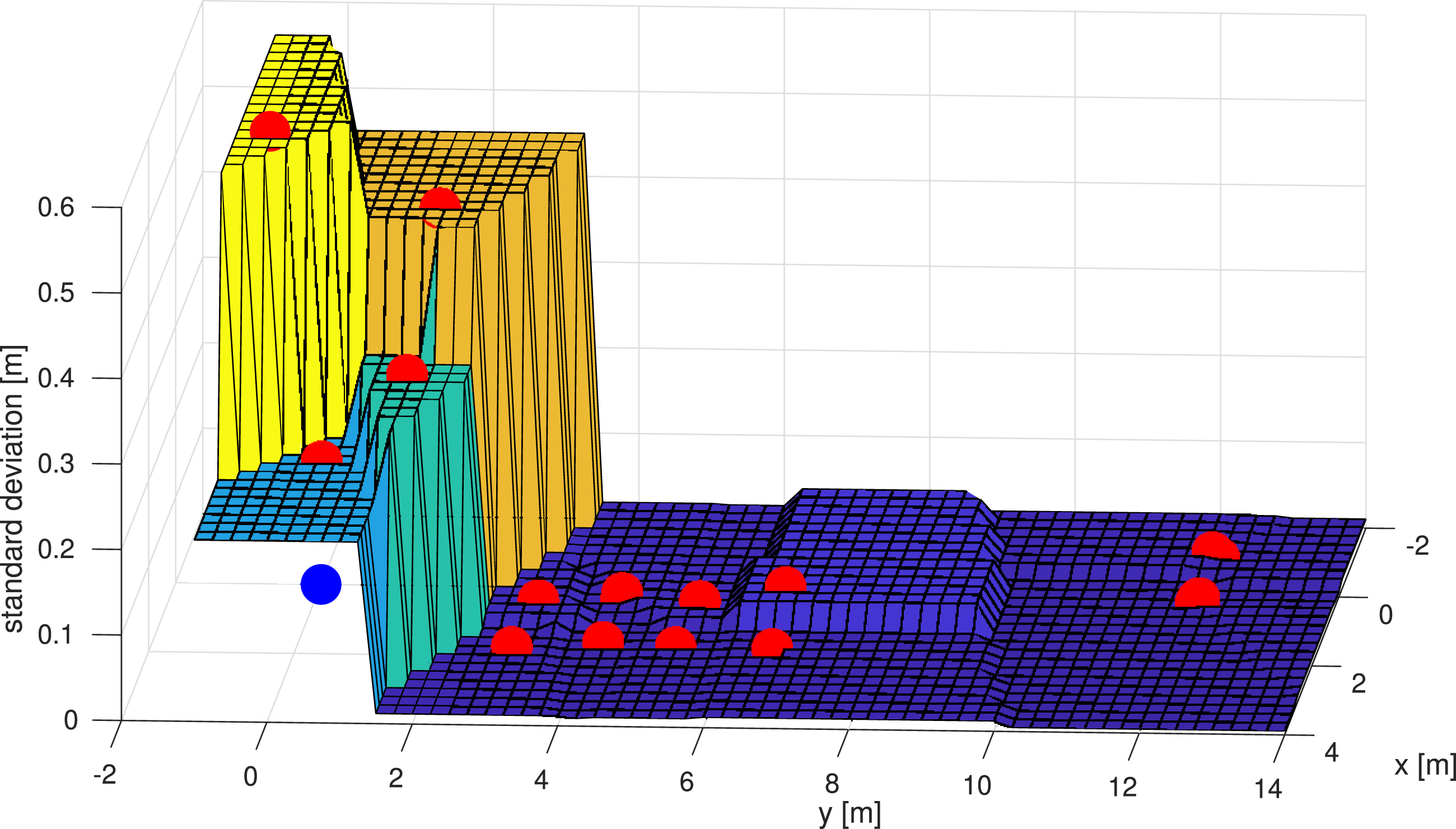

Datasets were recorded throughout the day, which resulted in varying light conditions between recordings. The lighting conditions for the transition datasets are especially challenging. Sectors 1 and 2 provide natural light and possible reflections from the ground varying based on the height and rotation of the vehicle. Sector 3 has shadow casting because of the nearby building, and Sector 4 provides artificial light after transitioning to the indoor location. As described in Section 3.2.3, the exposure time of the navigation camera was fixed and as low as possible to prevent motion blur. The gain was set to “auto” with a reference value that provides the best result for the changing light conditions. The majority of trajectories perform a square over Sectors 1 and 2 before transitioning to the indoor location, starting at a high altitude of 20 m. One dedicated dataset also provides a constant velocity segment along Sector 2, to expose possible unobservability for VIO algorithms. A subsection of datasets also shows lens flare effects for the stereo camera when facing the sun at high altitudes.

Another real-world effect is the change of the magnetic field strength when transitioning from indoor to outdoor due to the influence of the building structure. Figure 20 shows the change of the magnetic field strength during one transition. Such real-world effects are desired and highly relevant for the development of real-world applications. The presented work will enable the development and deployment of robust solutions to work with such effects.

Figure 20.

This graph shows the change of the magnetic field during the transition phase from outdoor to indoor. Such real-world effects can either be treated as outliers or as additional information to adapt to changing magnetic field as described by Brommer et al. (2020).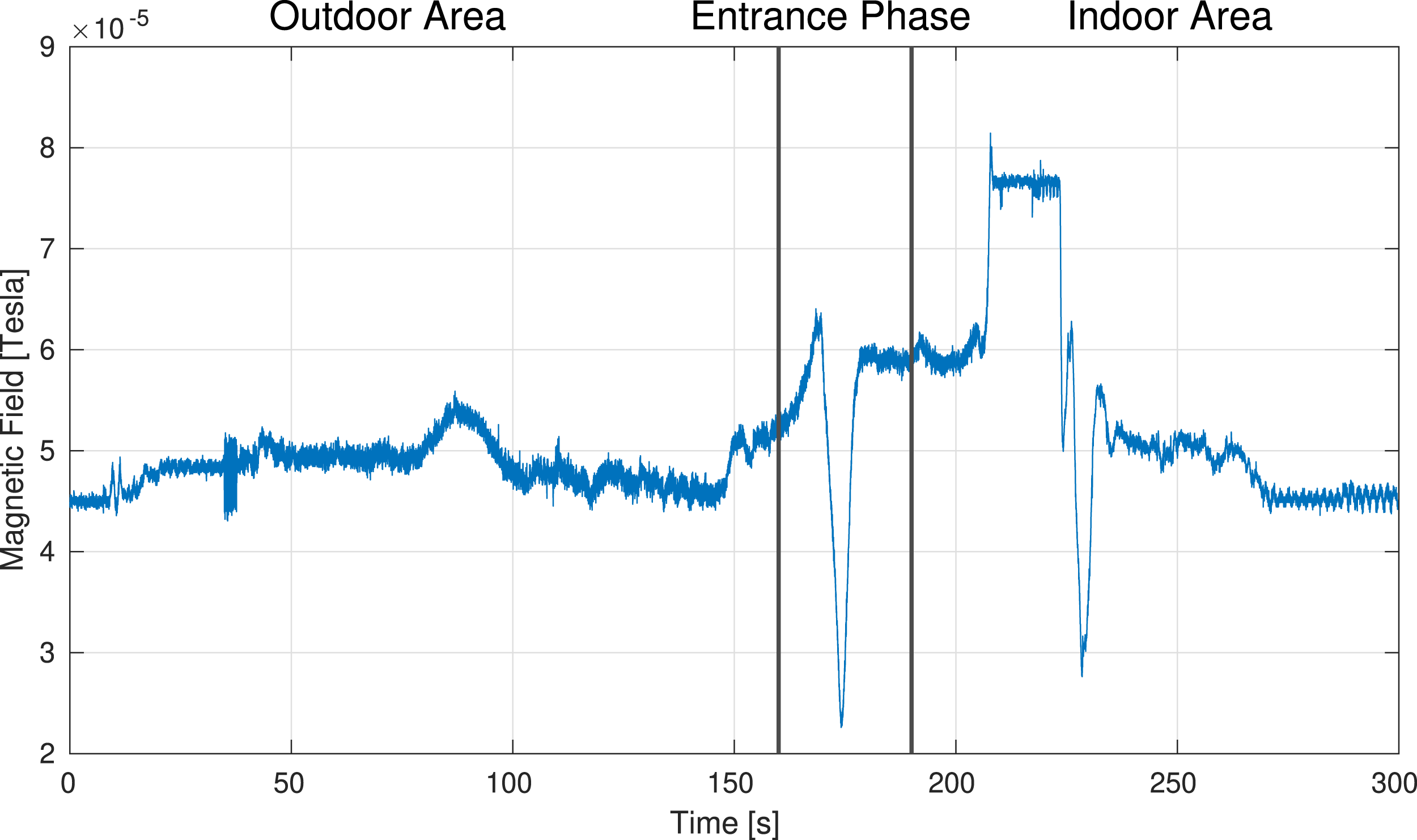

4.2. Model airfield Klagenfurt

The location at the model airfield in Klagenfurt, with the environmental information summarized by Table 3, provides a purely outdoor dataset with partially visible fiducial marker and UWB modules. These data sequences focus on a simplified scenario for visual inertial odometry and UWB triangulation. The environment mainly provides a planar grass field with a partial agricultural area. Similar to the outdoor-indoor transition setup, the three UWB modules are mounted on fiducial marker boards to calculate a global reference. However, instead of using a motion capture system, the GNSS-based ground truth is used to express the location of the board and the UWB module position consecutively.

4.3. Mars analog desert

The desert location at the Ramon crater in Israel was used for the Mars analog simulation AMADEE20 ⁹ and was the experiment area for the Mars analog Helicopter experiments. The experiments were performed in a wider area, but information on a general environmental reference point is shown by Table 4.

While the recorded sequences can be used as a multi-sensor setup without relation to off-world experiments, we want to highlight the specific high-level aspects regarding the Mars analog datasets concerning the environment, the sensor setup, and the design of the experiments. The sensor setup of the vehicle includes an LRF co-mounted with the navigation camera to resemble the specific sensor setup of the Mars-Helicopter Ingenuity.

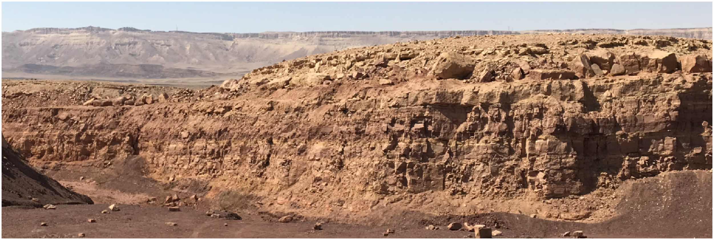
The properties of the environment, such as the terrain topographies, rock distribution, granularity, coloring of the sediment structures, and other environmental parameters, are deemed to be similar to a Mars environment, according to the Austrian Space Forum Grömer (2022). The datasets cover scenarios for different surface properties ranging from flat and sand-only surfaces to flat and stone-paved patches, as illustrated by Figure 21. Special attention was also given to terrain structures with high elevation, such as small canyons, craters, and crater walls (see Figure 22). This environment does not feature external synthetic visual cues or sensors such as UWB modules. The only external component was the RTK GNSS base station.

Figure 21.

Externally recorded images as a reference for terrain structures. The top row shows the topography, and the bottom row shows a close-up of the ground structure. Left: Sand patches and no terrain, Middle: Stone-paved medium terrain, Right: High terrain elevation and sandy ground structure.

Figure 22.

Representative image of a crater wall in the Negev desert. This location, among others was used to record data for a possible crater wall mapping task. The image was taken with an external device.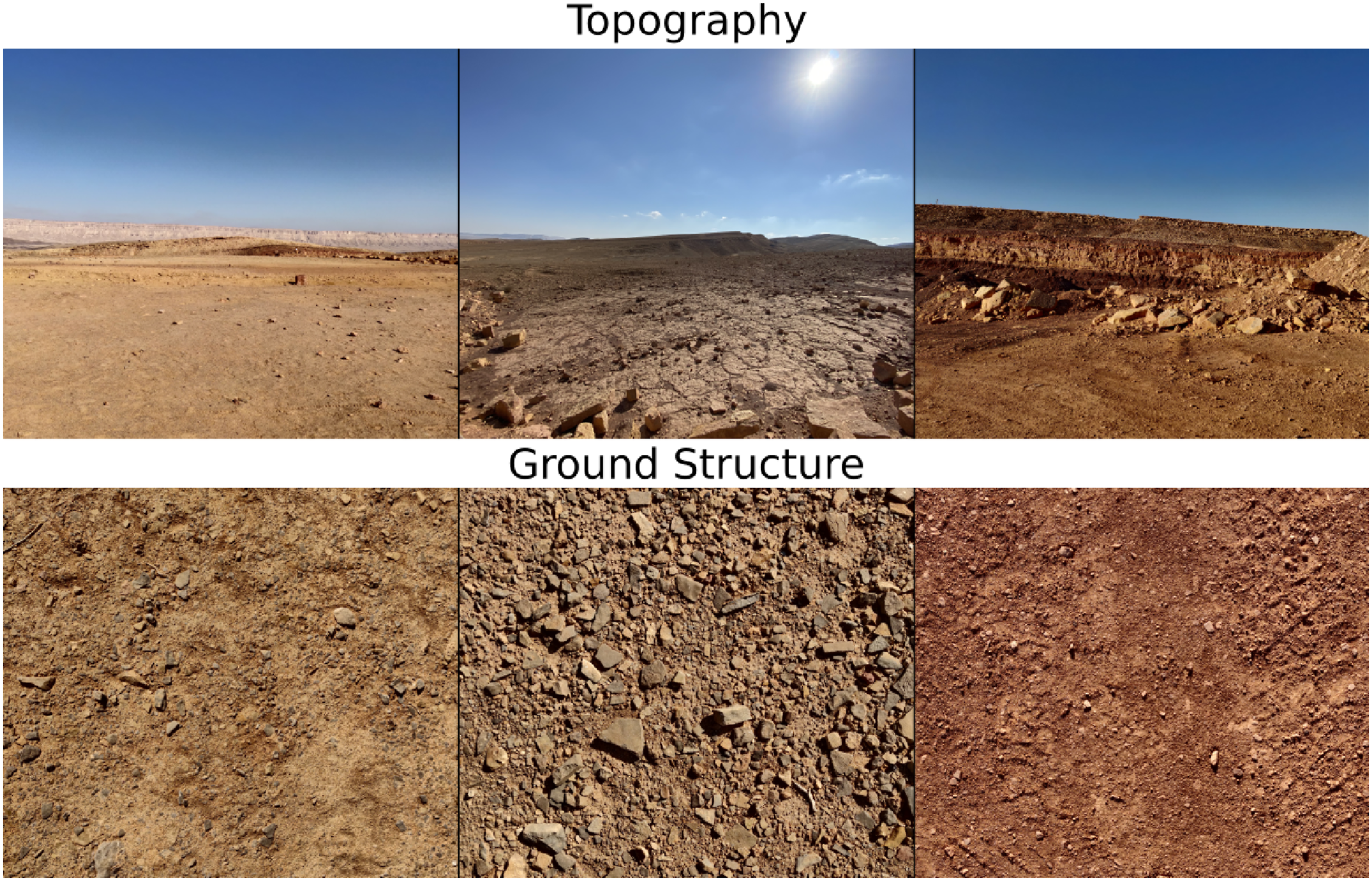

Experiments were designed to cover Mars analog relevant scientific flight tasks and difficulties. Thus, experiments include science close-up flights with transitions from intermediate altitude towards an object such as a rock, a semi-circular scan of the object, and consecutive raises to the initial altitude. Another experiment for the acquisition of scientific data is scans of crater walls. The Mars helicopter is predestined for such tasks because rovers were not able to record imagery of sediment layers at close proximity and high elevation. Thus, datasets 9, 13, and 14 provide longer horizontal traverses along crater walls with the 3D camera facing the wall. Both experiment types can be used for mapping and 3D reconstruction. In addition to the camera-based information, we also performed experiments that pose challenges because of the flight patterns and the environment. These experiments include higher speed traverse at high altitude, constant velocity segments to challenge observability aspects of localization algorithms, and crater wall fly-overs for abrupt and relative elevation changes.

Figure 23 shows the majority of flight patterns performed in the Ramon Crater. The flights were performed in three distinct zones. Zone one is the location of the habitat and had semi-structured ground and terrain with the exception of a crater wall, which was used for trajectories with high relative altitude changes and vertical movement along the crater wall for possible mapping and 3D reconstruction. Zone two has terrain with step elevation changes in the form of a canyon. This zone was used for lateral crater wall recordings and long distances with higher altitude flights. The ground structure in zone three was a planar ground with low texture and was used for low-altitude science close-ups and multiple lateral traverse flights.

Figure 23.

Trajectory and map overlays for the Mars analog datasets. Zone 1 shows the habitat in a small valley where a part of the cliff mapping data was recorded. Zone 2 shows a steep and lengthy canyon in which cliff mapping data and data with high elevation changes were acquired. Zone 3 was a planar-only region that was also used for the science close-up maneuvers. - Map ⓒ OpenStreetMap contributors.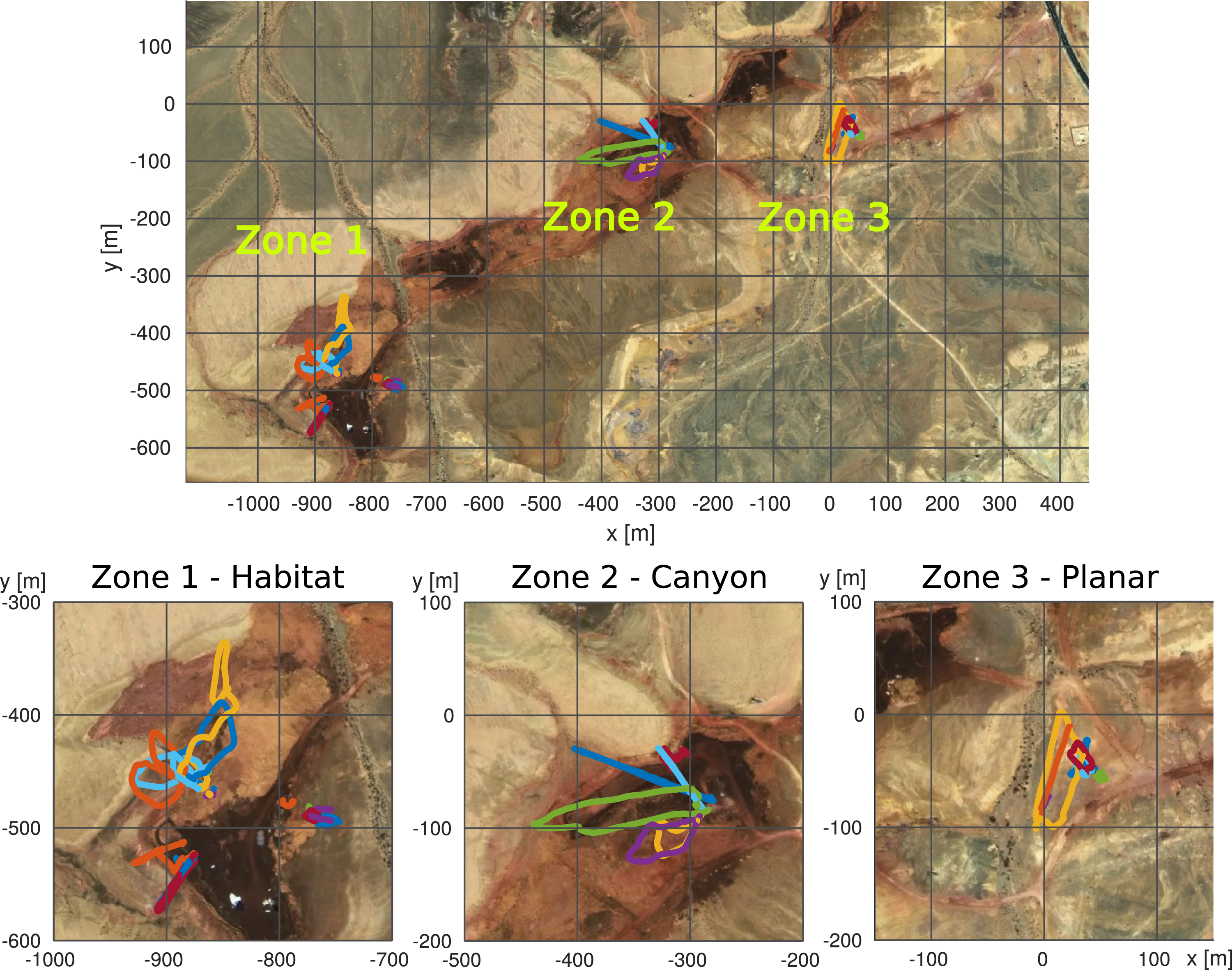

4.4. Datasets

This section describes the patterns and scenarios which were performed for each location. In general, the majority of datasets have an initialization phase. This initialization phase consists of a smooth impulse in the direction of the IMU’s z-axis and consecutive smooth excitations in 6 DoF. This can be used for VIO algorithms requiring initial IMU excitement and for initial convergence. However, since this feature is not desired in all cases, the copter is placed down to the ground after initialization, followed by a short steady pause before the actual flight maneuver. Thus, the initial phase can be cropped. A list of the majority of recorded flights is shown in Table 5.

Table 5.

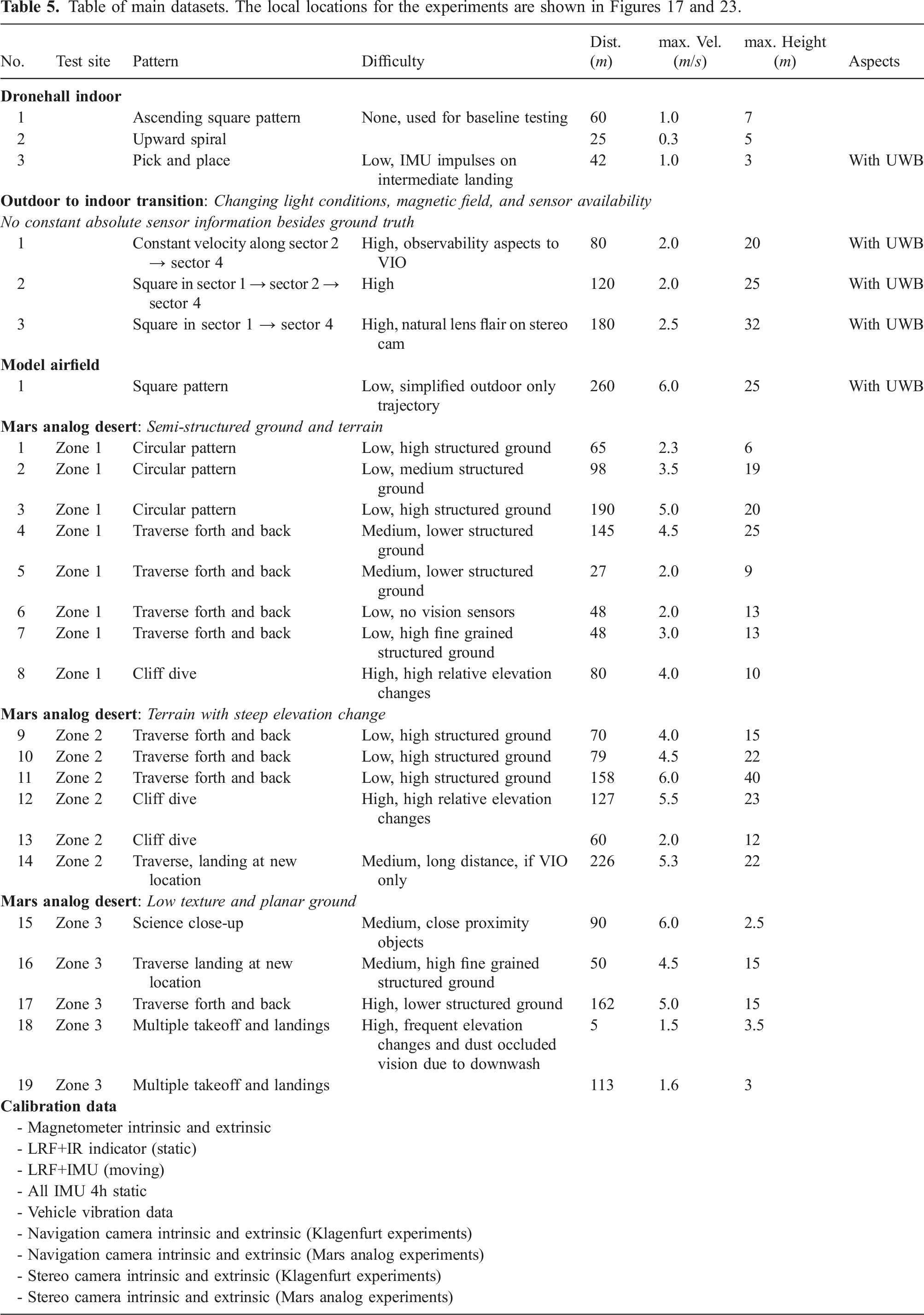
Table of main datasets. The local locations for the experiments are shown in Figures 17 and 23.

No.	Test site	Pattern	Difficulty	Dist. (m)	max. Vel. (m/s)	max. Height (m)	Aspects
Dronehall indoor
1		Ascending square pattern	None, used for baseline testing	60	1.0	7
2		Upward spiral		25	0.3	5
3		Pick and place	Low, IMU impulses on intermediate landing	42	1.0	3	With UWB
Outdoor to indoor transition: Changing light conditions, magnetic field, and sensor availability
No constant absolute sensor information besides ground truth
1		Constant velocity along sector 2 → sector 4	High, observability aspects to VIO	80	2.0	20	With UWB
2		Square in sector 1 → sector 2 → sector 4	High	120	2.0	25	With UWB
3		Square in sector 1 → sector 4	High, natural lens flair on stereo cam	180	2.5	32	With UWB
Model airfield
1		Square pattern	Low, simplified outdoor only trajectory	260	6.0	25	With UWB
Mars analog desert: Semi-structured ground and terrain
1	Zone 1	Circular pattern	Low, high structured ground	65	2.3	6
2	Zone 1	Circular pattern	Low, medium structured ground	98	3.5	19
3	Zone 1	Circular pattern	Low, high structured ground	190	5.0	20
4	Zone 1	Traverse forth and back	Medium, lower structured ground	145	4.5	25
5	Zone 1	Traverse forth and back	Medium, lower structured ground	27	2.0	9
6	Zone 1	Traverse forth and back	Low, no vision sensors	48	2.0	13
7	Zone 1	Traverse forth and back	Low, high fine grained structured ground	48	3.0	13
8	Zone 1	Cliff dive	High, high relative elevation changes	80	4.0	10
Mars analog desert: Terrain with steep elevation change
9	Zone 2	Traverse forth and back	Low, high structured ground	70	4.0	15
10	Zone 2	Traverse forth and back	Low, high structured ground	79	4.5	22
11	Zone 2	Traverse forth and back	Low, high structured ground	158	6.0	40
12	Zone 2	Cliff dive	High, high relative elevation changes	127	5.5	23
13	Zone 2	Cliff dive		60	2.0	12
14	Zone 2	Traverse, landing at new location	Medium, long distance, if VIO only	226	5.3	22
Mars analog desert: Low texture and planar ground
15	Zone 3	Science close-up	Medium, close proximity objects	90	6.0	2.5
16	Zone 3	Traverse landing at new location	Medium, high fine grained structured ground	50	4.5	15
17	Zone 3	Traverse forth and back	High, lower structured ground	162	5.0	15
18	Zone 3	Multiple takeoff and landings	High, frequent elevation changes and dust occluded vision due to downwash	5	1.5	3.5
19	Zone 3	Multiple takeoff and landings		113	1.6	3
Calibration data
- Magnetometer intrinsic and extrinsic
- LRF+IR indicator (static)
- LRF+IMU (moving)
- All IMU 4h static
- Vehicle vibration data
- Navigation camera intrinsic and extrinsic (Klagenfurt experiments)
- Navigation camera intrinsic and extrinsic (Mars analog experiments)
- Stereo camera intrinsic and extrinsic (Klagenfurt experiments)
- Stereo camera intrinsic and extrinsic (Mars analog experiments)

4.5. Vehicle vibration analysis

It is well known that parasitic effects in measured inertial data can lead to drastic decreases in performance of classical state estimation methods if not accounted for. Apart from noise and biases of the inertial sensor itself, these also include vibrations of the vehicle that couple into the IMU at various frequencies. One major source of vibrations on UAVs are the motors. While it may be difficult to completely account for vibrations in classical state estimation approaches, it has been hypothesized that latent features in IMU data such as RPM or velocity dependent vibrations are beneficial for learning-based methods Chen et al. (2018); Steinbrener et al. (2022). In this section, we show that the motors introduce a resonant frequency in the IMU spectrum that is characteristic of their speed. This resonance is particularly pronounced in the inertial data obtained from the high-rate IMU.

During flight, the PX4 provides the rate values for each of the four motors at 100 Hz. The PX4 rate values range from 0 to 2000 on a scale with arbitrary units. To calibrate these rate values to actual RPM values, the data obtained with the vibration measurement setup described in Section 3.3 for seven different motor speeds is used to derive an analytic relationship between PX4 rate values and measured RPM. The corresponding data is shown in Table 6, and plotted on the left hand size of Figure 24 together with a quadratic polynomial with coefficients a₀ = 168.5541, a₁ = 12.1870, and a₂ = −0.0023.

Table 6.

RPM calibration.

Relative RPM	PX4 rate values	Measured RPM
10%	297	3560
20%	486	5605
40%	864	9000
60%	1242	11800
80%	1620	14000
100%	1999	15500

Figure 24.

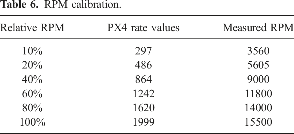
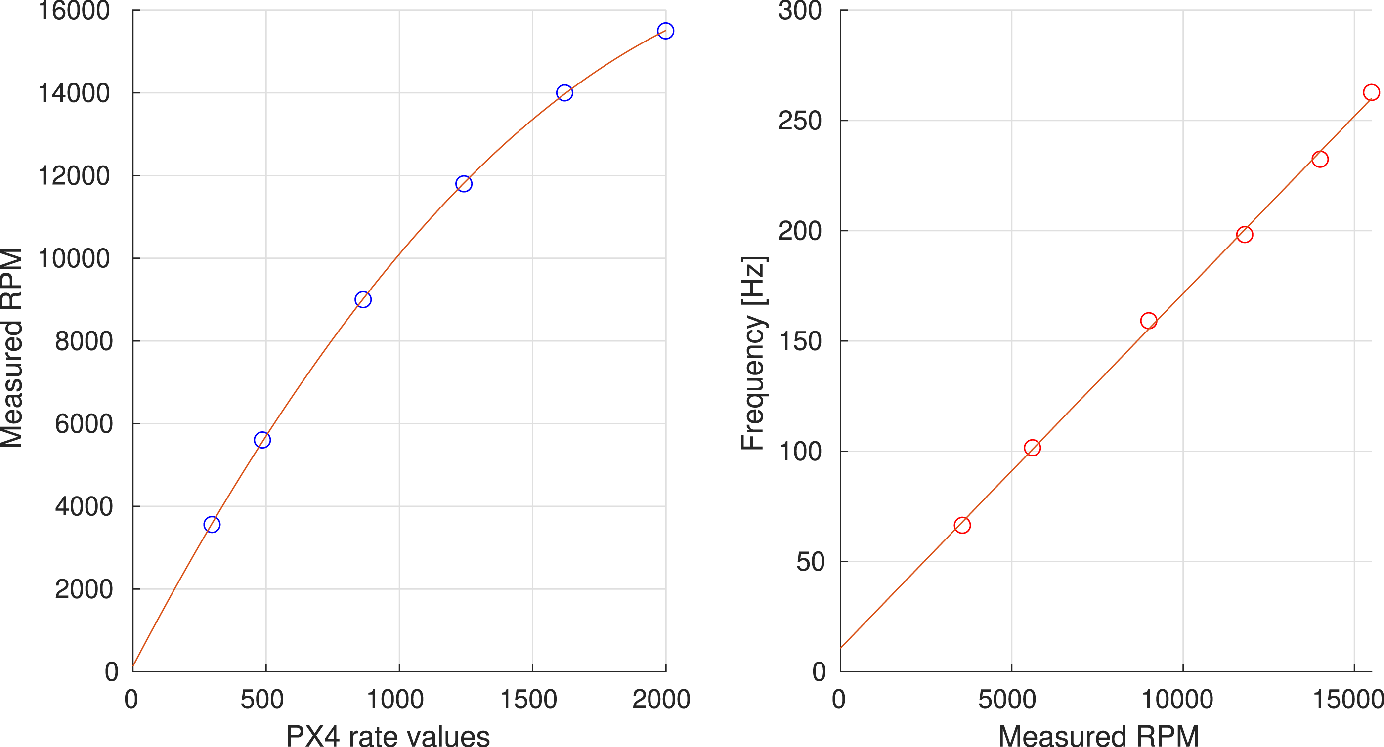
Calibration of PX4 rate values (left), and resonant frequencies as a function of motor RPM (right).

To analyze the frequencies of the resonances for the different motor speeds, we computed the averaged power spectral densities of the high-rate inertial data for each vibration test run using Matlab’s spectrogram method, and extracted the frequency of the main peak using Matlab’s findpeaks method. Plotting the true motor RPMs against the peak frequencies shows a linear relationship. The corresponding line fit with coefficients a₀ = 10.6666 and a₁ = 0.0161 is shown on the right side of Figure 24 along with the data. Although this data was recorded in a very controlled experimental setup, a clear relationship between the resonance in the spectrogram and the PX4 motor rate values exists also for real-flight data. Figure 25 shows the spectrogram of the high-rate IMU for one of the flights in gray. Overlaid in color are the expected resonances computed from the reported PX4 rate values for each motor using the same linear fit parameters. The inset shows a magnified portion of the whole spectrogram. As can be seen, the expected resonant frequencies correlate very well with the observed resonances. We attribute the remaining differences to experimental effects in the real-flight scenario. In particular, the actual RPMs may differ from the PX4 rate values. Nonetheless, these results indicate the presence of motor speed dependent resonances in the recorded inertial data that can be of interest in particular to the learning community.

Figure 25.

Prediction of spectral resonances based on PX4 rate values (color) and measured resonances (gray) for real-flight data.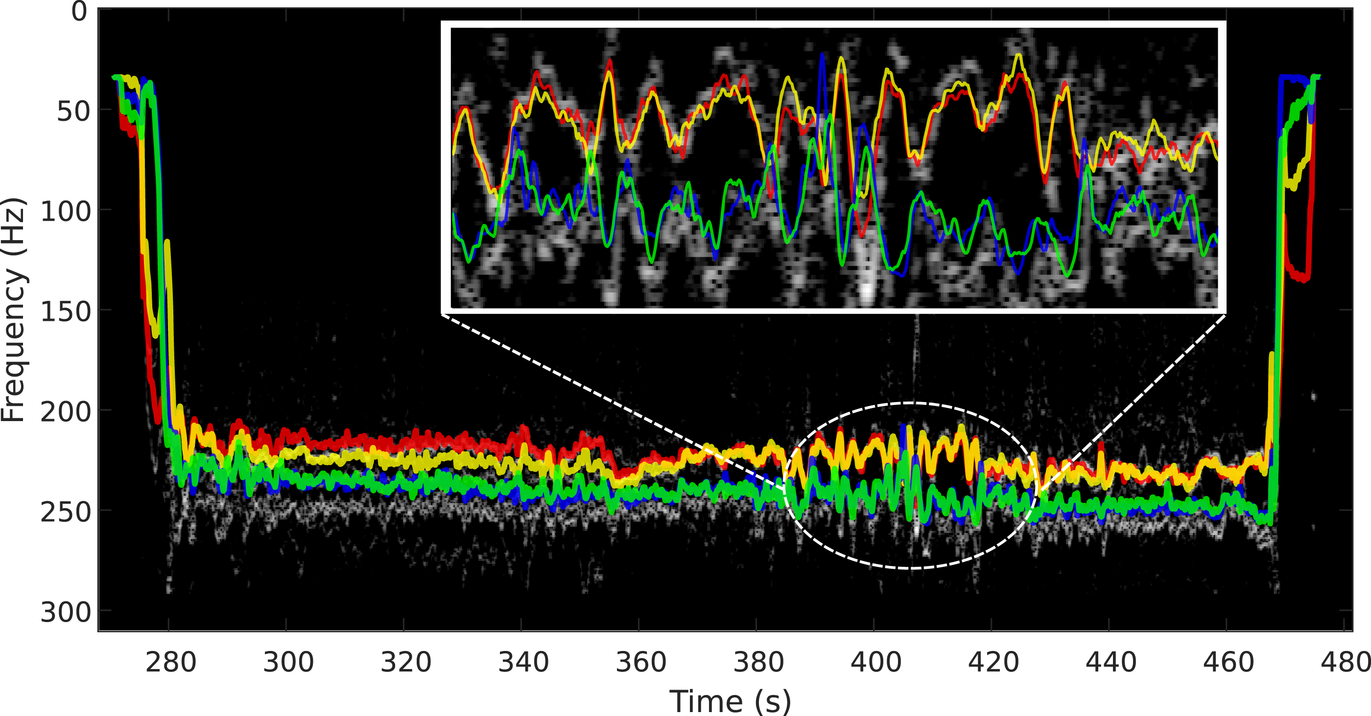

5. Ground truth

This section describes the generation of 6 DoF ground truth data for the outdoor datasets, sensor time calibration, as well as the alignment of the pose information for the outdoor to indoor transition datasets. The tools which were used to generate the ground truth will be open-sourced together with this dataset.

5.1. Notation

The notation of transformations used by this work is as follows. ${\mathbf{R}}_{\mathrm{A} \mathrm{B}}$ is the rotation of frame B expressed in frame A. ${}_{\mathrm{A}}{\mathbf{p}}_{\mathrm{A} \mathrm{B}}\equiv {\mathbf{p}}_{\mathrm{A} \mathrm{B}}$ is the translation from frame A to B expressed in frame A. As an example ${}_{\mathrm{C}}{\mathbf{p}}_{\mathrm{A} \mathrm{B}}={\mathbf{R}}_{\mathrm{C} \mathrm{A}}{}_{\mathrm{A}}{\mathbf{p}}_{\mathrm{A} \mathrm{B}}$ .

Respective homogeneous transformations are defined by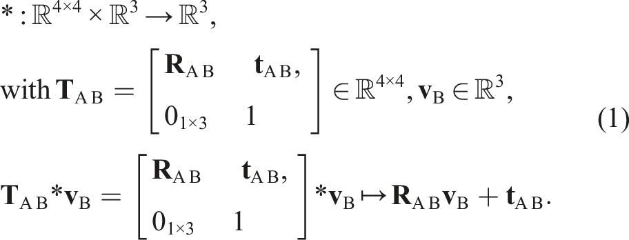

$\begin{array}{l}*:{\mathbb{R}}^{4\times 4}\times {\mathbb{R}}^3\to {\mathbb{R}}^3,\\ \text{with}\hspace{0.17em}{\mathbf{T}}_{\mathrm{A} \mathrm{B}}=\left[\begin{array}{ll}{\mathbf{R}}_{\mathrm{A} \mathrm{B}}& {\mathbf{t}}_{\mathrm{A} \mathrm{B}},\\ 0_{1\times 3}& 1\end{array}\right]\in {\mathbb{R}}^{4\times 4},{\mathbf{v}}_{\mathrm{B}}\in {\mathbb{R}}^3,\\ {\mathbf{T}}_{\mathrm{A} \mathrm{B}}*{\mathbf{v}}_{\mathrm{B}}=\left[\begin{array}{ll}{\mathbf{R}}_{\mathrm{A} \mathrm{B}}& {\mathbf{t}}_{\mathrm{A} \mathrm{B}},\\ 0_{1\times 3}& 1\end{array}\right]*{\mathbf{v}}_{\mathrm{B}}\mapsto {\mathbf{R}}_{\mathrm{A} \mathrm{B}}{\mathbf{v}}_{\mathrm{B}}+{\mathbf{t}}_{\mathrm{A} \mathrm{B}}.\end{array}$

(1)

5.2. Vehicle 6 DoF pose

As mentioned before, we chose to use individual raw measurements for the generation of the ground truth data because of the high measurement accuracy. Using a recursive algorithm or a graph-based optimization for ground truth data generation can cause biased results for comparisons against this ground truth data. Original raw sensor data is provided to allow the use of different methods for the generation of ground truth.

We aim to generate 6 DoF ground truth information of an IMU frame with respect to the GNSS world-frame (ENU). The provided ground truth for the vehicle is referenced to the PX4 IMU. This is done based on two GNSS position measurements and a known calibration of the GNSS antenna positions with respect to the IMU-frame. The method relies on the generation of a virtual GNSS sensor frame, which provides 6 DoF. The calculation of the pose for the IMU frame is then achieved by applying transformations of known calibration transformations. Using the two position measurements and generating a virtual directional vector, this setup only provides rotational information in 2 DoF. Thus, we are using the measurements of the directional magnetic vector as support and to fix the ground truth frame for a 3 DoF rotation. As a result, this method will lead to a full-frame definition in 3D with 3 DoF orientation and 3 DoF position. The reference frames and sensor information for the ground truth method are shown in Figure 26. For the remainder of this document, the world-frame {W} is equal to the GNSS world-frame, following the East-North-Up (ENU) convention ENU → XYZ. The virtual GNSS frame {VG}, IMU/Body frame {I}, and the frame of the magnetic-sensor {M} are placed on a rigid body. The GNSS position measurements ${\mathbf{p}}_{\mathrm{W} \mathrm{G}1}$ and ${\mathbf{p}}_{\mathrm{W} \mathrm{G}2}$ are expressed with respect to the world-frame.

Figure 26.

Ground truth sensor frame setup. RTK GNSS and Magnetometer sensor-frames with respective transformations for the described 6 DoF ground truth calculation.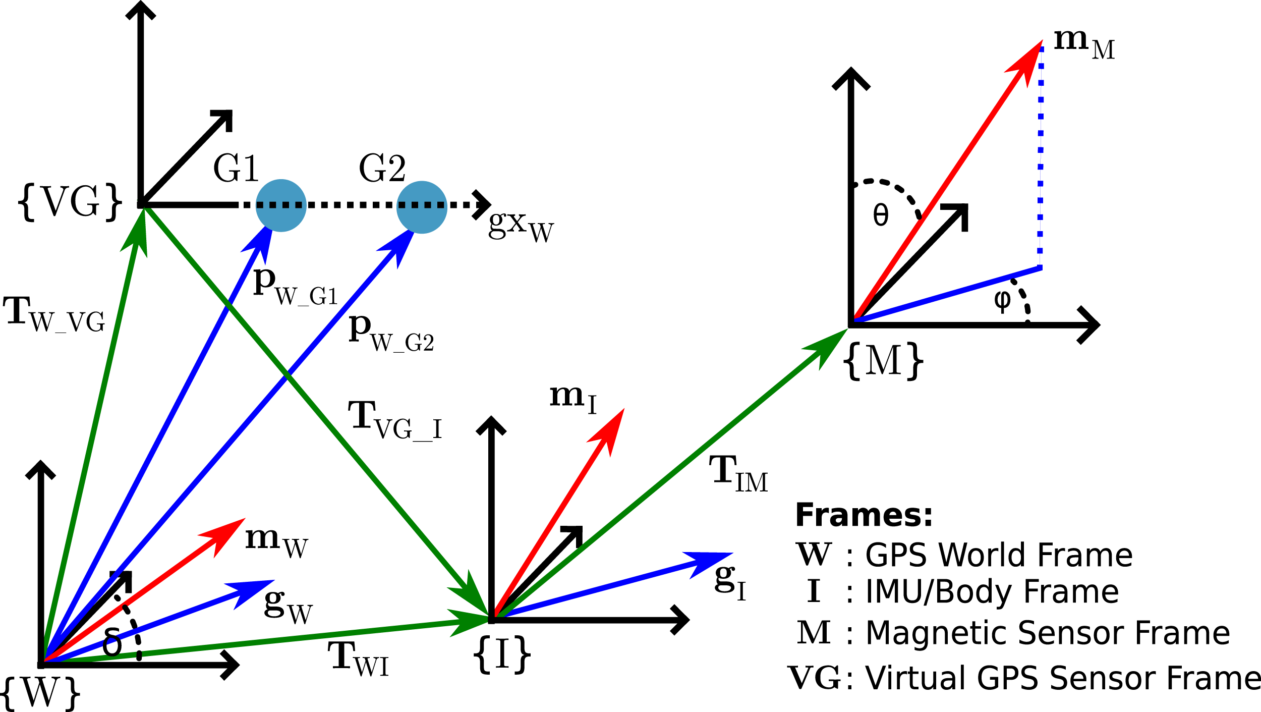

The magnetic field ${\mathbf{m}}_{\mathrm{w}}$ is assumed to be locally static with respect to the world-frame and the local magnetic variation, that is, the inclination and declination, is known. In the IMU frame, the magnetic variation depends on the rotation of the vehicle. This effect needs to be taken into account. Thus, a system that describes the rotation of the vehicle needs to use the following set of information: The magnetic vector expressed in the IMU and the world-frame ${\mathbf{m}}_{\mathrm{w}}$ and ${\mathbf{m}}_{\mathrm{i}}$ , respectively, as well as the virtual GNSS vectors in world and IMU frame ${\mathbf{g}}_{\mathrm{w}}$ and ${\mathbf{g}}_{\mathrm{i}}$ , respectively. Since only direction is relevant, all vectors are normalized for this analysis. In addition, we can make use of the orthogonal vectors ${\mathbf{c}}_{\mathrm{w}}={\mathbf{g}}_{\mathrm{w}}\times {\mathbf{m}}_{\mathrm{w}}$ and ${\mathbf{c}}_{\mathrm{i}}={\mathbf{g}}_{\mathrm{i}}\times {\mathbf{m}}_{\mathrm{i}}$ which renders a possible linear least squares problem full-rank. We present three different methods to analyze the resulting data. The naive approach is to solve the resulting linear least squares problem directly:

$\begin{array}{ll}\mathbf{y}& =\mathbf{A}\hspace{0.17em}\mathbf{x}\end{array}$

(2)

$\left[{\mathbf{g}}_{\mathrm{w}};\hspace{0.17em}{\mathbf{m}}_{\mathrm{w}};\hspace{0.17em}{\mathbf{c}}_{\mathrm{w}}\right]={\mathbf{R}}_{\mathrm{w} \mathrm{i}}\left[{\mathbf{g}}_{\mathrm{i}};\hspace{0.17em}{\mathbf{m}}_{\mathrm{i}};\hspace{0.17em}{\mathbf{c}}_{\mathrm{i}}\right]$

(3)

However, an additional adaptation is needed because the result is not guaranteed to be a rotation matrix. Another approach is given by the following system, which allows a non-linear optimization on the tangent space and ensures that the result is a rotation matrix:

$\left[\begin{array}{l}{\mathbf{g}}_{\mathrm{w}}\\ {\mathbf{m}}_{\mathrm{w}}\\ {\mathbf{c}}_{\mathrm{w}}\end{array}\right]=\left[\begin{array}{lll}{e}^{\lfloor \mathit{\omega }\rfloor }& 0& 0\\ 0& e^{\lfloor \mathit{\omega }\rfloor }& 0\\ 0& 0& e^{\lfloor \mathit{\omega }\rfloor }\end{array}\right]\left[\begin{array}{l}{\mathbf{g}}_{\mathrm{i}}\\ {\mathbf{m}}_{\mathrm{i}}\\ {\mathbf{c}}_{\mathrm{i}}\end{array}\right]$

(4)

With Jacobian:

$\frac{\partial }{\partial \mathit{\omega }}h\left(\mathit{\omega }\right)=\left[\begin{array}{lll}-e^{\lfloor \mathit{\omega }\rfloor } \lfloor {\mathbf{g}}_{\mathrm{i}}\rfloor ;& -e^{\lfloor \mathit{\omega }\rfloor }\lfloor {\mathbf{m}}_{\mathrm{i}}\rfloor ;& -e^{\lfloor \mathit{\omega }\rfloor } \lfloor {\mathbf{c}}_{\mathrm{i}}\rfloor \end{array}\right]$

(5)

Finally, our preferred method because of its simplicity forms a least squares problem according to Wahba’s problem Wahba (1965). This approach ensures a rotation matrix and allows to introduce weights for individual inputs. For the present application, it is of interest to associate a higher weight to the GNSS-based information because it is less likely to be disturbed by the environment in contrast to the magnetometer. The magnetometer measurements only serve the purpose of supporting the third degree of freedom for the orientation information. The weight α for the GNSS vector is chosen heuristically and is set to 50:1.

$\begin{array}{ll}\mathbf{A}& =\alpha \hspace{0.17em}{\mathbf{g}}_{\mathrm{w}}\hspace{0.17em}{\mathbf{g}}_{\mathrm{i}}^{ \mathrm{T}}+{\mathbf{m}}_{\mathrm{w}}\hspace{0.17em}{\mathbf{m}}_{\mathrm{i}}^{ \mathrm{T}}+{\mathbf{c}}_{\mathrm{w}}\hspace{0.17em}{\mathbf{c}}_{\mathrm{i}}^{ \mathrm{T}}\end{array}$

(6)

$\begin{array}{ll}\mathbf{A}& =\mathbf{US}{\mathbf{V}}^{\mathrm{T}}\end{array}$

(7)

$\begin{array}{ll}\mathbf{R}& =\mathbf{UM}{\mathbf{V}}^{\mathrm{T}}\end{array}$

(8)

$\begin{array}{ll}\text{with}\hspace{0.17em}\mathbf{M}& =\text{diag}\left(\left[\begin{array}{lll}1;& 1;& \det \left(\mathbf{U}\right)\det \left(\mathbf{V}\right)\end{array}\right]\right)\end{array}$

(9)

The position of the IMU expressed in the world-frame, given that GNSS point measurement G2 is the origin of the virtual GNSS frame, is then calculated based on

$\begin{array}{ll}{\mathbf{p}}_{\mathrm{W} \mathrm{G}2}& ={\mathbf{T}}_{\mathrm{W} \mathrm{I}}*{\mathbf{p}}_{\mathrm{I} \mathrm{G}2}\end{array}$

(10)

$={\mathbf{T}}_{\mathrm{W} \text{VG}} {\mathbf{T}}_{\text{VG} \mathrm{I}}*{\mathbf{p}}_{\mathrm{I} \mathrm{G}2}$

(11)

$\begin{array}{ll}\Rightarrow {\mathbf{p}}_{\mathrm{W} \mathrm{I}}& ={\mathbf{p}}_{\mathrm{W} \mathrm{G}2}+{\mathbf{R}}_{\mathrm{W} \text{VG}}\hspace{0.17em}{\mathbf{R}}_{\text{VG} \mathrm{I}}\hspace{0.17em}\left(-{\mathbf{p}}_{\mathrm{I} \mathrm{G}2}\right)\end{array}.$

(12)

The three methods for rotation estimation described above are provided with the dataset tools and can be chosen accordingly.

In this context, it is also important to note that the rotation can be incorrect if the magnetometer provides incorrect information. This can be the case where the vehicle is picked up at the beginning of an experiment and the magnetic field is disturbed by the person of the field crew. The increased weight on the GNSS vector when calculating the 3 DoF rotation reduces this effect during this time, and such disturbance does not occur during the main phase of an experiment.

5.3. Sensor time calibration

The synchronization for the computation platforms of the vehicle are described in Section 3.2.8; however, internal system delays can still lead to minor time shifts of the sensor data. Thus, all sensors that are required for the generation of ground truth data are additionally time-synchronized in post-processing. This includes the two RTK GNSS signals, the PX4 IMU and magnetometer, as well as the motion capture system.

To synchronize the two GNSS signals, we first calculate their velocity and use their convolution to find the time offset which provides the highest overlap of the two signals ${\dot{\mathbf{p}}}_{\mathrm{g}1}$ and ${\dot{\mathbf{p}}}_{\mathrm{g}2}$ . Using the synchronized GNSS information, the virtual orientation vector for the two GNSS measurements expressed in the world-frame is built (see the calculation of VG in Section 5.2). In order to synchronize the magnetometer data to the virtual GNSS vector, the time derivative of the horizontal projection for VG and the yaw rotation component measured by the magnetometer are used.

After this step, the time derivative of the rotational ground truth for the outdoor pose information and the motion capture pose is used for the synchronization towards the angular velocity of the PX4 IMU. This provides all sensor time-offsets to generate accurate ground truth information for the vehicle.

5.4. Transition segment alignment

\As described in the previous sections, the indoor ground truth based on motion capture data and the fiducial marker-based position of the vehicle are expressed in the reference frame of the motion capture system because the main marker board is a known motion capture object. Thus, in order to gain continuous ground truth for the transition datasets, only the outdoor pose information based on the RTK GNSS and magnetometer solution and the fiducial marker-based vehicle pose need to be aligned. Since accurate RTK GNSS solutions become sparse towards the entrance of the building, GNSS data from multiple entry approaches are used to increase the accuracy of the alignment. The final alignment between the outdoor GNSS information and the fiducial marker-based trajectory is done by using a least squares solution to Wahba’s problem, shown by, for example, Sorkine and Rabinovich (2017). The resulting ground truth after the alignment is shown by Figure 27. Should this solution be too inaccurate for a specific purpose, the local ground truth for each segment can be used.

Figure 27.

Alignment of the ground truth segments for the outdoor area, the marker-based transition section, and the indoor motion capture pose. The shown trajectory builds the continuous ground truth for the outdoor-indoor datasets.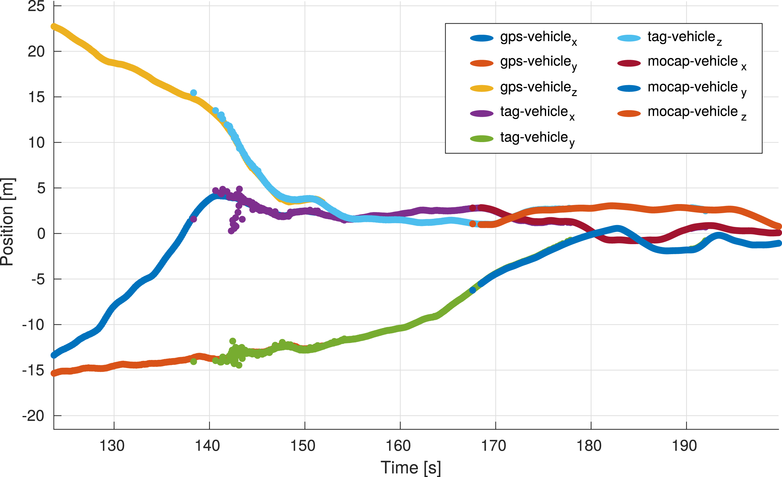

6. Providing the data

The data is provided in human-readable plain text format as dedicated CSV files with headers and uncompressed PNG images with attached timestamps in a CSV file. Individual sensor calibration files are provided in YAML format. The structure of the files is outlined in Figures 30 and 31. A script for the conversion of this data into ROS bagfiles is provided with the toolbox. The generation of other data formats is possible by using the provided script as a template. The calibration of all sensors is provided with respect to the PX4 IMU and allows to construct any relative calibration that might be necessary.

Each outdoor dataset provides two ground truth files. This ground truth is calculated using the RTK GNSS (8 Hz) and the Magnetometer data (80 Hz). Thus, two files are provided, ground_truth_8hz.csv provides data calculated based on RAW GNSS measurements and time-matched magnetometer measurements, while ground_truth_80hz.csv provides data based on interpolated RTK GNSS measurements and the raw magnetometer data. The usage may depend on the scenario and the choice is left to the user. Because the ground truth for the indoor datasets is generated using the motion capture system, ground_truth.csv provides this data for clear association.

The ground truth data for the transition dataset contains the segments for outdoor, transition, and indoor poses. The ground_truth.csv file for these scenarios contains the aligned pose information. Since data from multiple sources with multiple rates are used, the ground truth file also has segments with different frame rates.

Further, all data for individual sensor calibration is provided. This includes static IMU data for the generation of the Allan variance, magnetometer intrinsic calibration data, and camera to IMU calibration sequences.

Measurements are not hardware synced, which is the case for most real-world applications and is a strength of the provided dataset.

7. Usability of the dataset

This section provides two bench-marking scenarios that illustrate the datasets usability and how the provided ground truth relates to the estimated results. The first scenario uses a state-of-the-art EKF that utilizes multiple sensors and includes a loosely coupled VIO component for an outdoor to indoor transition dataset. The second scenario specifically addresses the VIO navigation aspects by deploying a state-of-the-art VIO framework that solely uses the navigation camera stream and the main IMU.

7.1. Usage and result with a state-of-the-art multi-sensor EKF

This test uses MaRS, a modular sensor fusion framework introduced by Brommer et al. (2021), to process outdoor to indoor transition dataset one (see Table 5). This represents a possible application in which a continuous state estimate is generated while the sensor data streams are selected/switched based on their availability.

The transition datasets consist of three elements as detailed in Section 4. The first section begins outdoors, and the filter uses the PX4 IMU, RTK GNSS measurements (position and velocity), vision-based pose as well as one magnetometer. As the vehicle approaches the building (referring to the map in Figure 17), Sector three is entered, and the quality of the GNSS measurements degrade, which triggers a χ² rejection test. After the number of rejections reaches a certain threshold, the sensor is considered unreliable and temporarily removed as an input sensor. The estimate continues with VIO pose information and magnetometer. After passing through the transition phase, the vehicle enters Sector four by navigating through the entry of the building. This area is prone to magnetic disturbances, and consecutive magnetometer measurement rejections, which recover after the indoor area of the building is entered. At this point, the filter initializes a reference frame for the motion capture measurements, as soon as they become available, to reference the measurements in the navigation world-frame.

The result for this experiment is shown by Figure 28. As can be seen, the estimate matches the ground truth data well, despite the transition phase in which sensor switching and consecutive reference frame adaptations occurred. The difference in the indoor section results from a vision drift accumulated during the vision-only phase with challenging vision inputs. The dataset aims to provide the means to improve corresponding algorithms to improve estimation performance for the presented scenarios in the future.

Figure 28.

State-of-the-art EKF filtering results for transition dataset one, overlayed with the ground truth provided by the dataset. The shaded area represents the indoor segment.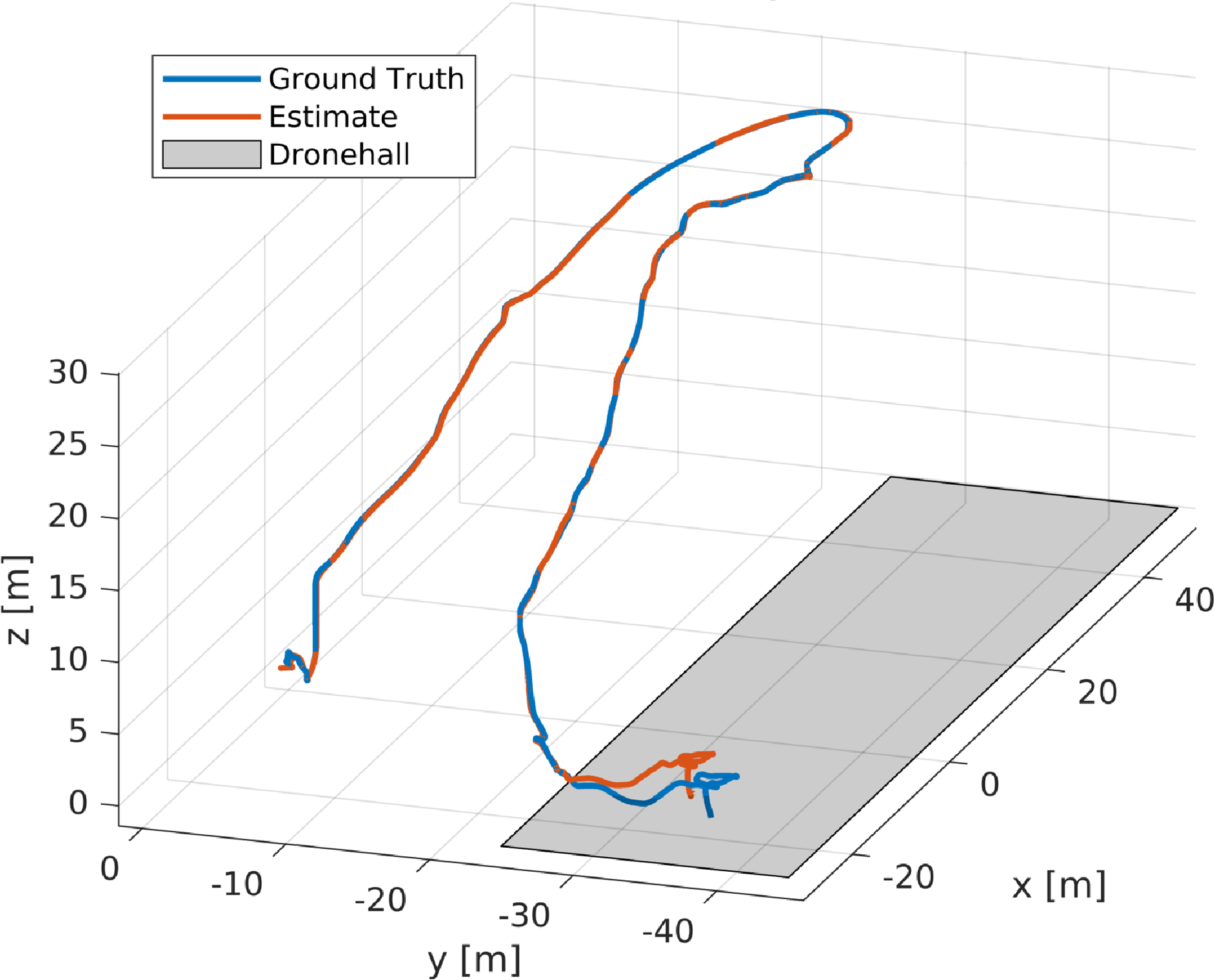

7.2. Usage and evaluation of example data with state-of-the-art VIO

As a validation of the usability of the datasets for VIO algorithm evaluation, raw IMU data as well as camera images from the Mars analog dataset 18 were used to run OpenVins Geneva et al. (2020), an open-source, state-of-the-art Multi-State Constrained Kalman Filter (MSCKF) based VIO framework. Figure 29 shows the estimated trajectory compared with RTK-GNSS-based ground truth. The estimated trajectory and ground truth are aligned along the four unobservable degrees of freedom of VIO, with the Umeyama alignment algorithm Umeyama (1991) computed over the full trajectory. The error of the estimate is calculated after the trajectory alignment and based on the absolute trajectory error (ATE) introduced by Zhang and Scaramuzza (2018). The absolute trajectory error of the position is 7.5 m, and the rotation error is 7°. It is important to note that this dataset poses particular challenges to vision-based algorithms. During the takeoff phase, the shadow of the platform with spinning propellers is in view of the navigation camera, resulting in moving features being tracked even though no motion is experienced by the platform itself. Moreover, during the flight, an almost featureless ground is seen from the camera, resulting in bad feature tracking (see the top left segment of Figure 29). Novel approaches as introduced by Hardt-Stremayr and Weiss (2020) are currently tackling this issue.

Figure 29.

Illustrative visual inertial localization example using a planar Mars analog dataset with state-of-the-art methods. The estimated trajectory in red in comparison to the provided ground truth of the dataset (blue). The estimated relative trajectory was globally aligned with the ground truth.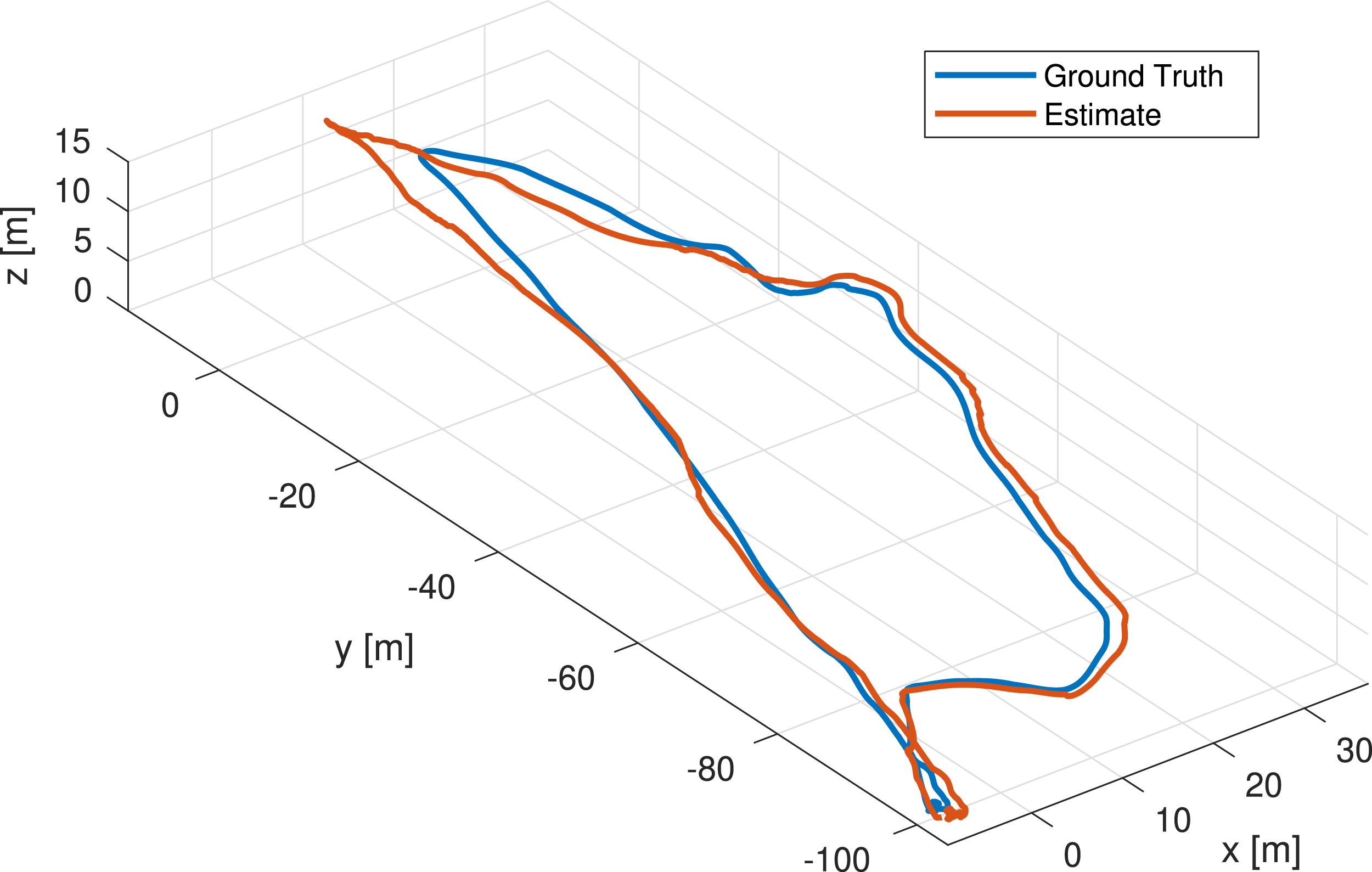

8. Lessons learned

This project posed challenges in terms of system and sensor setup as well as environmental difficulties. A few aspects have already been outlined in the System Setup Section 3. However, this section concludes the main difficulties that had to be overcome.

The generation of ground truth data posed multiple difficulties. First, the acquisition of highly accurate GNSS measurements was not straightforward because the vehicle hosts several computation boards as well as high-frequent data lines, which cause EMI. Thus, the electronic components and the GNSS antennas required customized shielding (see Figures 2 and 9) to reduce interfering signals to a level at which the GNSS provides position accuracy of 1 cm. Section 3.2.5 discusses this issue in detail. Another difficulty was the generation of continuous ground truth information for the outdoor to indoor transition area. This is due to RTK GNSS signals not being available close to the building area, and the motion capture system not covering the outside of the building entrance. Thus, a field of fiducial markers was used to provide ground truth for this transition area. This pose data is aligned with valid RTK GNSS data for the outdoor area and the motion capture reference frame via marker-object association. This method allows for global and local ground truth for each of the three segments of the outdoor-indoor transition trajectories.

Finally, the recording of high amounts of data, as done for this project, was a challenge. Special attention was given to the two onboard embedded platforms to reach balanced computational loads and, most importantly, the full use of available data interfaces. As shown by Figure 3, each board makes use of two storage entities with different data throughputs. USB3 interfaces also needed to be shared between storage devices and sensors. Thus, the data communication and recording needed to be designed to make use of the maximum data capacity that each interface and storage unit can provide. Overall, the system needed to write to an SD and SSD medium on each of the two embedded boards, thus requiring a total of four storage locations to record the data with the given measurement rate.

9. Conclusion and future work

This work introduced the INSANE dataset collection, which aims to provide multi-disciplinary in-flight data with a versatile sensor suite that is subject to real-world sensor effects. The flight scenarios address various research domains for vehicle localization. This work discussed individual aspects of the sensors and their integration in detail. The raw data for customized sensor calibrations and the analysis of specific sensor properties such as intrinsic, extrinsic and behavior for vibration behavior in a dedicated test bench setup are provided.

The quality of a dataset is directly correlated with the accuracy and uninterrupted availability of the accompanying ground truth information. Thus we presented a carefully designed setup to directly measure highly accurate ground truth as raw data. In contrast to other work, we do not need to filter this data to achieve the high accuracy, which prevents any filter-induced artifacts such as biases and inconsistencies.

Finally, we presented two show-cases which demonstrate the usability of the dataset with comparisons to the provided ground truth.

The lessons learned throughout this work are a crucial stepping stone for the development and extension of novel flight platforms. As for future aspects, it is planned to extend the dataset with new scenarios and sensor setups over time. Thus, the open-sourced dataset is not a static entity and will grow over time, following the same format for compatibility. Given the versatility of the presented setup, we believe that this data will enable researchers to develop and test future algorithms addressing real-world challenges in various disciplines.

Supplemental Material