Sage Journals: Discover world-class research

Abstract

A static world assumption is often used when considering the simultaneous localization and mapping (SLAM) problem. In reality, especially when long-term autonomy is the objective, this is not a valid assumption. This paper studies a scenario where landmarks can occupy multiple discrete positions at different points in time, where each possible position is added to a multi-hypothesis map representation. A selector-mixture distribution is introduced and used in the observation model. Each landmark position hypothesis is associated with one component in the mixture. The landmark movements are modeled by a discrete Markov chain and the Monte Carlo tree search algorithm is suggested to be used as component selector. The non-static environment model is further incorporated into the factor graph formulation of the SLAM problem and is solved by iterating between estimating discrete variables with a component selector and optimizing continuous variables with an efficient state-of-the-art nonlinear least squares SLAM solver. The proposed non-static SLAM system is validated in numerical simulation and with a publicly available dataset by showing that a non-static environment can successfully be navigated.

Keywords

Monte Carlo tree search non-static environment simultaneous localization and mapping multi-hypothesis

1. Introduction

In the field of robotics and autonomous driving, spacial awareness of the environment is crucial for the robot to safely and efficiently complete its task. For some applications the robot is given a, more or less precise, map of the operation area, constructed with some external dedicated mapping system (Artan et al., 2011). In other cases the robot is responsible of creating its own map while operating and at the same time localize itself within the map. This procedure is often referred to as simultatenous localization and mapping (SLAM). While both of these approaches have been successfully implemented, there are limitations in long-term operation since a static world assumption is often made. When life-long operation is the target, changes in the environment is inevitable and the problem of building adaptive maps has been mentioned as an important remaining challenge in this field (Cadena et al., 2016; Bresson et al., 2017).

Changes in an environment can be categorized into two main categories (Nielsen and Hendeby, 2022b):

• Dynamic changes, with objects moving relatively fast so that the perception of the object changes while the object is in field-of-view.

• Non-static changes (sometimes also referred to as semi-static changes (Rosen et al., 2016)), that are much slower and typically not captured by sensors in real time, but rather discovered when an area is revisited.

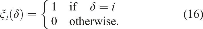
Dynamic changes are typically handled by filtering out measurements originating from moving objects (Hahnel et al., 2003; Wang et al., 2003), or in more sophisticated systems, track the moving obstacles (Dai et al., 2021; Wang et al., 2007). Either way, it is undesirable to update a more long-term map with these changes. This paper considers SLAM in an environment subject to non-static changes where landmarks move between different discrete positions. In the real world this has applications in indoor localization where objects such as furniture discretely change their positions, or doors are opened or closed. Also outdoor scenarios have possible applications where construction works can temporarily alter the environment or parking lots can be occupied or not. In Nielsen and Hendeby (2022b) it also described how this type of changes have high relevance in an underground mine environment, and it is shown that it is beneficial to somehow incorporate this type non-static changes into the SLAM model. This paper uses, the map representation presented in Nielsen and Hendeby (2022a), and further developed in Nielsen and Hendeby (2022b), where each landmark is modeled by discrete modes where only one can be true at each time instance. The movement of the landmarks are modeled by a discrete Markov chain.

The SLAM problem can be solved with Monte Carlo based methods such as FastSLAM 2.0 (Montemerlo et al., 2003), but in recent years optimization based SLAM solvers have become the de facto standard for solving SLAM problems (Agarwal et al., 2022; Kaess et al., 2012; Kümmerle et al., 2011). The problem is stated as factors in a graph, solved by optimizing the underlying nonlinear least squares problem. This paper introduces a selector-mixture distribution where only one of the components in a mixture is locally active. By using this distribution for landmark position representation, allowing different components to be active at different points in time, the Markov property in the landmark movements are combined with the modern graph-based SLAM framework. The optimization problem is by this approach divided into a discrete and a continuous part where the continuous part is solved by the graph-based SLAM solver, and the discrete part is optimized through component selection in the mixture distribution. A component selector operator based on the Monte Carlo tree search (MCTS) algorithm (Browne et al., 2012) is suggested and evaluated in experiments on real data. The properties of MCTS are shown to be beneficial for not getting stuck in local minima during the optimization process. The presented multi-hypotheses SLAM framework have the possibility to online provide both a position estimate and information about the current state of the environment. A prior map might be available or not, but the framework can in either case model changes of the environment not included in the map.

The main contributions of this paper are:

• The introduction of a selector-mixture distribution with the simplicity of a single Gaussian but with increased flexibility.

• Incorporation of the non-static environment model into the nonlinear least squares formulation of the SLAM problem.

• Introduction of MCTS as a selector strategy to solve the discrete part of the resulting non-static SLAM formulation.

• Validation of the proposed method on a publicly available dataset.

The paper is structured as follows. First, in Section 2 related work in literature is presented, then, the feature based multi-hypothesis SLAM problem is introduced in Section 3. The selector-mixture distribution is presented in Section 4 followed by suggestions on component selection strategies, where MCTS is one of them, in Section 5. Section 6 elaborates on effects of non-perfect sensors and negative information and how this can be included in the factor optimization, and Section 7 further discusses important implementation aspects. The proposed methods are evaluated in simulations and with real data in Section 8, and finally, concluding remarks are given in Section 9.

2. Related work

Long-term autonomy in SLAM applications have in the literature previously been addressed by introducing some sort of memory decay (Berrio et al., 2019b). In Rosen et al. (2016) landmark existence is estimated with a persistence filter, designed to run in parallel with a SLAM solver. Each landmark in the map has an associated probability of existence that decays over time according to a given model taking observations into account. In Nobre et al. (2018) the persistence filter is used but with the extension of modeling correlations between the landmarks. Also in Pitschl and Pryor (2019) a persistence model is used in an adaptive map maintenance technique. In Berrio et al. (2019a) each feature is scored as a function of times it has been observed. Low score features can then be disregarded not considered robust for localization.

Earlier works introducing multiple hypotheses more direct into factor graph representations have been developed mainly with the focus of handling uncertain data associations, for example, in (Chong, 2012). The adding of uncertain constraints in the factor graph are in (Latif et al., 2013) delayed until several new constraints agrees. They are then added as a batch of new constraints with a proposed algorithm called realizing, reversing, recovering (RRR). Others introduce a discrete variable in the factor graph to represent the uncertain data association, similar to the solution proposed in this paper where the discrete variable represents a position of a landmark. Various strategies have been proposed for solving such graphs. In Sünderhauf and Protzel (2012a, 2012b) switchable constraints are introduced where loop closure factors in practice can be activated or deactivated as part of the optimization process. A max-mixture distribution is introduced in Olson and Agarwal (2013) allowing for a more flexible representation of the measurement model. This is indeed a special case of the selector mixture proposed in this paper, but with the Markov property in the landmark movements the max-mixture representation has a risk of getting stuck in local minima. In Lu et al. (2021) discrete hypotheses modes represent ambiguities in observations. Each hypothesis is represented by a component in a Gaussian max-mixture model, and instead of a local search, consensus of pose hypotheses are used to re-initialize feature positions and guide the optimization towards global optimum. This works when the ambiguity is caused by observations not capturing all degrees of freedom in the landmark poses or similar-looking surroundings, but is incapable when landmarks are truly moved. The multi-hypothesis algorithm based on iSAM2 (MH-iSAM2) developed in (Hsiao and Kaess, 2019), is more general in the types of ambiguities that can be modeled but lacks the possibility to model the modes as a Markov chain.

In Segal and Reid (2014) a method based on message passing on a junction tree is presented. For the Gaussian case, this becomes equivalent to solving the factor graph based SLAM problem. In the presence of discrete variables, they provide an algorithm that iteratively estimates first the discrete variables then the continuous ones. This is in practice very similar to how the discrete variables are estimated in this paper. Also the work in Pfingsthorn and Birk (2013) is mixing discrete and continuous variables with discrete variables representing components in a mixture-distribution. However, they are focusing on observation ambiguities and the methods for finding the discrete variables do not model landmark movements. This iterative approach for solving the mixed discrete/continuous optimization problem for SLAM applications has recently been formalized and generalized in the method called discrete-continuous smoothing and mapping (DC-SAM) (Doherty et al., 2022). DC-SAM relies on that discrete variables conditioned on the continuous assignment admit a factorization into small subsets. These subsets can then be optimized separately with techniques suitable for that particular structure. This paper presents a method that is in spirit similar to DC-SAM, and the developed method could be fitted into the more general framework of DC-SAM as a special case to solve a specific structure of the discrete variables. Having a good initialization is important not to get stuck in local minima during the optimization. As pointed out in (Doherty et al., 2022), this is even more pronounced when mixing discrete and continuous variables, but the choice of method for optimizing the discrete variables also affects the risk of getting stuck in a local minimum.

The discrete part of the underlying optimization problem can be represented by an exponentially growing tree of hypotheses. This representation has similarities to how the data association problem is formulated and solved with the joint compatibility branch and bound (JCBB) method (Neira and Tardos 2001). JCBB exploits correlations between individual measurement innovations to efficiently search the hypotheses tree. In this paper, the features are allowed to move independently of each other and the problem is formulated such that the position of each feature can be treated separately. With that formulation of the optimization problem, JCBB is not directly applicable. To become applicable, the structure of the optimization problem would have to be rearranged, which, at least without further modifications, would make the method significantly more computationally expensive.

In our previous work multiple hypotheses in the map representation are introduced and the exponential growth in the number of hypotheses is limited by taking decisions based on statistical tests (Nielsen and Hendeby, 2022b). This however results in a somewhat overwhelming book-keeping of old hypotheses and a solution that does not scale well in the number of hypotheses since each hypothesis requires a dedicated SLAM solver. Here, the hypotheses are efficiently incorporated into the graph-based SLAM framework where modern nonlinear least-squares solvers can be utilized.

3. Feature based SLAM with non-static landmarks

The feature based SLAM problem can be defined as the joint inference of robot poses $X = {x_{t}}_{t = 1}^{T}$ , and poses of features in the map $M = {m_{j}}_{j = 1}^{K}$ , from a series of measurements Z. The trajectory length is defined by T and K is the total number of features. The measurements in Z consist of odometry Z_o = {z_t−1,t} and landmark observations $Z_{m} = {{Z_{t}^{i}}_{i = 1}^{k}}_{t = 1}^{T}$ , where i corresponds to a feature in the map m_i, and k is the number of features currently in field-of-view (FOV). Each $z_{t}^{i}$ denotes a relative pose measurement from x_t to m_i.

With a static world assumption the SLAM problem consists of estimating $p (X, M | Z)$ , which can be written as a product of the factor potentials in a factor graph (Dellaert and Kaess, 2017),

p (X, M | Z) \propto \prod_{i} p (z_{i} | X, M) .

(1)

Under an assumption of Gaussian noise models this can be formulated as a nonlinear least squares problem. Due to an inherently sparse structure, the problem can then be solved efficiently with specialized state-of-the-art solvers like g2o (Kümmerle et al., 2011), ceres (Agarwal et al., 2022), or the iSAM2 algorithm (Kaess et al., 2012) implemented in gtsam (Dellaert and GTSAM Contributors, 2022). They all use iterative solvers such as Gauss-Newton or Levenberg-Marquardt.

3.1. Multi-hypothesis map representation

This paper targets a non-static environment by allowing true feature positions to change between discrete positions modeled as multiple hypotheses. The feature based multi-hypothesis map representation from Nielsen and Hendeby (2022a) is in short defined by,

M = {[m_{1}^{s_{1}}, \dots, m_{n_{s_{1}}}^{s_{1}}, \dots, m_{1}^{s_{K}}, \dots, m_{n_{s_{K}}}^{s_{K}}]}^{⊤},

(2)

where s_j indicates which unique signature a specific landmark is associated with. All landmarks in

M

with the same signature represents the same real landmark but in different locations. That is, at each point in time, only one of the landmarks within a signature group is valid and observations are associated with that particular one. A hypothesis mode indicator vector is defined as

δ_{t} = {[δ_{t}^{1} \dots δ_{t}^{K}]}^{T},

(3)

where

δ_{t}^{j} = i

indicates that landmark

m_{i}^{s_{j}}

M

represents the current position of landmark j. A sequence of mode indicator vectors in time yields,

Δ = {δ_{0}, \dots, δ_{T}} .

(4)

3.2. Hypothesis Markov model

Assume the hypotheses are independent among different landmark groups, that is, landmarks change positions independently of each other, and that the transition between modes can be modeled by a Markov chain. Each mode indicator is distributed as, $δ_{t}^{j} \sim π_{t}^{j}$ , where $π_{t}^{j}$ can be represented as a column vector of discrete hypothesis weights. The distribution is recursively given by

π_{t}^{j} = A_{t}^{j} π_{t - 1}^{j},

(5)

where

A_{t}^{j}

is the Markov transition matrix possibly changing over time and for different landmark. The probability

p (δ_{t}^{j} = i)

i \in {1, \dots, n_{s_{j}}}

, is thus given by the ith element in

π_{t}^{j}

. To reduce the size of expressions, the notation

p (δ_{t}^{j})

is used for this probability when it applies to any possible i.

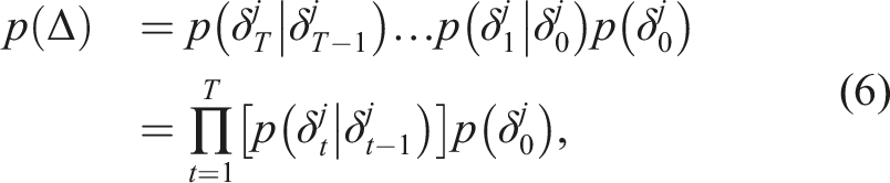
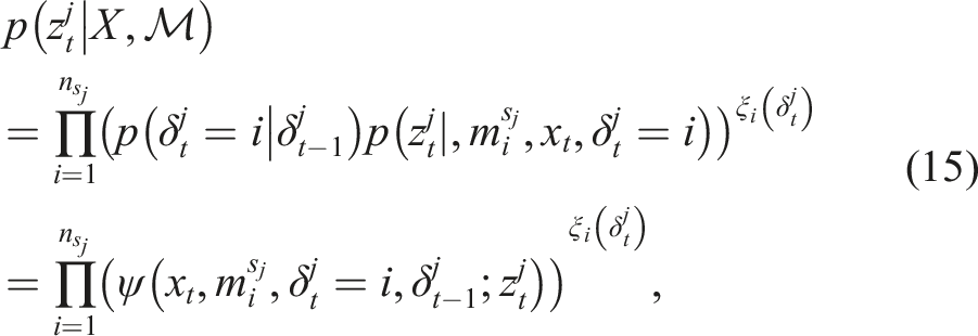
The joint probability of a sequence of hypothesis for a specific landmark can be formulated as

\begin{array}{l} p (Δ) & = p (δ_{T}^{j} | δ_{T - 1}^{j}) \dots p (δ_{1}^{j} | δ_{0}^{j}) p (δ_{0}^{j}) \\ = \prod_{t = 1}^{T} [p (δ_{t}^{j} | δ_{t - 1}^{j})] p (δ_{0}^{j}), \end{array}

(6)

where

p (δ_{t}^{j} | δ_{t - 1}^{j})

is given by the corresponding element in

A_{t}^{j}

3.3. Multi-hypothesis SLAM

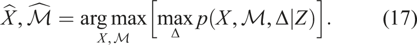
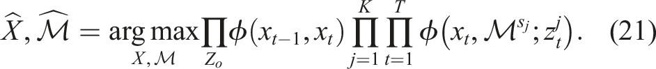
The MAP estimation of the multi-hypothesis SLAM problem can be formulated as,

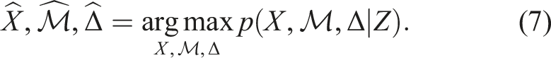
\hat{X}, \hat{M}, \hat{Δ} = \underset{X, M, Δ}{\arg \max} p (X, M, Δ | Z) .

(7)

Using Bayes rule and exploiting independence between X, $M$ , and Δ yields,

\hat{X}, \hat{M}, \hat{Δ} = \underset{X, M, Δ}{\arg \max} [p (X) p (M) p (Δ) p (Z | X, M, Δ)] .

(8)

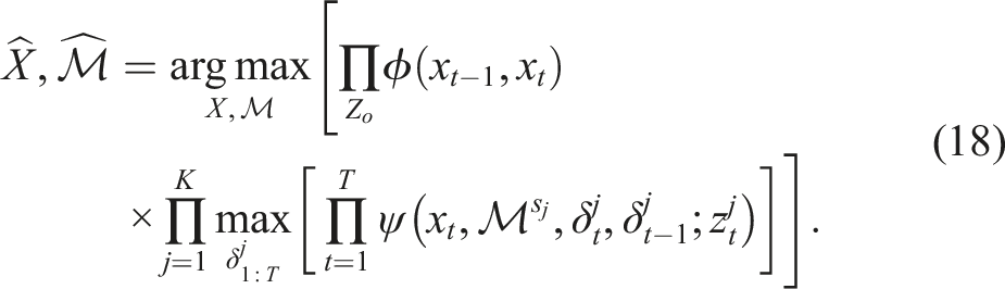
Assume measurements are independent and let ϕ(x_t−1, x_t) represent odometry factors not affected by the hypothesis choice. This gives,

\begin{array}{l} \hat{X}, \hat{M}, \hat{Δ} & = \underset{X, M, Δ}{\arg \max} [\prod_{Z_{o}} ϕ (x_{t - 1}, x_{t}) \\ \times [p (Δ) \prod_{j = 1}^{K} \prod_{t = 1}^{T} p (z_{t}^{j} | x_{t}, M^{s_{j}}, δ_{t}^{j})]], \end{array}

(9)

where uninformative priors are assumed and hence omitted. The set

M^{s_{j}}

are all landmark modes

m_{i}^{s_{j}}

i = 1, \dots, n_{s_{j}}

representing the same physical landmark.

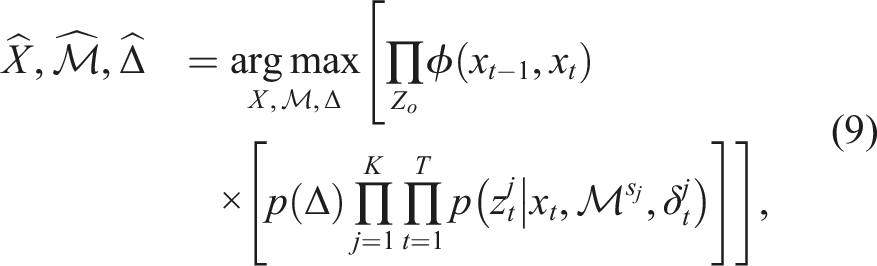
Due to mutual independence among the different landmark groups, the hypothesis probability can be moved inside the product over the landmarks. By also using (6), the MAP estimate can be factorized as

\begin{array}{l} \hat{X}, \hat{M}, \hat{Δ} & = \underset{X, M, Δ}{\arg \max} [\prod_{Z_{o}} ϕ (x_{t - 1}, x_{t}) \\ \times \prod_{j = 1}^{K} \prod_{t = 1}^{T} ψ (x_{t}, M^{s_{j}}, δ_{t}^{j}, δ_{t - 1}^{j}; z_{t}^{j})], \end{array}

(10)

with

ψ (x_{t}, M^{s_{j}}, δ_{t}^{j}, δ_{t - 1}^{j}; z_{t}^{j}) = p (δ_{t}^{j} | δ_{t - 1}^{j}) p (z_{t}^{j} | x_{t}, M^{s_{j}}, δ_{t}^{j}),

(11)

where the notation

ψ (x_{t}, M^{s_{j}}, δ_{t}^{j}, δ_{t - 1}^{j}; z_{t}^{j})

indicates that this is a function of x_t,

M^{s_{j}}

δ_{t}^{j}

, and

δ_{t - 1}^{j}

, with

z_{t}^{j}

given.

3.4. Hypotheses in a factor graph

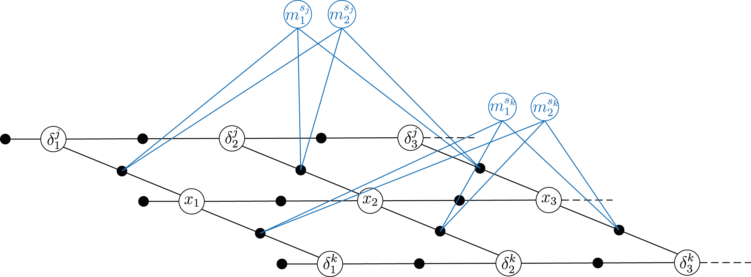
The mode indicators, as defined in (3), can be added as discrete variables in a factor graph. The factor graph for one landmark with two possible modes, observed from three consecutive states is presented in Figure 1. Each factor ϕ(·) in the graph represents a factor in the MAP estimate (10). The factor nodes $ϕ (δ_{1}^{j})$ and $ϕ (x_{1}, m_{1}^{s_{j}}, m_{2}^{s_{j}}, δ_{1}^{j})$ together form $ψ (x_{1}, M^{s_{j}}, δ_{1}^{j}, δ_{0}^{j}; z_{1}^{j})$ as given in (11), and

ψ (x_{2}, M^{s_{j}}, δ_{2}^{j}, δ_{1}^{j}; z_{2}^{j}) = ϕ (δ_{1}^{j}, δ_{2}^{j}) ϕ (x_{2}, m_{1}^{s_{j}}, m_{2}^{s_{j}}, δ_{2}^{j})

(12)

and so on. Figure 2 depicts how the graph extends when another landmark with two possible modes is present.

Figure 1.

Factor graph for three consecutive states where one landmark with two possible modes is observed in each state.

Figure 2.

Factor graph for three consecutive states where two landmarks with two possible modes are observed in each state. Each filled black dot represents one factor.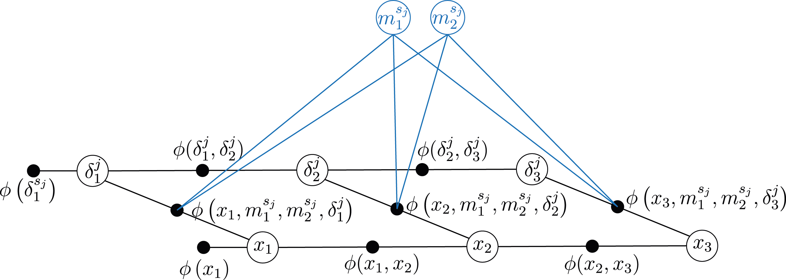

There are two issues with the factor graph formulation of the MAP inference in (10) that must be addressed. First, state-of-the-art graph-SLAM solvers cannot efficiently combine discrete and continuous variables (Sünderhauf and Protzel, 2012b). In Segal and Reid (2014) a method based on message passing in a junction tree is presented to handle uncertain loop closures. In the presence of discrete variables, they provide an iterative algorithm that first estimates the discrete variables then optimize continuous ones. This strategy is adopted in this paper and is further described in Section 5. Second, the Markov property on the feature dynamics prevents each mode indicator to be independently estimated without risking to get stuck in local minima and obtain sub-optimal solutions. This problem is addressed by introducing a selector-mixture distribution. By describing the measurement likelihoods as such distributions, the estimation of discrete values modeled by a Markov chain can be mathematically described.

4. Selector-mixture distribution

In Olson and Agarwal (2013), the max-mixture distribution is introduced as a way to represent multiple hypotheses within the SLAM framework. Unlike the sum-mixture, commonly used to represent multi-modal distributions, the max-mixture is suitable for optimization in least-square graph based SLAM applications. A sum-mixture might also give infeasible results in “either-or” situations, whereas selecting only one out of many components will always provide a feasible solution. The weighted mean of a number of feasible robot positions might end up, for example, inside a wall. It might be better to update the position with the “wrong” hypothesis and later switch when you know better, than to obtain a weighted mean that was never valid. However, the max-mixture only gives locally optimal solutions and with a Markov property present, it is even more important to not get stuck in a local minima at an early stage. This section introduces a generalization of the max-mixture distribution, the selector-mixture distribution.

Consider a mixture of Gaussian components, where only one component in the mixture is selected given some criterion specified by a general component selector operator, σ_k(·). This is a unary operator and applied on the factors in the factor graph yields,

p (z_{i} | X, M) = σ_{k} ({w_{j} N (z_{i}; μ_{j}, Ω_{j})}) .

(13)

Using the max-operator as the component selector operator would result in a max-mixture,

p (z_{i} | X, M) = \max_{j} {w_{j} N (z_{i}; μ_{j}, Ω_{j})},

(14)

and hence the max-mixture is a special case of a selector-mixture.

Figure 3 shows how a multi-modal distribution would be represented by a sum-mixture and a max-mixture. The discontinuity in the derivative that appears in the intersection points in the max-mixture will appear with any component selector operator and is solved by locally using only the selected component. As a consequence, only local optimality is obtained and good initial values are important.

Figure 3.

Conceptual comparison of sum-mixture and max-mixture distributions.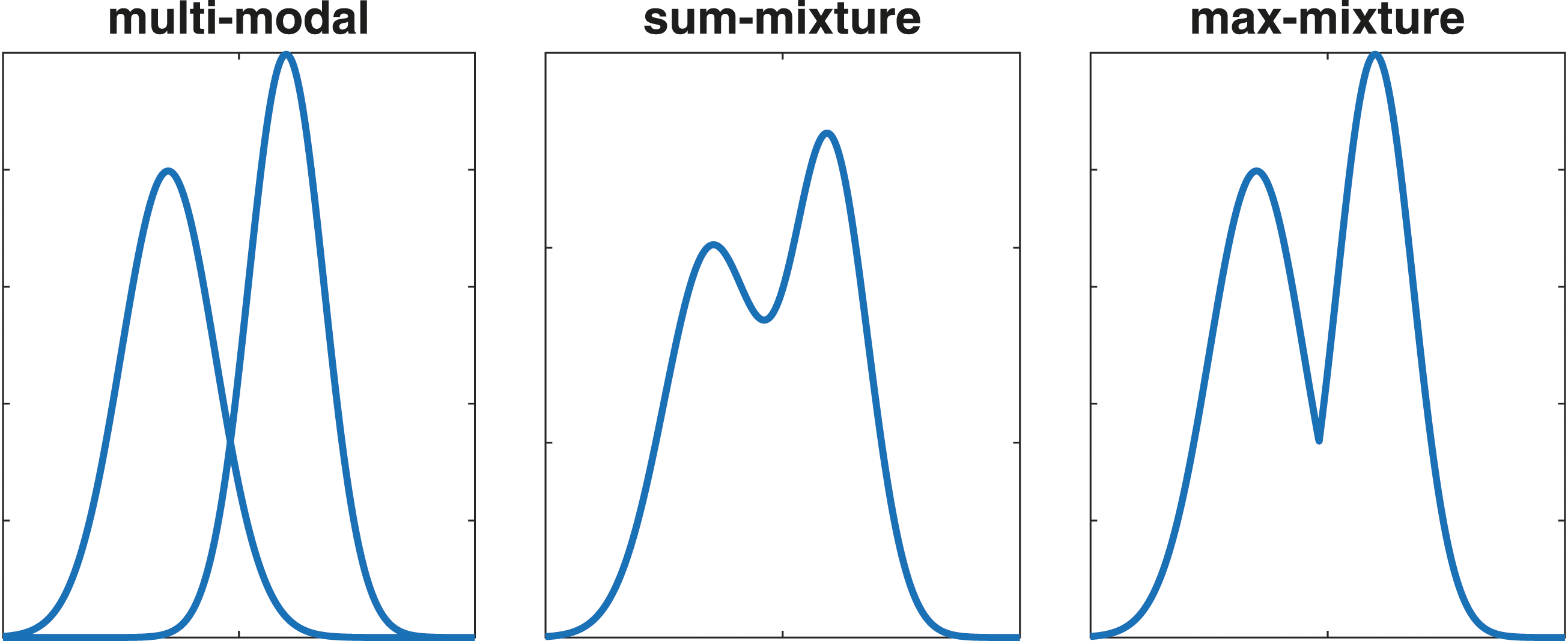

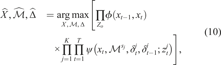
However, the generalized selector criterion allows for incorporating the Markov model of the landmark movements into the mixture. Considering the multi-mode formulation where each component in the mixture originates from one mode of a landmark, the selector mixture can be expressed as,

\begin{array}{l} p (z_{t}^{j} | X, M) \\ = \prod_{i = 1}^{n_{s_{j}}} (p (δ_{t}^{j} = {i | δ_{t - 1}^{j}) p (z_{t}^{j} |, m_{i}^{s_{j}}, x_{t}, δ_{t}^{j} = i))}^{ξ_{i} (δ_{t}^{j})} \\ = {\prod_{i = 1}^{n_{s_{j}}} (ψ (x_{t}, m_{i}^{s_{j}}, δ_{t}^{j} = i, δ_{t - 1}^{j}; z_{t}^{j}))}^{ξ_{i} (δ_{t}^{j})}, \end{array}

(15)

where

ξ_{i} (δ) = {\begin{cases} 1 if δ = i \\ 0 otherwise . \end{cases}

(16)

The responsibility of the selector operator boils down to selecting a sequence of mode indicators for each landmark. Next section gives the criterion for how to perform such selection in the feature based SLAM problem.

For a mixture to be a proper distribution it has to integrate to one. For the sum-mixture this is achieved with the constraint that the component weights should sum to one, but for selector-mixtures normalization is in general more difficult to achieve. However, as argued in Olson and Agarwal (2013), the normalization constant has no effect in the ML inference and is therefore unnecessary to compute in this application.

5. SLAM with component selector

This section formulates the SLAM problem with selector-mixture distributions in the observation model. The criterion for selection is derived and the component selectors evaluated in this paper is presented.

5.1. Mixture SLAM

With the max-product algorithm (Abdi and Ristaniemi 2020), the MAP problem (7) can be rewritten as,

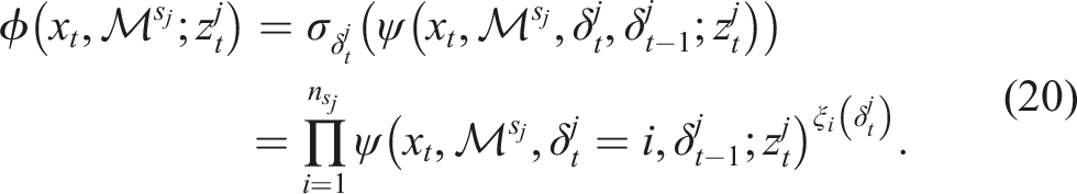
\hat{X}, \hat{M} = \underset{X, M}{\arg \max} [\max_{Δ} p (X, M, Δ | Z)] .

(17)

Following the steps in Section 3.3 yields,

\begin{array}{l} \hat{X}, \hat{M} = \underset{X, M}{\arg \max} [\prod_{Z_{o}} ϕ (x_{t - 1}, x_{t}) \\ \times \prod_{j = 1}^{K} \max_{δ_{1 : T}^{j}} [\prod_{t = 1}^{T} ψ (x_{t}, M^{s_{j}}, δ_{t}^{j}, δ_{t - 1}^{j}; z_{t}^{j})]] . \end{array}

(18)

The selector problem is to find the mode indicator sequence by solving

\max_{δ_{1 : T}^{j}} [\prod_{t = 1}^{T} ψ (x_{t}, M^{s_{j}}, δ_{t}^{j}, δ_{t - 1}^{j}; z_{t}^{j})]

(19)

in an efficient way. Ignoring the Markov model

p (δ_{t}^{j} | δ_{t - 1}^{j})

, and selecting the most probable mode given the observation, results in the max-mixture method where the max-operator can be moved inside the product. This is indeed done in (Li et al., 2021) for observation ambiguities, but then with the prerequisite that the

δ_{t}^{j}

are truly mutually independent conditioned on x_t and

M^{s_{j}}

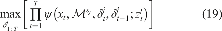
Formulated with a selector-mixture with a component selector operator $σ_{δ_{t}^{j}}$ defined with (19) as the selection criterion, factors for the observation likelihoods yields,

\begin{array}{l} ϕ (x_{t}, M^{s_{j}}; z_{t}^{j}) = σ_{δ_{t}^{j}} (ψ (x_{t}, M^{s_{j}}, δ_{t}^{j}, δ_{t - 1}^{j}; z_{t}^{j})) \\ = \prod_{i = 1}^{n_{s_{j}}} ψ {(x_{t}, M^{s_{j}}, δ_{t}^{j} = i, δ_{t - 1}^{j}; z_{t}^{j})}^{ξ_{i} (δ_{t}^{j})} . \end{array}

(20)

Finally, the MAP problem can be written as separate factors,

\hat{X}, \hat{M} = \underset{X, M}{\arg \max} \prod_{Z_{o}} ϕ (x_{t - 1}, x_{t}) \prod_{j = 1}^{K} \prod_{t = 1}^{T} ϕ (x_{t}, M^{s_{j}}; z_{t}^{j}) .

(21)

Solving (19) is by no means trivial and typically it also must be done in, at least close to, real time. A presentation of three different component selectors evaluated in this paper now follows. First, a naive nearest neighbor (NN) approach is introduced, completely neglecting the Markov property in the modes, in essence this is the max-mixture approach but with an added iterative re-linearization and with utilization of negative information. This selector is mostly included as a reference. Then, a variant based on ideas from the expectation maximization (EM) algorithm is presented. This approach provides a natural way of separating the optimization of the discrete and continuous variables in the factor graph that is adopted also for the other component selectors. The last version of a component selector utilizes Monte Carlo Tree Search (MCTS), which with the inherent randomness mitigates the risk of getting stuck in local minima.

5.2. NN as component selector

A component selector neglecting the Markov property in the mode switches can be constructed through an NN approach. The component with the maximum observation likelihood is selected locally in each time instance,

\underset{i}{\arg \max} p (z_{t}^{j} | m_{i}^{s_{j}}, x_{t}, δ_{t}^{j} = i) .

(22)

This component selector might perform poorly in noisy, heavy cluttered scenarios, where the selector will jump back and forth between modes based on single observations. So far, this is exactly equal to the max-mixture method presented in Olson and Agarwal (2013). However, the NN method used in the experiments section is boosted with the iterative re-linearization described in the next section and with utilization of negative information obtained from the probability of detection of each landmark, see section 6.

5.3. EM as component selector

The EM algorithm is an ML approach to get an estimate of a parameter X given some observations Z and hidden variables θ. The complete-data likelihood p(Z, θ|X) is inaccessible due to the hidden variable and knowledge about the latent variables in θ is only given through the posterior distribution p(θ|Z, X). The EM algorithm consists of iterating between two steps:

1. The E-step, where the expected value of the hidden variable θ is taken given an initial value of X, and,

2. the M-step, where the ML estimate of X is obtained given the expected value of θ.

The iteration are continued until convergence, according to some criterion (Bishop, 2006).

This iterative approach is in practice similar to what is described in (Segal and Reid, 2014) for discrete/continuous variable optimization in junction trees. Applied to the mixture SLAM problem described in (21) the sequence of mode indicator vectors $δ_{1 : T}^{j}$ can be considered the hidden variables and the state X and map of landmark poses $M$ are the parameters to estimate. The posterior distribution for each $δ_{t}^{j}$ is given by

p (δ_{t}^{j} | Z, X) = \frac{p (Z | δ_{t}^{j}, X, M) p (δ_{t}^{j})}{\sum_{δ_{t}^{j}} p (δ_{t}^{j}) p (Z | δ_{t}^{j}, X, M)},

(23)

where it is utilized that the mode is independent of the state and map,

p (δ_{t}^{j} | X, M) = p (δ_{t}^{j})

. The prior

p (δ_{t}^{j})

for each t is given by the Markov chain described in (5) given

p (δ_{1}^{j})

. For each posterior distribution

p (δ_{t}^{j} | Z, X)

the most probable value of

δ_{t}^{j}

is selected to perform the maximization in (19).

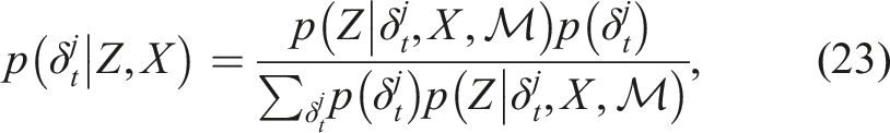
Taking the expected value of a discrete random variable (23) in general gives a non-integer value, resulting in an undefined mode selection. Also, the expected value assumes the discrete variable are in some sense ordered. A value closer to the expected value should be more likely than a value far away, which is not the case for the feature position hypotheses. They are given a number just for identification. Instead the “winner take all”-variant of the EM algorithm as described in (Neal and Hinton, 1998) is used. That is, the mode that maximizes (23) with X and $M$ fixed, is used in the M-step. The M-step constitutes running one optimization step with the least-squares optimizer to get a new estimate of X and $M$ given the sequences of mode values. This iterative re-linearization approach is adopted for all component selectors in this paper, and reduces the risk of getting stuck in local minima.

This procedure is in practice similar to what is described as the outer EM loop in (Pfeifer and Protzel, 2019), where the EM-algorithm is computed only once per time step. Here, the EM-algorithm is iterated until the mode vector does not change, but since no actual expectation is taken in the E-step, the convergence guarantees of the original EM-algorithm is lost and convergence has to be achieved over time. In Pfeifer and Protzel (2019) it is discussed and also shown in experiments that for SLAM and localization problems it is in practice possible to attain convergence. The main argument is that the algorithm is solved iteratively, and every time step starts close to the minimum that the previous one found. Still, there is always a risk, due to the structure and nonlinearity in a particular estimation problem, to get stuck in a local minimum.

5.4. MCTS as component selector

MCTS is a stochastic search algorithm for finding optimal actions in decision processes. This algorithm is often used in combination with deep neural nets to train autonomous agents to play complex games (Silver et al., 2016; Schrittwieser et al., 2020). A search tree is iteratively built, guided by results from previous explorations of the tree, until a predefined computational budget is reached. Four steps are executed in each iteration; selection, expansion, simulation, and backpropagation (Browne et al., 2012). See Figure 4 for an illustration of the MCTS algorithm. The steps are realized by two policies:

1. Tree policy: Selects an existing node and expand it with a new leaf.

2. Rollout policy: Performs a play-out (simulation) from a given node to produce a value estimate which is some kind of measure of the expected future performance.

Figure 4.

Overview of the MCTS algorithm. Figure from (Boström-Rost et al., 2021).

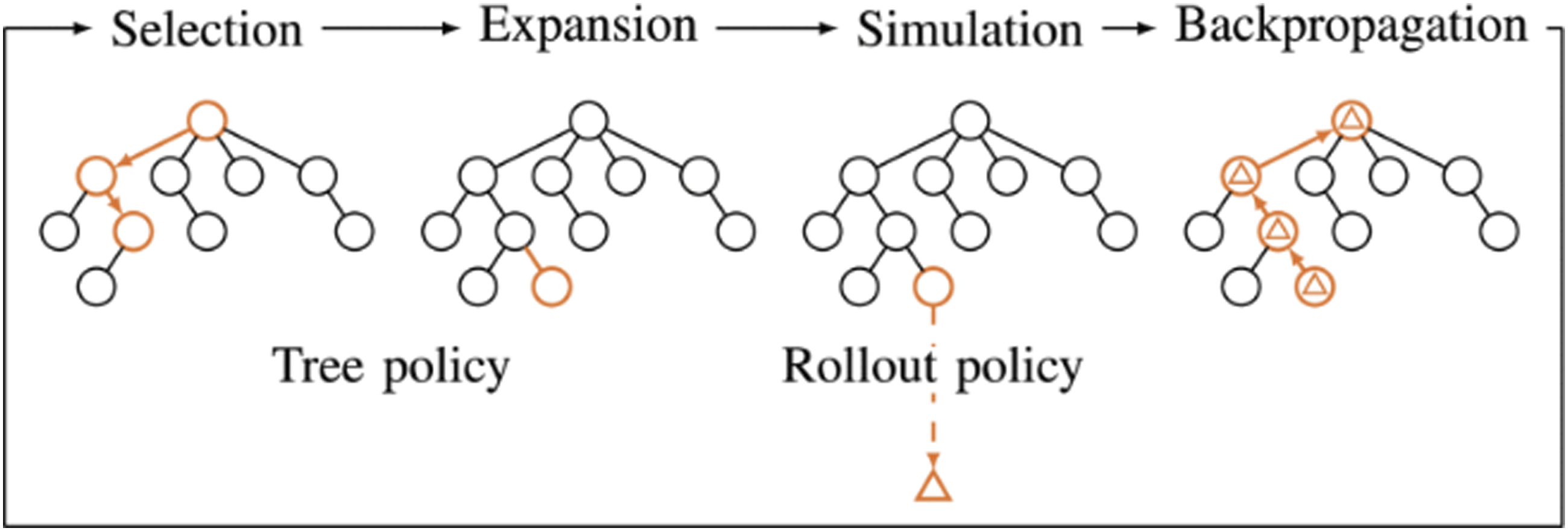
The estimated value is used to update node statistics in the backpropagation step for visited nodes all the way back to the root.

Given a prior $p (δ_{1}^{j})$ such a tree can be built for each $δ_{1 : t}^{j}$ to obtain the sequence of mode vectors that approximates the maximization in (19). Each node i in the tree holds information about the number of visits so far n_i, the corresponding mode indicator value $δ_{t}^{j}$ , and the estimated value of being in that particular node, Q_i. The value Q_i is here defined by the average total log-likelihood of mode sequences passing through that node,

Q_{i} = \frac{1}{n_{i}} \sum_{k = 1}^{n_{i}} p (δ_{1 : t, k}^{j} | Z, X),

(24)

where each

δ_{1 : t, k}^{j}

is one mode sequence obtained from the policies.

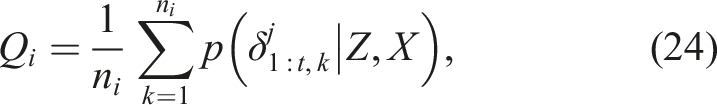
The tree policy used to select a node for expansion is implemented by the upper confidence bound for trees (UCT) policy (Kocsis and Szepesvári, 2006). Starting at the root node, a child is selected and the tree traversed until a node is reached that has unvisited children. A child i is selected according to,

\underset{i}{\arg \max} [Q_{i} + C_{p} \sqrt{\frac{\ln n}{n_{i}}}],

(25)

where n is the number of visits of the parent node and C_p > 0 is a parameter for the exploration-exploitation trade-off in the tree. In the UCT policy, the values of Q_i are understood to be in the interval [0,1] (Kocsis and Szepesvári, 2006). For this environment the log-likelihoods constituting Q_i can be in the interval

(- \infty, 0]

. In (Schadd et al., 2008) they suggest re-scaling the values by domain specific knowledge about maximum/minimum values. This is not possible since the log-likelihood can attain infinitely large negative values. Instead the normalization methods suggested in Schrittwieser et al. (2020) are used. When a node is reached during the selection stage, a normalized

{\bar{Q}}_{i}

value, to be used in the UCT policy, is computed given the tree so far,

{\bar{Q}}_{i} = \frac{Q_{i} - \min_{j \in t r e e} Q_{j}}{\max_{j \in t r e e} Q_{j} - \min_{j \in t r e e} Q_{j}}

(26)

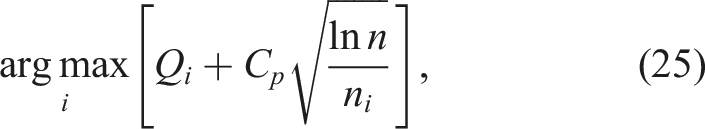
When the computational budget is reached, the child with highest visit count is selected as next mode (Browne et al., 2012). The iterative approach of estimating the discrete mode indicators followed by optimizing variables, is adopted also with this component selector.

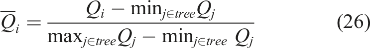
For the experiments conducted in this paper, the parallel MCTS algorithm in Chaslot et al. (2008) implemented in Strandmark (2020), is used as a base, but has been modified with the normalization in (26).

6. Non-perfect sensors and negative information

In practice, sensors and feature extraction methods are never perfect. Features/landmarks that should have been observed is not, and false positives might occur in the data. In target tracking theory this is modeled by a probability of detection, P_D, and a false alarm distribution (Bar-Shalom et al., 2011). In the presented multi-hypothesis SLAM framework a false alarm will result in a new hypothesis that anyway soon will become very unlikely. The probability of detection is in target tracking often chosen as a constant determined by the sensor and feature extraction method. However, introducing P_D as a function of landmarks and robot positions, into the SLAM problem allows utilizing negative information into the factor graph.

6.1. Probability of detection

Considering non-perfect feature detectors, the likelihood of an observation is the likelihood obtained from the selected Gaussian component multiplied by $P_{D} (x_{t}, m_{i}^{s_{j}})$ , which is the probability of detecting $m_{i}^{s_{j}}$ from the position x_t. The expression in (11) thus becomes,

\begin{array}{l} ψ (x_{t}, {m^{s_{j}}}, δ_{t}^{j}, δ_{t - 1}^{j}) = \\ p (δ_{t}^{j} | δ_{t - 1}^{j}) P_{D} (x_{t}, m_{i}^{s_{j}}) p (z_{t}^{j} | x_{t}, {m^{s_{j}}}, δ_{t}^{j}), \end{array}

(27)

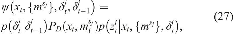
6.2. Negative information as a factor

To utilize negative information, the factors connected to landmark observations (20) can be written as

\begin{array}{l} ϕ (x_{t}, {m^{s_{j}}}; z_{t}^{j}) = \\ {\begin{cases} \prod_{i = 1}^{n_{s_{j}}} ψ {(x_{t}, {m^{s_{j}}}, δ_{t}^{j} = i, δ_{t - 1}^{j})}^{ξ_{i} (δ_{t}^{j})} & if z_{t}^{j} \neq \emptyset \\ \prod_{i = 1}^{n_{s_{j}}} {(1 - P_{D} (x_{t}, m_{i}^{s_{j}}))}^{ξ_{i} (δ_{t}^{j})} & if z_{t}^{j} = \emptyset, \end{cases} \end{array}

(28)

where

z_{t}^{j} = \emptyset

indicates no observation available. Landmarks far away from FOV will have a probability of detection close to zero, resulting in an approximately constant factor with value 1. Such factors will not contribute in the optimization and for landmarks with a probability of detection below a threshold,

P_{D} (x_{t}, m_{i}^{s_{j}}) < γ

, this factor can be omitted.

7. Implementation aspects

This section contains practical considerations for implementation of the proposed selector-mixture SLAM formulation and associated component selectors. It is explained how new feature modes are created and how the probability of a landmark being in FOV can be computed. Methods suggested here are not the only options and suitable methods may vary between different applications and requirements. However, this is how the evaluation in the experiment section is implemented.

7.1. Gating and mode creation

Incoming observations will not match the known position if a landmark has moved, and a new mode of a landmark is created if a measurement does not gate with any known mode. The gating is performed through a Mahalanobis distance based on the projected estimation uncertainty, similar to the individual compatibility (IC) matching technique for data association (Kaess and Dellaert, 2009).

A predicted measurement is given by the measurement model,

z_{t}^{j} = h_{i} (x_{t}, m_{i}^{s_{j}}) + v,

(29)

where v is additive zero mean Gaussian noise with covariance Γ, assumed equal for all landmarks. The nonlinear least-squares solver provides a current state estimate in form of a normal distribution, with mean

{[{\hat{x}}_{t}, \hat{M}]}^{⊤}

and covariance Σ. A square Mahalanobis distance function follows a chi-square distribution, and a chi-square test is used for gating,

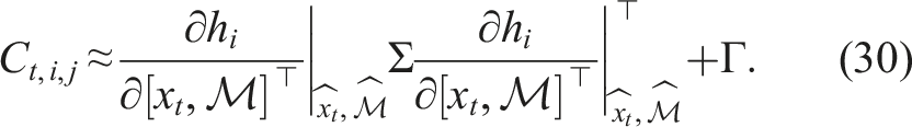
where d is the dimension of the measurement and α is the desired confidence level. The projected uncertainty is approximated through (Kaess and Dellaert, 2009),

C_{t, i, j} \approx {\frac{\partial h_{i}}{\partial {[x_{t}, M]}^{⊤}} |}_{{\hat{x}}_{t}, \hat{M}} Σ {\frac{\partial h_{i}}{\partial {[x_{t}, M]}^{⊤}} |}_{{\hat{x}}_{t}, \hat{M}}^{⊤} + Γ .

(30)

The confidence level α is a tuning parameter that should be small enough for hypotheses to be created for small landmark movements, but still high enough to not trigger hypotheses caused by measurement noise.

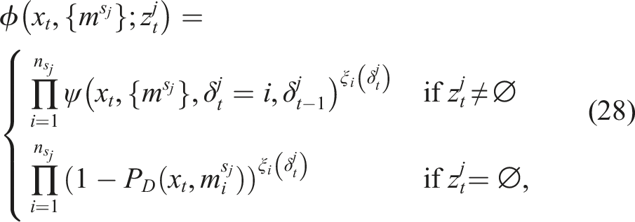
7.2. Negative information and probability of detection

For negative information representation, the factor in (28) is used. In theory, this would require a well defined Jacobian of the function. However, by only using the missed detection information in the estimation of the discrete mode selectors, and only utilizing actual measurements in the nonlinear least square optimization, this is in practice not needed. This practicality is indeed an approximation, but it significantly reduces the complexity in the optimization since many of the factors can be omitted.

The probability of detection P_D(x, m) is modeled by a constant factor and a function depending on the FOV sector,

P_{D} (x, m) = P_{D} P_{FOV} (x, m) .

(31)

The probability of FOV function, P_FOV(x, m), is approximated by modeling predicted range r, and bearing b, as Gaussian distributions according to (29) and then estimated by P_FOV(x, m) ≈ P(r < γ_r)P(|b| < γ_b).

8. Experiments and results

The evaluation of the proposed multi-hypothesis SLAM formulation has two objectives; compare the different component selectors and elaborate about their pros and cons, and verify the usefulness of creating and maintaining multiple hypotheses by successfully navigating a non-static environment. Due to the lack of datasets with naturally occurring non-static changes, the procedure of imposing changes of varying degree, as done in Nobre et al. (2018), is used. The performance of the suggested method is assessed through a 2D SLAM system in which odometry and range and bearing measurements are added to a factor graph, and the iSAM2 (Kaess et al., 2012) solver, implemented by modifications of gt-sam (Dellaert and GTSAM Contributors, 2022), is used to solve the nonlinear least squares problem. The modifications mainly constitute changes in the bookkeeping of variables and factors, to allow for a factor to switch its dependency to a different variable according to the mode indicator.

First, the component selectors are compared in a simulated experiment where the performance of the actual selector is isolated from other affecting properties occurring in a complex system. Then, the complete system is evaluated on a real dataset, where it is also compared to the max-mixture algorithm.

8.1. Simulated selector comparison

In a simulated open environment, a robot is placed at the origo and landmark measurements are simulated as x, y-coordinates with added white Gaussian noise, $N (0, R)$ . Three different positions of the landmark is used and 10 consecutive measurements are simulated from each mode before the landmark is “moved” to the next mode, see Figure 5. In Figure 6 the number of wrongly selected modes for the different selectors are presented for increasing measurement noise, R = rI, where I is identity. With a larger measurement noise, it is clear that the utilization of the Markov property in the mode sequence causes the EM and MCTS selectors to outperform the NN.

Figure 5.

The robot is placed at origo and measurements are simulated for three possible modes of one particular landmark, each represented by green, purple, or yellow color. The measurements originating from a landmark mode is marked with crosses of the same color. This particular realization is done with the measurement noise level r = 0.2.

Figure 6.

For different measurement noises, the average ratio of wrong mode selections during the total 30 timesteps are estimated with 100 MC realizations.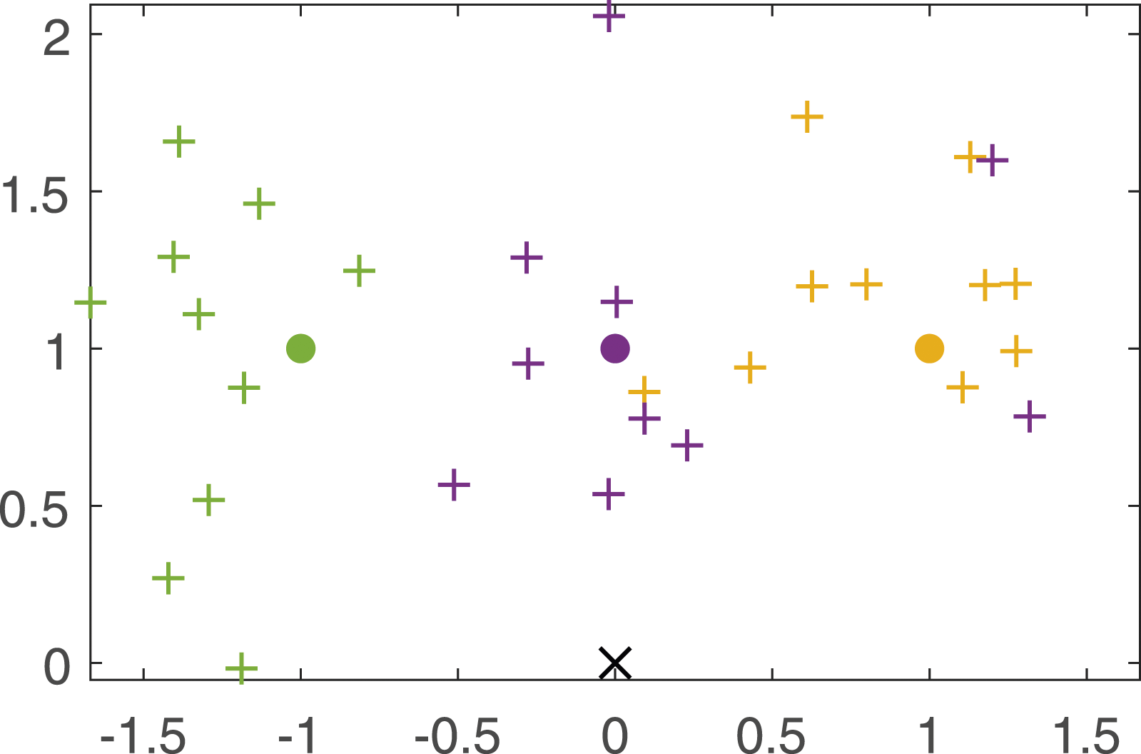

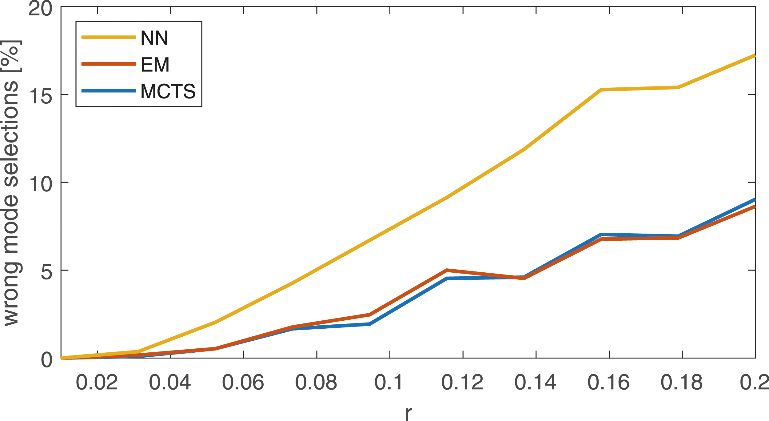
Figure 7 show the performance of the same scenario but with a complete SLAM solver executed. The Cartesian x, y coordinates together with the heading, constitutes the 2D state vector and a process noise of Q = diag(0.01², 0.01², 0.001²), is used. It is clear that the erroneous data associations that the wrongly selected modes caused with the NN selector, degrades the accuracy in the position estimates.

Figure 7.

Combined RMSE of the final robot position and final landmark position after all measurements have been processed. 100 MC realizations for each r, R = diag(r, r).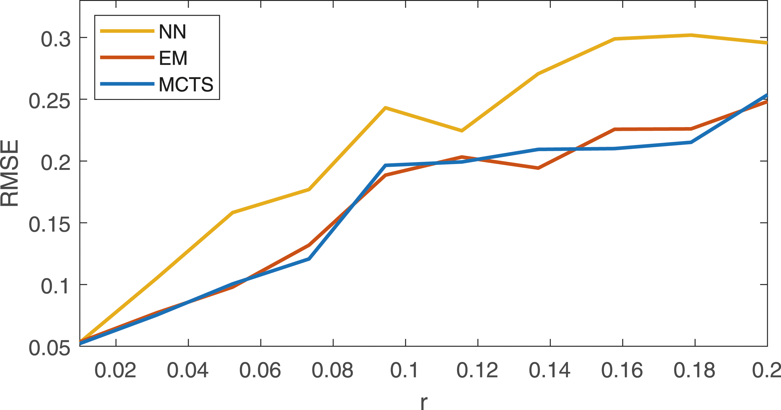

8.2. Real data experiment

This section contains experiments on recorded data.

8.2.1. The dataset

The UTIAS dataset (Leung et al., 2011) is used for validation. The dataset consists of odometry and range/bearing observations of 2D point features, and comes with ground-truth trajectories with accuracy in the order of 1 mm. The landmarks are visually detected, and each landmark is uniquely identified with a barcode. Since there are no non-static landmarks in the dataset, changes are imposed as proposed in (Nobre et al., 2018), that is, landmarks likely to have correlated position are identified and then moved together as a group in incremental steps in the x-direction. In each execution, the SLAM solver is initially given landmark positions according to the ground truth, plus possible delta change in the x-direction, with provided uncertainty. The result is evaluated as root mean square error (RMSE) towards the ground truth trajectory and landmark positions. The dataset includes a number of setups and runs where the three first are used for evaluation in this paper. Figure 8 shows the ground truth data for these three dataset and depicts the moved landmarks in each of them.

Figure 8.

Ground truth (GT) trajectories for three of the datasets together with estimated trajectories with the MCTS method and max-mixture method. Filled circles marks the landmarks and the orange are moved with varying distance in the x-direction. A cross marks the start of the trajectory. For dataset 1 and 3, the trajectories are created with a delta displacement of 1.0 m and for dataset 2 with 2.1 m. In dataset 2 the red part of the trajectory is of special interest since there is a long period without landmarks in field-of-view.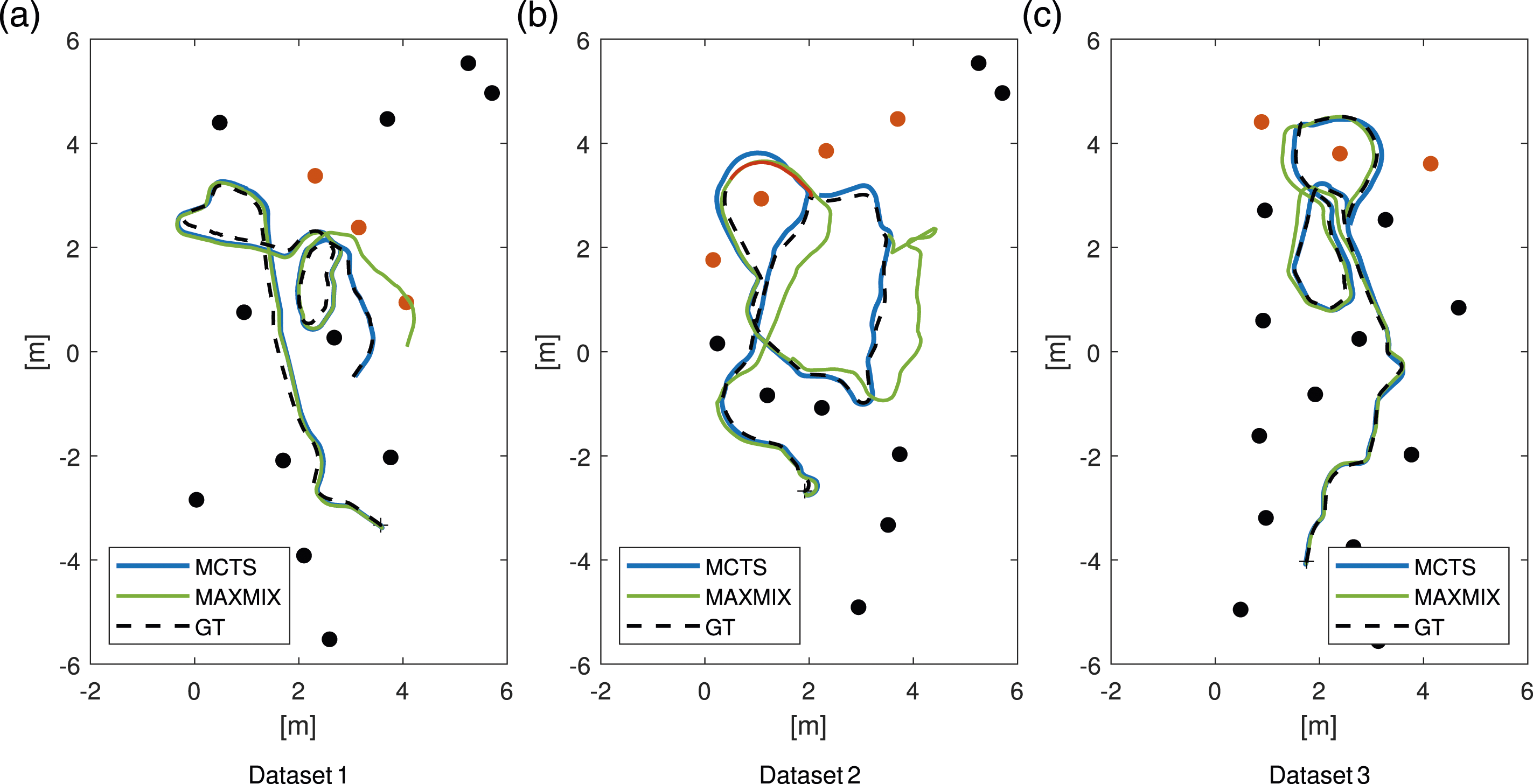

By inspection of the ground truth data and the measurement it is seen that the measurement noise is not uniform within the sensors FOV for this dataset, especially not close to the borders of FOV. Therefore, all measurement with ranges exceeding 5 m and with bearing outside ± 0.4 rad are disregarded. The odometry is sampled with d_t = 0.02 s and the process noise for the odometry is set to $Q = d_{t}^{2} {0.01}^{2} I$ , where I is identity, with the motion model according to the between-factor in gtsam (Dellaert and GTSAM Contributors, 2022).

The proposed component selection method is compared to the max-mixture method presented in (Olson and Agarwal, 2013). Existing implementations of this method are focused on the odometry factors and ambiguous loop-closures. Therefore, our own implementation is used for the max-mixture method, which is re-using parts of the NN implementation. Utilizing similar implementations also give a fair relative comparison in terms of execution time.

8.2.2. Parameter settings

For reproducability, all parameter values not stated elsewhere is presented here.

The measurement noise covariance, Γ is assumed diagonal with 0.11² in bearing and 0.2² in range. The confidence level in the gating threshold is set to α = 0.95. The constant part of the probability of detection is P_D = 0.6 due to the rather low detection rate in the data, and in the probability of FOV function the thresholds are set to γ_r = 5.0 and γ_b = 0.4, to reflect the data.

The Markov chain in the modes is modeled by a constant probability of changing mode as 0.0001 for all landmarks. The elements in each $A_{t}^{j}$ in (5) are adjusted according to the number of known modes. The internal MCTS algorithm is run with a max depth of 25 of the tree, and with maximum 200 iterations, which is considered enough for this dataset since increasing these parameters have a very small effect on the result.

The iterative re-linearization is run until no modes are changed or a maximum of 10 iterations is reached. Usually it only requires a few iterations, but using MCTS as component selector sometimes get stuck in a loop, where a mode changes back and forth between iterations. In case the maximum number is reached, a full optimization is performed. This can be computationally costly when it occurs.

The gating threshold α and the transition probability in the Markov model are the main tuning parameters for this experiments. They have to be tuned so that modes are created for true changes but not triggered by measurement noise. This is further elaborated upon in section 8.2.4. All other parameters are set according to specification and analyses of this particular dataset.

8.2.3. Results

In Figure 9 the RMSE for three evaluated setups are presented. The tree component selectors, MCTS, EM, and NN, are compared to the max-mixture method (Olson and Agarwal, 2013), and a “NOHYP” execution, which follows a standard SLAM algorithm where each observations is associated according to its identifier, independently of distance from the known landmark. MCTS and NN are created from 12 Monte Carlo (MC) realizations, MCTS has its inherent randomness and NN randomly chooses a mode if the value of (28) are equal, this can typically be the case if the landmark is far away from being in FOV.

Figure 9.

The resulting RMSE for the three datasets shown in Figure 8. Dashed lines are RMSE in the landmark position and the solid lines are robot pose RMSE.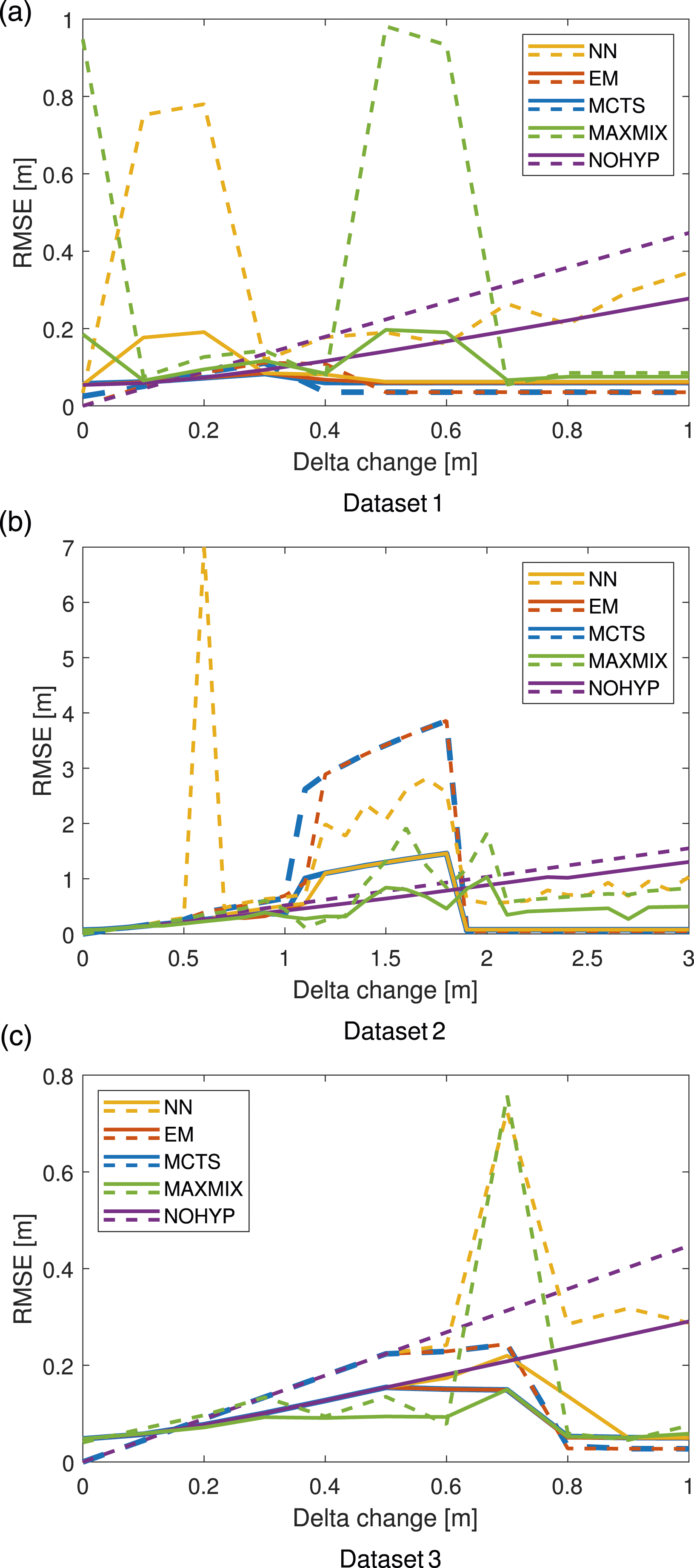

Results from dataset 1 and 3 show how the RMSE first increases when the landmarks are moved a short distance to then improve when the distance is large enough for hypotheses to be created. It is also visible that the selectors gives more similar results in estimating the robot position while MCTS and EM outperforms NN and max-mixture in estimating landmark positions. This suggests that all selectors are fairly good in selecting the correct mode when a landmark is in FOV, but the Markov property utilized in MCTS and EM adds value in retaining a good landmark position estimate. Both dataset 1 and dataset 3 are run with the same values of all tuning parameters, still, in dataset 1 the benefits of the multi-hypothesis approach can be seen already at landmark movements of 0.3 m while for dataset 3 it takes almost 0.9 m change before it takes full effect. This difference can be explained by how the gating depends on the currently estimated uncertainties. The confidence threshold for gating could be lowered to earlier create hypotheses also for dataset 3. This however, comes with the risk of creating lots of hypotheses caused by measurement noise that will degrade the computational speed. It is hard to quantify the delta change needed for hypothesis to be created in terms of uncertainty inputs to the system, since the environment setup and trajectory plays a big role here. Depending on how observations of non-moved landmarks have already been used and the shape of the already traveled trajectory, the current uncertainties can vary a lot causing observations from moved landmarks to be gated or not.

In dataset 2 the RMSE for the component selection methods is larger than for the NOHYP and max-mixture method just before the delta change is large enough to be fully discovered. This is an effect of the tuning trade-off in the gating threshold. The small change in the landmarks alters the robot position estimate just enough for measurements with large noise realizations to erroneously create hypotheses. If the gating threshold is increased to match these observations with the existing landmark position, the delta change needed for truly moved landmarks to be discovered is also increased, as is the case for dataset 3.

Dataset 2 highlights an interesting property due to the large chunk of the trajectory where no landmark is in FOV, the part marked with red in Figure 8. To get the optimization to converge after this part of the trajectory, also with zero landmark movement, the process noise is increased to $Q = d_{t}^{2} {0.03}^{2} I$ . At the first observation after the red part of the trajectory, the uncertainty in the robot pose in combination with the measurement noise and uncertainty in landmark positions, causes bad separation between the modes. This is also occurring at the very end of the trajectory, when the moved landmarks enter FOV after a long period of being non-visible. This situation is similar to what is seen in the simulation in Section 8.1 when the measurement noise is large. Inline with the results from that simulation, MCTS and EM outperforms the other component selectors in this situation. Noticeable for this dataset is how max-mixture is better than both MCTS and EM in the interval [1,1.9] in delta change, just before the change is fully perceived.

8.2.4. EM vs. MCTS

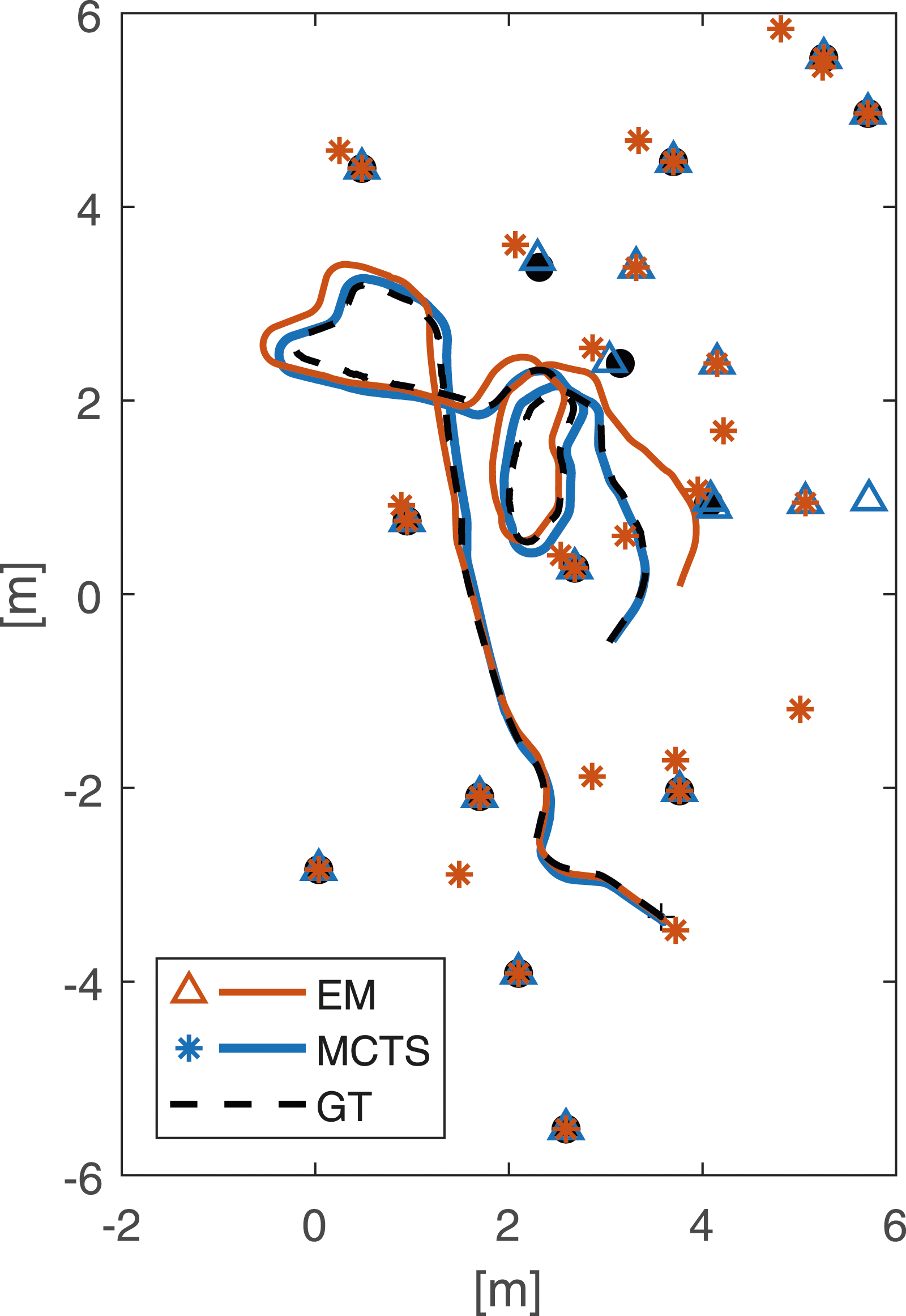
In the experiments presented in Figure 9 EM and MCTS as component selectors have very similar results. The difference between these two selectors is not visible until the selection becomes more complex. The two most important tuning parameters for the performance of the component selectors are the gating threshold α, and the probability of changing mode in the Markov model. There is a trade-off in creating too many unnecessary modes of landmarks that have not moved, and in potentially not creating modes of landmarks that have truly moved. This experiment is executed on dataset 1, with the transition probability significantly increased to 0.1 and the gating threshold lowered to α = 0.8 to create a lot more hypotheses. Results for MCTS and EM are seen in Figure 10. Now it is evident that MCTS copes with this situation a lot better. The EM method gets stuck in local minima for modes on landmarks that does not even move and therefore the result is very similar for all delta displacements. Also, when looking at the estimated positions in Figure 11, EM creates a lot more false modes.

Figure 10.

Resulting RMSE for dataset 1, when parameters are adjusted so that significantly more modes are created.

Figure 11.

Resulting trajectories for dataset 1, when parameters are adjusted so that significantly more modes are created. The orange stars marks all modes of all landmark created by the EM method, and the blue triangles marks all landmarks created by the MCTS method. These trajectories are created with a delta displacement of 1.0 m.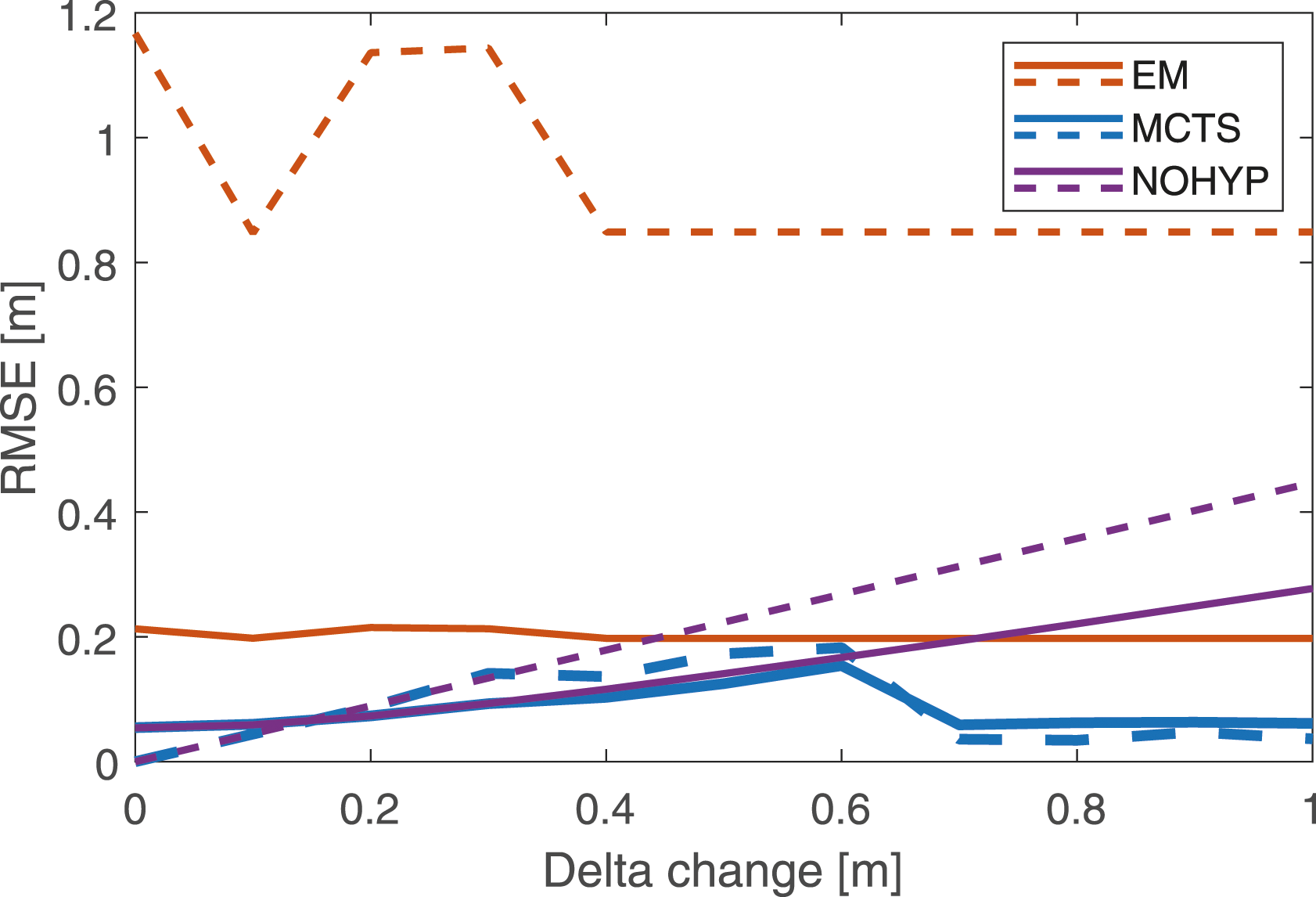

8.3. Computational cost

It is clear from the results presented in section 8.2 that MCTS is the most expressive and robust component selector. However, this comes with a computational cost, and in Table 1 it is seen that the average execution time is substantially longer for MCTS than for the other methods. These times should be considered in relation to the recording time of the datasets which are 340 s for all of them.

Table 1.

Average Execution Times for the experiments in section 8.2. The Times are given in Seconds and frames per second (FPS) for the Different Datasets (DS). The Right-most Columns are From the experiments in section 8.2.4 on Dataset 1 Where Significantly more Modes are Created.

	DS 1		DS 2		DS 3		more modes
	[s]	FPS	[s]	FPS	[s]	FPS	[s]	FPS
NN	27.8	35	50.4	16	26.3	40	–	–
EM	17.4	56	19.2	43	13.3	80	23.7	41
MCTS	303.6	13	608.8	1.3	122.1	8.7	2438	0.4
MAXMIX	16.5	59	21.0	39	21.5	49	–	–
NOHYP	8.2	119	13.4	61	12.7	84	–	–

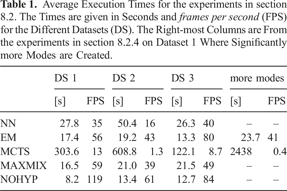
Worth noting in this comparison is that no specific effort has been put into optimizing the code since the focus of this experiment is on validation of the capabilities of the proposed methods. Although there are implementation aspects that could be considered. For example, a sliding window can be introduced in the mode selection phase. Executing with a sliding window of 40 s will reduce the average execution time of MCTS on dataset 2 from 608.8 s to 124.3 s, without any major loss in accuracy. Of course, reducing the size of the sliding window will eventually impact the accuracy and this trade-off has to be considered in accordance with the specific dataset and application requirements. To further optimize for speed, the roll-outs in the MCTS algorithm could be executed in parallel, which is not done in the current implementation. For all methods, the lion’s share of the execution time is for the small delta displacements. When a landmark movement is clearly detected, the re-linearization only executes once, and hence does not add much computational cost.

9. Conclusions

When aiming for long-term autonomy of mobile robots, changes in the environment are inevitable. Changes might cause erroneous data associations or false loop-closures that can have severe negative effects on the performance of a localization system. This paper have presented a system where a multi-hypothesis feature based map representation, capable of modeling discrete changes in landmark positions, is incorporated into a graph-based SLAM formulation to allow for continuous map updates during operation. A selector-mixture distribution have been proposed where a single component of a Gaussian mixture is selected for each time step, according to a selection criterion. By modeling the hypotheses of possible landmark positions as components in such a selector-mixture distribution, the simplicity of optimizing over a single Gaussian is preserved.

The selection criterion, given by the factor representation of the SLAM problem, consists of selecting a discrete mode of a landmark position in each time instance. This results in a factor graph with mixed discrete and continuous variables. An iterative optimization procedure have been suggested where the discrete variables are first estimated with the MCTS algorithm followed by a nonlinear least squares optimization on the continuous ones. Using MCTS for hypothesis selection reduces the risk of getting stuck in a local minimum. Experiments on both simulated and real data have shown that a non-static environment can successfully be navigated with the proposed method.

For these kinds of SLAM systems, real time execution is desirable. More effort needs to be put into optimizing and investigating the computational scalability. Also, the experiments in this paper utilize the assumption that all landmarks are uniquely identifiable. To increase applicability, it will be further investigated how the presented methods can be extended to allow for uncertainty in the landmark identities.

Footnotes

Declaration of conflicting interests

The author(s) declared no potential conflicts of interest with respect to the research, authorship, and/or publication of this article.

Funding

The author(s) disclosed receipt of the following financial support for the research, authorship, and/or publication of this article: This work was partially supported by the Wallenberg AI, Autonomous Systems and Software Program (WASP) funded by the Knut and Alice Wallenberg Foundation.

ORCID iD

Kristin Nielsen

References

Abdi

Ristaniemi

(2020) The max-product algorithm viewed as linear data-fusion. A distributed detection scenario 19(11): 7585–7597. DOI: 10.1109/twc.2020.3012910.

Agarwal

Mierle

The Ceres Solver Team (2022) Ceres solver. URL https://github.com/ceres-solver/ceres-solver.

Artan

Marshall

Lavigne

(2011) Robotic mapping of underground mine passageways. Mining Technology 120(1): 18–24. DOI: 10.1179/1743286311Y.0000000001.

Bar-Shalom

Willet

Tian

(2011) Tracking and Data Fusion: A Handbook of Algorithms. Bradford: YBS Publishing. ISBN 9780964831278.

Berrio

Ward

Worrall

, et al. (2019a) Identifying robust landmarks in feature-based maps. In: Proceedings of IEEE intelligent vehicles symposium (IV), Paris, France, 09–12 June 2019, pp. 1166–1172. DOI: 10.1109/IVS.2019.8814289.

Berrio

Ward

Worrall

, et al. (2019b) Updating the visibility of a feature-based map for long-term maintenance. In: Proceedings of IEEE intelligent vehicles symposium (IV), Paris, France, 09–12 June 2019, pp. 1173–1179. DOI: 10.1109/IVS.2019.8814189.

Bishop

(2006) Pattern Recognition and Machine Learning. Berlin: Springer Science.

Boström-Rost

Axehill

Hendeby

(2021) Sensor management for search and track using the poisson multi-bernoulli mixture filter. IEEE Transactions on Aerospace and Electronic Systems 57(5): 2771–2783. DOI: 10.1109/taes.2021.3061802.

Bresson

Alsayed

, et al. (2017) Simultaneous localization and mapping. A survey of current trends in autonomous driving 2(3): 194–220. DOI: 10.1109/tiv.2017.2749181.

10.

Browne

Powley

Whitehouse

, et al. (2012) A survey of Monte Carlo tree search methods. IEEE Transactions on Computational Intelligence and AI in Games 4(1): 1–43. DOI: 10.1109/tciaig.2012.2186810.

11.

Cadena

Carlone

Carrillo

, et al. (2016) Past, present, and future of simultaneous localization and mapping. Toward the robust-perception age 32(6): 1309–1332. DOI: 10.1109/TRO.2016.2624754.

12.

Chaslot

GMJB

Winands

MHM

van den Herik

(2008) Parallel monte-carlo tree search. In: Computers and Games. Berlin: Springer, pp. 60–71. DOI: 10.1007/978-3-540-87608-3_6.

13.

Chong

(2012) Graph approaches for data association. In: Proceedings of 15th international conference on information fusion, Singapore, 09–12 July 2012, pp. 1578–1585.

14.

Dai

Zhang

Zheng

, et al. (2021) RGB-D SLAM with moving object tracking in dynamic environments. IET Cyber-Systems and Robotics 3(4): 281–291. DOI: 10.1049/csy2.12019.

15.

Dellaert

GTSAM Contributors (2022) borglab/gtsam. URL. https://doi.org/10.5281/zenodo.5794541.

16.

Dellaert

Kaess

(2017) Factor graphs for robot perception. Foundations and Trends in Robotics 6(1–2): 1–139. DOI: 10.1561/2300000043.

17.

Doherty

Singh

, et al. (2022). Discrete-continuous smoothing and mapping. IEEE Robotics and Automation Letters 7(4): 12395–12402. DOI: 10.1109/LRA.2022.3216938.

18.

Hahnel

Triebel

Burgard

, et al. (2003) Map building with mobile robots in dynamic environments. In: Proceedings of IEEE international conference on robotics and automation (ICRA), Taipei, Taiwan, 14–19 September 2003, pp. 1557–1563. DOI: 10.1109/ROBOT.2003.1241816.

19.

Hsiao

Kaess

(2019) MH-iSAM2: multi-hypothesis iSAM using Bayes tree and hypo-tree. In: Proceedings of IEEE international conference on robotics and automation (ICRA), Montreal, QC, Canada, 20–24 May 2019, pp. 1274–1280. DOI:10.1109/ICRA.2019.8793854.

20.

Kaess

Dellaert

(2009) Covariance recovery from a square root information matrix for data association. Robotics and Autonomous Systems 57(12): 1198–1210. DOI: 10.1016/j.robot.2009.06.008.

21.

Kaess

Johannsson

Roberts

, et al. (2012) iSAM2: incremental smoothing and mapping using the Bayes tree. The International Journal of Robotics Research 31(2): 216–235. DOI: 10.1177/0278364911430419.

22.

Kocsis

Szepesvári

(2006) Bandit based Monte-Carlo planning. In: Proceedings of European Conference on Machine Learning. Berlin Heidelberg: Springer, pp. 282–293. DOI:10.1007/11871842_29.

23.

Kümmerle

Grisetti

Strasdat

, et al. (2011) G2o: a general framework for graph optimization. In: Proceedings of IEEE international conference on robotics and automation (ICRA), Shanghai, China, 09–13 May 2011, pp. 3607–3613. DOI: 10.1109/ICRA.2011.5979949.

24.

Latif

Cadena

Neira

(2013) Robust loop closing over time for pose graph SLAM. The International Journal of Robotics Research 32(14): 1611–1626. DOI: 10.1177/0278364913498910.

25.

Leung

KYK

Halpern

Barfoot

, et al. (2011) The UTIAS multi-robot cooperative localization and mapping dataset. The International Journal of Robotics Research 30(8): 969–974. DOI: 10.1177/0278364911398404.

26.

Hanebeck

(2021) Towards high-performance solid-state-LiDAR-inertial odometry and mapping. IEEE Robotics and Automation Letters 6(3): 5167–5174. DOI: 10.1109/LRA.2021.3070251.

27.

Huang

Doherty

, et al. (2021) Consensus-informed optimization over mixtures for ambiguity-aware object SLAM. In: Proceedings of IEEE/RSJ international conference on intelligent robots and systems (IROS), 27 September 2021 - 01 October 2021, Prague Czech Republic, pp. 5432–5439: IEEE. DOI: 10.1109/iros51168.2021.9636213.

28.

Montemerlo

Thrun

Koller

, et al. (2003) FastSLAM 2.0: an improved particle filtering algorithm for simultaneous localization and mapping that provably converges. In: Proceedings of the 18th international joint conference on artificial intelligence, Acapulco, Mexico, August 2003, pp. 1151–1156.

29.

Neal

Hinton

(1998) A View of the EM Algorithm that Justifies Incremental, Sparse, and Other Variants. Dordrecht: Springer Netherlands, pp. 355–368. DOI: 10.1007/978-94-011-5014-9_12.

30.

Neira

Tardos

(2001) Data association in stochastic mapping using the joint compatibility test 17(6): 890–897. DOI:10.1109/70.976019.

31.

Nielsen

Hendeby

(2022a) Feature based multi-hypothesis map representation for localization in non-static environments. In: Proceedings of 25th IEEE international conference on information fusion (FUSION), Linköping, Sweden, 04–07 July 2022, pp. 1–8. DOI: 10.23919/FUSION49751.2022.9841255.

32.

Nielsen

Hendeby

(2022b) Multi-hypothesis SLAM for non-static environments with reoccurring landmarks. IEEE Transactions on Intelligent Vehicles 8(4): 1–13. DOI: 10.1109/tiv.2022.3214978.

33.

Nobre

Heckman

Ozog

, et al. (2018) Online probabilistic change detection in feature-based maps. In: Proceedings of IEEE international conference on robotics and automation (ICRA), Brisbane, Australia, 21–25 May 2018, pp. 3661–3668: IEEE. DOI: 10.1109/icra.2018.8461111.

34.

Olson

Agarwal

(2013) Inference on networks of mixtures for robust robot mapping. The International Journal of Robotics Research 32(7): 826–840. DOI: 10.1177/0278364913479413.

35.

Pfeifer

Protzel

(2019) Expectation-maximization for adaptive mixture models in graph optimization. In: Proceedings of IEEE international conference on robotics and automation (ICRA), Montreal, QC, Canada, 20–24 May 2019, pp. 3151–3157: IEEE. DOI:10.1109/ICRA.2019.8793601.

36.

Pfingsthorn

Birk

(2013) Simultaneous localization and mapping with multimodal probability distributions. The International Journal of Robotics Research 32(2): 143–171. DOI: 10.1177/0278364912461540.

37.

Pitschl

Pryor

(2019) Obstacle persistent adaptive map maintenance for autonomous mobile robots using spatio-temporal reasoning. In: Proceedings of IEEE 15th international conference on automation science and engineering (CASE), Vancouver, Canada, 22–26 August 2019, pp. 1023–1028. DOI: 10.1109/COASE.2019.8843095.

38.

Rosen

Mason

Leonard

(2016) Towards lifelong feature-based mapping in semi-static environments. In: Proceedings of IEEE international conference on robotics and automation (ICRA), Stockholm, Sweden, 16–21 May 2016, pp. 1063–1070. DOI: 10.1109/icra.2016.7487237.

39.

Schadd

MPD

Winands

MHM

van den Herik

, et al. (2008) Single-player Monte-Carlo tree search. In: Computers and Games. Berlin: Springer, 1–12. DOI: 10.1007/978-3-540-87608-3_1.

40.

Schrittwieser

Antonoglou

Hubert

, et al. (2020) Mastering atari, go, chess and shogi by planning with a learned model. Nature 588(7839): 604–609. DOI: 10.1038/s41586-020-03051-4.

41.

Segal

Reid

(2014) Hybrid inference optimization for robust pose graph estimation. In: Proceedings of IEEE/RSJ international conference on intelligent robots and systems (IROS), Chicago, IL, USA, 142675–182682 September 2014. DOI: 10.1109/IROS.2014.6942928.

42.

Silver

Huang

Maddison

, et al. (2016) Mastering the game of Go with deep neural networks and tree search. Nature 529(7587): 484–489. DOI: 10.1038/nature16961.

43.

Strandmark

(2020) URL https://github.com/PetterS/monte-carlo-tree-search (accessed December 2022).

44.

Sünderhauf

Protzel

(2012a) Switchable constraints for robust pose graph SLAM. In: Proceedings of IEEE/RSJ international conference on intelligent robots and systems (IROS), Vilamoura-Algarve, Portugal, 07–12 October 2012, pp. 1879–1884. DOI: 10.1109/IROS.2012.6385590.

45.

Sünderhauf

Protzel

(2012b) Towards a robust back-end for pose graph SLAM. In: Proceedings of IEEE international conference on robotics and automation (ICRA), Saint Paul, MN, USA, 14–18 May 2012, pp. 1254–1261: IEEE. DOI: 10.1109/icra.2012.6224709.

46.

Wang

Thorpe

Thrun

(2003) Online simultaneous localization and mapping with detection and tracking of moving objects: theory and results from a ground vehicle in crowded urban areas. In: Proceedings of IEEE international conference on robotics and automation (ICRA), Taipei, Taiwan, 14–19 September 2003, 1, pp. 842–849. DOI: 10.1109/ROBOT.2003.1241698.

47.

Wang

Thorpe

Thrun

, et al. (2007) Simultaneous localization, mapping and moving object tracking. The International Journal of Robotics Research 26(9): 889–916. DOI: 10.1177/0278364907081229.

Hypothesis selection with Monte Carlo tree search for feature-based simultaneous localization and mapping in non-static environments

Abstract

Keywords

1. Introduction

2. Related work

3. Feature based SLAM with non-static landmarks

3.1. Multi-hypothesis map representation

3.2. Hypothesis Markov model

3.3. Multi-hypothesis SLAM

3.4. Hypotheses in a factor graph

4. Selector-mixture distribution

5. SLAM with component selector

5.1. Mixture SLAM

5.2. NN as component selector

5.3. EM as component selector

5.4. MCTS as component selector

6. Non-perfect sensors and negative information

6.1. Probability of detection

6.2. Negative information as a factor

7. Implementation aspects

7.1. Gating and mode creation

7.2. Negative information and probability of detection

8. Experiments and results

8.1. Simulated selector comparison

8.2. Real data experiment

8.2.1. The dataset

8.2.2. Parameter settings

8.2.3. Results

8.2.4. EM vs. MCTS

8.3. Computational cost

9. Conclusions

Footnotes

Declaration of conflicting interests

Funding

ORCID iD

References